OptORAMa: Optimal Oblivious RAM

(1)

OptORAMa: Optimal Oblivious RAM

∗

Gilad Asharov Bar-Ilan University

Ilan Komargodski NTT Research and Hebrew University of Jerusalem

Wei-Kai Lin Cornell University

Kartik Nayak

VMware and Duke University

Enoch Peserico Univ. Padova

Elaine Shi Cornell University

August 19, 2020

Abstract

Oblivious RAM (ORAM), first introduced in the ground-breaking work of Goldreich and Ostrovsky (STOC ’87 and J. ACM ’96) is a technique for provably obfuscating programs’ access patterns, such that the access patterns leak no information about the programs’ secret inputs. To compile a general program to an oblivious counterpart, it is well-known that Ω(logN) amortized blowup is necessary, whereN is the size of the logical memory. This was shown in Goldreich and Ostrovksy’s original ORAM work for statistical security and in a somewhat restricted model (the so called balls-and-bins model), and recently by Larsen and Nielsen (CRYPTO ’18) for computational security.

A long standing open question is whether there exists an optimalORAM construction that matches the aforementioned logarithmic lower bounds (without making large memory word assumptions, and assuming a constant number of CPU registers). In this paper, we resolve this problem and present the first secure ORAM with O(logN) amortized blowup, assuming one-way functions. Our result is inspired by and non-trivially improves on the recent beautiful work of Patel et al. (FOCS ’18) who gave a construction with O(logN ·log logN) amortized blowup, assuming one-way functions.

One of our building blocks of independent interest is a linear-time deterministic oblivious algorithm for tight compaction: Given an array ofnelements where some elements are marked, we permute the elements in the array so that all marked elements end up in the front of the array. Our O(n) algorithm improves the previously best known deterministic or randomized algorithms whose running time isO(n·logn) orO(n·log logn), respectively.

Keywords: Oblivious RAM, randomized algorithms, compaction.

∗

Errata: The scheme in this version is almost identical to the version posted on Cryptology eprint on Dec 11, 2018. The only slight difference is that when we rebuild levels 1,2, . . . , j−1 into the next empty levelj, we empty only the elements in the oblivious dictionaryD marked with levelsj−1 or smaller. We do not empty elements in

(2)

1 Introduction

Oblivious RAM (ORAM), first proposed by Goldreich and Ostrovsky [29,31], is a technique to compile any program into a functionally equivalent one, but whose memory access patterns are independent of the program’s secret inputs. The overhead of an ORAM is defined as the (multiplicative) blowup in runtime of the compiled program. Since Goldreich and Ostrovsky’s seminal work, ORAM has received much attention due to its applications in cloud computing, secure processor design, multi-party computation, and theoretical cryptography (for example, [6,25,26,28,45–47,51,57,59,60,64,67,68])

For more than three decades, the biggest open question in this line of work is regarding the

optimaloverhead of ORAM. Goldreich and Ostrovsky’s original work [29,31] showed a construction withO(log3N) blowup in runtime, assuming the existence of one-way functions, where N denotes the memory size consumed by the original non-oblivious program. On the other hand, they proved that any ORAM scheme must incur at least Ω(logN) overhead, but their lower bound is restricted to schemes that treat the contents of each memory word as “indivisible” (see Boyle and Naor [7]) and make no cryptographic assumptions. In a recent work, Larsen and Nielsen [41] showed that Ω(logN) overhead is necessary for allonline ORAM schemes,1even ones that use cryptographic assumptions and might perform non-trivial encodings on the contents of the memory. Since Goldreich and Ostrovsky’s work, a long line of research has been dedicated to improving the asymptotic efficiency of ORAM [12,33,40,58,61,63]. Prior to our work, the best known scheme, allowing computational assumptions, is the elegant work by Patel et al. [53]: they showed the existence of an ORAM withO(logN·log logN) overhead, assuming one-way functions. In comparison with Goldreich and Ostrovksy’s originalO(log3N) result, Patel’s result seems tantalizingly close to matching the lower bound, but unfortunately we are still not there yet and the construction of an optimal ORAM continues to elude us even after more than 30 years.

1.1 Our Results: Optimal Oblivious RAM

We resolve this long-standing problem by showing a matching upper bound to Larsen and Nielsen’s [41] lower bound: an ORAM scheme withO(logN) overhead and negligible security inλ, whereN is the size of the memory and λis the security parameter, assuming one-way functions. More concretely, we show: 2

Theorem 1.1. Assume that there is a PRF family that is secure against any probabilistic polynomial-time adversary except with a negligible small probability inλ. Assume thatλ≤N ≤T ≤poly(λ)for any fixed polynomial poly(·), whereT is the number of accesses. Then, there is an ORAM scheme with O(logN) overhead and whose security failure probability is upper bounded by a suitable negligible function inλ.

In the aforementioned results and throughout this paper, unless otherwise noted, we shall assume a standard word-RAM where each memory word has at least w = logN bits, i.e., large enough to store its own logical address. We assume that word-level addition and boolean operations can be done in unit cost. We assume that the CPU has constant number of private registers. For our ORAM construction, we additionally assume that a single evaluation of a pseudorandom function

1_{An ORAM scheme is}_online_{if it supports accesses arriving in an online manner, one by one. Almost all known}

schemes have this property.

(4)

(PRF), resulting in at least word-size number of pseudo-random bits, can be done in unit cost.3 Note that all earlier computationally secure ORAM schemes, starting with the work of Goldreich and Ostrovsky [29,31], make the same set of assumptions. Additionally, we remark that our result can be made statistically secure if one assumes a private random oracle to replace the PRF (the known logarithmic ORAM lower bound [29,31,41] still hold in this setting). Finally, we note that our construction suffers from huge constants due to the use of certain expander graphs; improving the concrete constant is left for future work.

In Appendix A we provide a comparison with previous works, where we make the comparison more accurate and meaningful by explicitly stating the dependence on the error probability (which was assumed to be some negligible functions in previous works).

1.2 Our Results: Optimal Oblivious Tight Compaction

Closing the remaining log logN gap for ORAM turns out to be highly challenging. Along the way, we actually construct an important building block, that is, a deterministic, linear-time, oblivious

tight compactionalgorithm. This result is an important contribution on its own, and has intimate connections to classical algorithms questions, as we explain below.

Tight compaction is the following task: given an input array of size n containing either real or dummy elements, output a permutation of the input array where all real elements appear in the front. Tight compaction can be considered as a restricted form of sorting, where each element in the input array receives a 1-bit key, indicating whether it is real or dummy. One na¨ıve solution for tight compaction, therefore, is to rely on oblivious sorting to sort the input array [1,32]; unfortunately, due to recent lower bounds [22,44], we know that any oblivious sorting scheme must incur Ω(n·logn) time on a word-RAM, either assuming that the algorithm treats each element as “indivisible” [44] or assuming that the famous Li-Li network coding conjecture [43] is true [22].

A natural question, therefore, is whether we can do asymptotically better than just na¨ıvely sorting the input. It turns out that this question is related to a line of work in the classical algorithms literature, that is, the design of switching networks and routing on such networks [1,4,5,23,55,56]. First, a line of combinatorial works showed the existence of linear-sized super-concentrators [54,55,

62], i.e., switching networks withninputs andnoutputs such that vertex-disjoint paths exist from any k elements in the inputs to any k positions in the outputs. One could leverage a linear-sized super-concentrator construction toobliviouslyroute all the real elements in the input to the front of the output array deterministically and in linear time (by routing elements along the routes), but it is not clear yet how to find routes (i.e., a set of vertex-disjoint paths) from the real input positions to the front of the output array.

In an elegant work in 1996, Pippenger [56] showed a deterministic, linear-time algorithm for route-finding but unfortunately the algorithm is not oblivious. Shortly afterwards, Leighton et al. [42] showed a probabilistic algorithm that tightly compacts n elements in O(n·log logλ) time with 1−negl(λ) probability — their algorithm isalmost oblivious except for leaking the number of reals and dummies. After Leighton et al. [42], this line of work remained somewhat stagnant for almost two decades. Only recently, did we see some new results: Mitchell and Zimmerman [49] as well as Lin et al. [44] showed how to achieve the same asymptotics as Leighton et al. [42] but now making the algorithm fully oblivious.

In this paper, we give an explicit construction of a deterministic, oblivious algorithm that tightly compacts any input array of nelements in linear time, as stated in the following theorem:

3

(5)

Theorem 1.2 (Linear-time oblivious tight compaction). There is a deterministic, oblivious tight compaction algorithm that compacts nelements in O(dD/we ·n) time on a word-RAM where Dis the bit-width for encoding each element and w≥logn is the word size.

Our algorithm is not comparison-based and not stable and this is inherent. Specifically, Lin et al. [44] recently showed that any stable, oblivious tight compaction algorithm (that treats elements as indivisible) must incur Ω(n·logn) runtime, where stability requires that the real elements in the output must appear in the same order as the input. Further, due to the well-known 0-1 principle [18,66], any comparison-based tight compaction algorithm must incur at least Ω(n·logn) runtime as well.4

Not only our ORAM construction relies on the above compaction algorithm in several key points, but it is a useful primitive independently. For example, we use our compaction algorithm to give a perfectly oblivious algorithm that randomly permutes arrays ofnelements in (worst-case)

O(n·logn) time. All previously known such constructions have some probability of failure.

2 Technical Roadmap

We give a high-level overview of our results. In Section2.1we provide a high-level overview of our ORAM construction which uses an oblivious tight compaction algorithm. In Section 2.2we give a high-level overview of the techniques underlying our tight compaction algorithm.

2.1 Oblivious RAM

In this section we present a high-level description of the main ideas and techniques underlying our ORAM construction. Full details are given later in the corresponding technical sections.

Hierarchical ORAM. The hierarchical ORAM framework, introduced by Goldreich and Ostro-vsky [29,31] and improved in subsequent works (e.g., [12,33,40]), works as follows. For a logical memory ofN blocks, we construct a hierarchy of hash tables, henceforth denotedT1, . . . , TLwhere

L = logN. Each Ti stores 2i memory blocks. We refer to tableTi as the i-th level. In addition,

we store next to each table a flag indicating whether the table isfull orempty. When receiving an access request toread/writesome logical memory address addr, the ORAM proceeds as follows:

• Read phase. Access each non-empty levelsT1, . . . , TLin order and performLookupforaddr.

If the item is found in some level Ti, then when accessing all non-empty levels Ti+1, . . . , TL

look for dummy.

• Write back. If this operation isread, then store the found data in the read phase and write back the data value toT0. If this operation is write, then ignore the associated data found in the read phase and write the value provided in the access instruction inT0.

• Rebuild: Find the first empty level`. If no such level exists, set`:=L. Merge all{Tj}0≤j≤`

intoT`. Mark all levels T1, . . . , T`−1 as empty and T` as full.

For each access, we perform logN lookups, one per hash table. Moreover, after t accesses, we rebuild the i-th table dt/2ie times. When implementing the hash table using the best known oblivious hash table (e.g., oblivious Cuckoo hashing [12,33,40]), building a level with 2k items obliviously requiresO(2k·log(2k)) =O(2k·k) time. This building algorithm is based on oblivious

4

(6)

sorting, and its time overhead is inherited from the time overhead of the oblivious sort procedure (specifically, the best known algorithm for obliviously sorting nelements takesO(n·logn) time [1,

32]). Thus, summing over all levels (and ignoring the logN lookup operations across different levels for each access), t accesses requirePlogN

i=1

_t

2i

·O(2i·i) =O(t·log2N) time. On the other hand, lookup takes essentially constant time per level (ignoring searching in stashes which introduce an additive factor) and thisO(logN) per access. Thus, there is an asymmetry between build time and lookup time, and the main overhead is the build.

The work of Patel et al. [53]. Classically (e.g., [12,29,31,33,40]), oblivious hash tables were built to support (and be secure for) every input array. This required expensive oblivious sorting, causing the extra logarithmic factor. The key idea of Patel et al. [53] is to modify the hierarchical ORAM framework to realize ORAM from a weaker primitive: an oblivious hash table that works only forrandomly shuffled inputarrays. Patel et al. describe a novel oblivious hash table such that building a hash table containing n elements can be accomplished without oblivious sorting and consumes onlyO(n·log logλ) total time5 and lookup consumesO(log logn) total time. Patel et al. argue that their hash table construction retains security not necessarily for every input, but when the input array is randomly permuted, and moreover the input permutation must be unknown to the adversary.

To be able to leverage this relaxed hash table in hierarchical ORAM, a remaining question is the following: whenever a level is being rebuilt in the ORAM (i.e., a new hash table is being constructed), how do we make sure that the input array is randomly and secretly shuffled? A na¨ıve answer is to employ an oblivious random permutation to permute the input, but known oblivious random permutation constructions require oblivious sorting which brings us back to our starting point. Patel et al. solve this problem and show that there is no need to completely shuffle the input array. Recall that when building some level T`, the input array consists of only unvisited

elements in tables T0, . . . , T`−1 (and T` too if ` is the largest level). Patel et al. argue that the

unvisited elements in tablesT0, . . . , T`−1 are already randomly permutedwithin each table and the permutation is unknown to the adversary. Then, they presented a new algorithm, called multi-array shuffle, that combines these arrays to a shuffled array within O(n·log logλ) time, where

n = |T0|+|T1|+ . . .+|T`−1|.6 The algorithm is somewhat involved, randomized, and has a negligible probability of failure.

The blueprint. Our construction builds upon and simplifies the construction of Patel et al. To get better asymptotic overhead, we improve their construction in two different aspects:

1. We show how to implement our variant of multi-array shuffle (called intersperse) in O(n) time. Specifically, we show a new reduction fromintersperse to tight compaction.

2. We develop a hash table that supports build in O(n) time assuming that the input array is randomly shuffled. The lookup is O(1), ignoring time spent on looking in stashes. Achieving this is rather non-trivial: first we use a “packing” style trick to construct oblivious Cuckoo hash tables for small sizes where n≤polylogλ, achieving linear-time build and constant-time lookup. Relying on the advantage we gain for problems of small sizes, we then show how to solve problems of medium and large sizes, again relying on oblivious tight compaction as a building

5

λdenotes the security parameter. Since the size of the hash tablenmay be small, here we separate the security parameter from the hash table’s size.

6_{The time overhead is a bit more complicated to state and the above expression is for the case where}_|_T

(7)

block. The bootstrapping step from medium to large is inspired by Patel et al. [53] at a very high level, but our concrete construction differs from Patel et al. [53] in many technical details.

We describe the core ideas behind these improvements next. In Section 2.1.1, we present our multi-array shuffle algorithm. In Section2.1.2, we show how to construct a hash table for shuffled inputs achieving linear build time and constant lookup.

2.1.1 Interspersing Randomly Shuffled Arrays

Given two arrays,I1 andI2, of sizen1, n2, respectively, where each array is randomly shuffled, our goal is to output a single array that contains all elements from I1 and I2 in a randomly shuffled order. Ignoring obliviousness, we could first initialize an output array of size n =n1+n2, mark exactly n1 random locations in the output array, and place the elements from I1 arbitrarily in these locations. The elements fromI2 are placed in the unmarked locations.7 The challenge is how to perform this placement obliviously, without revealing the mapping from the input array to the output array.

We observe that this routing problem is exactly the “reverse” problem of oblivious tight com-paction, where one is given an input array of sizencontaining keys that are 1-bit and the goal is to sort the array such that all elements with key 0 appear before all elements with key 1. Intuitively, by running this algorithm “in reverse”, we obtain a linear time algorithm for obliviously routing marked elements to an array with marked positions (that are not necessarily at the front). Since we believe that this procedure is useful in its own right, we formalize it independently and call it

oblivious distribution. The full details appear in Section 6.

2.1.2 An Optimal Hash Table for Shuffled Inputs

In this section, we first describe a warmup construction that can be used to build a hash table in

O(n·polylog logλ) time and supports lookups inO(polylog logλ) time. We will then get rid of the additionalpolylog logλfactor in both the build and lookup phases.

Warmup: oblivious hash table with polylog logλ slack. Intuitively, to build a hash table, the idea is to randomly distribute the n elements in the input into B := n/polylogλ bins of size polylogλ in the clear. The distribution is done according to a pseudorandom function with some secret key K, where an element with address addr is placed in the bin with index PRFK(addr).

Whenever we lookup for a real element addr0, we access the bin PRFK(addr0); in which case, we

might either find the element there (if it was originally one of the n elements in the input) or we might not find it in the accessed bin (in the case where the element is not part of the input array). Whenever we perform a dummy lookup, we just access a random bin.

Since we assume that thenballs are secretly and randomly distributed to begin with, the build procedure does not reveal the mapping from original elements to bins. However, a problem arises in the lookup phase. Since the total number of elements in each bin is revealed, accessing in the lookup phase all real keys of the input array would produce an access pattern that is identical to that of the build process, whereas accessing n dummy elements results in a new, independent balls-into-bins process of nballs into B bins.

To this end, we first throw the n balls into the B bins as before, revealing loads n1, . . . , nB.

Then, we sample newsecret loadsL1, . . . , LBcorresponding to an independent process of throwing

7

Note that the number of such assignments is _nn 1,n2

. Assuming that each array is already permuted, the number of possible outputs is _nn

1,n2

(8)

n0 := n·(1−1/polylogλ) balls into B bins. By a Chernoff bound, with overwhelming probability

Li < ni for every i ∈ [B]. We extract from each bin arbitrary ni −Li elements obliviously

and move them to an overflow pile (without revealing the Li’s). The overflow pile contains only

n/polylogλ elements so we use a standard Cuckoo hashing scheme such that it can be built in

O(m·logm) =O(n) time and supports lookups effectively inO(1) time (ignoring the stash).8 The crux of the security proof is showing that since the secret loadsL1, . . . , LB are never revealed, they

are large enough to mask the access pattern in the lookup phase so that it looks independent of the one leaked in the build phase.

We glossed over many technical details, the most important ones being how the bin sizes are truncated to the secret loads L1, . . . , LB, and how each bin is being implemented. For the second

question, since the bins are ofO(polylogλ) size, we support lookups using a perfectly secure ORAM constructions that can be built in O(polylogλ·polylog logλ) and looked up in O(polylog logλ) time [14,19] (this is essentially where ourpolylog log factor comes from in this warmup). The first question is slightly more tricky and here we employ our linear time tight compaction algorithm to extract the number of elements we want from each bin.

The full details of the construction appear in Section 7.

Remark 2.1 (Comparison of the warmup construction with Patel et al. [53]). Our warmup con-struction borrows the idea of revealing loads and then sampling new secret loads from Patel et al. However, our concrete instantiation is different and this difference is crucial for the next step where we get an optimal hash table. Particularly, the construction of Patel et al. has log logλ layers of hash tables of decreasing sizes, and one has to look for an element in each one of these hash tables, i.e., searching withinlog logλbins. In our solution, by tightening the analysis (that is, the Chernoff bound), we show that a single layer of hash tables suffices; thus, lookup accesses only a single bin. This allows us to focus on optimizing the implementation of a bin towards the optimal construction.

Oblivious hash table with linear build time and constant lookup time. In the warmup construction, (ignoring the lookup time in the stash of the overflow pile9), the only super-linear operation that we have is the use of a perfectly secure ORAM, which we employ for bins of size

O(polylogλ). In this step, we replace this with a data structure with linear time build and constant time lookup: a Cuckoo hash table for lists of polylogarithmic size.

Recall that in a Cuckoo hash table each element receives two random bin choices (e.g., deter-mined by a PRF) among a total ofccuckoo·n bins where ccuckoo>1 is a suitable constant. During build-time, the goal is for all elements to choose one of the two assigned bins, such that every bin receives at most one element. At this moment it is not clear how to accomplish this build process, but suppose we can obliviously build such a Cuckoo hash table in linear time, then the problem would be solved. Specifically, once we have built such a Cuckoo hash table, lookup can be accom-plished in constant time by examining both bin choices made by the element (ignoring the issue of the stash for now). Since the bin choices are (pseudo-)random, the lookup process retains security as long as each element is looked up at most once. At the end of the lookups, we can extract the unvisited elements through oblivious tight compaction in linear time — it is not hard to see that if the input array is randomly shuffled, the extracted unvisited elements appear in a random order too.

8

We refer to Section4.5for background information on Cuckoo hashing.

9_{For the time being, the reader need not worry about how to perform lookup in the stash. Later, when we use}

(9)

Therefore the crux is how to build the Cuckoo hash table for polylogarithmically-sized, randomly shuffled input arrays. Our observation is that classical oblivious Cuckoo hash table constructions can be split into three steps: (1) assigning two possible bin choices per element, (2) assigning either one of the bins or the stash for every element, and (3) routing the elements according to the Cuckoo assignment. We delicately handle each step separately:

1. For step (1) the n=polylogλelements in the input array can each evaluate the PRF on its associated key, and write down its two bin choices (this takes linear time).

2. Implementing step (2) in linear time is harder as this step is dominated by a sequence of oblivious sorts. To overcome this, we use the fact that the problem sizenis of sizepolylogλ. As a result, the index of each item and its two bin choices can be expressed usingO(log logλ)

bits which means that a single memory word (which is logλbits long) can hold O

logλ

log logλ

many elements’ metadata. We can now apply a “packed sorting” type of idea [2,13,17,36] where we use the RAM’s word-level instructions to perform SIMD-style operations. Through this packing trick, we show that oblivious sorting and oblivious random permutation (of the elements’ metadata) can be accomplished inO(n) time!

3. Step (3) is classically implemented using oblivious bin distribution which again uses oblivious sorts. Here, we cannot use the packing trick since we operate on the elements themselves, so we use the fact that the input array is randomly shuffled and just route the elements in the clear.

There are many technical issues we glossed over, especially related to the fact that the Cuckoo hash tables are of size ccuckoo·n bins, where ccuckoo >1. This requires us to pad the input array with dummies and later to use them to fill the empty slots in the Cuckoo assignment. Additionally, we also need to get rid of these dummies when extracting the set of unvisited element. All of these require several additional (packed) oblivious sorts or our oblivious tight compaction.

We refer the reader to Section 8 for the full details of the construction.

2.1.3 Additional Technicalities

The above description, of course, glossed over many technical details. To obtain our final ORAM construction, there are still a few concerns that have not been addressed. First, recall that we need to make sure that the unvisited elements in a hash table appear in a (pseudo-)random order such that we can make use of this residual randomness to re-initialize new hash tables faster. To guarantee this for the Cuckoo hash table that we employ forpolylogλ-sized bins, we need that the underlying Cuckoo hash scheme we employ satisfy an additional property called the “indiscrim-inating bin assignment” property: specifically, we need that the two pseudo-random Cuckoo-bin choices for each element do not depend on the order in which they are added, their keys, or their positions in the input array. In our technical sections later, this property will allow us to do a coupling argument and prove that the residual unvisited elements in the Cuckoo hash table appear in random order.

(10)

Kushilevitz et al. [40] to merge all stashes into a common stash of size O(log2λ), which is added to the smallest level when it is rebuilt.

On deamortization. As the overhead of our ORAM is amortized over several accesses, it is natural to ask whether we can deamortize the construction to achieve the same overhead in the worst case, per access. Historically, Ostrovsky and Shoup [51] deamortized the hierarchical ORAM of Goldreich and Ostrovsky [31], and related techniques were later applied on other hierarchical ORAM schemes [12,34,40]. Unfortunately, the technique fails for our ORAM as we explain below (it fails for Patel et al. [53], as well, by the same reason).

Recall that in the hierarchical ORAM, thei-th level hash table stores 2ikeys and is rebuilt every 2i accesses. The core idea of existing deamortization techniques is to spread the rebuilding work over the next sequence of 2i ORAM accesses. That is, copy the 2i keys (to be rebuilt) to another working space while performing lookup on the same levelito fulfill the next 2i accesses. However, plugging such copy-while-accessing into our ORAM, an adversary can access a key in level iright after the same level is fully copied (as the copying had no way to foresee future accesses). Then, in the adversarial eyes, the copied keys are no longer randomly shuffled, which breaks the security of the hash table (which assumes that the inputs are shuffled). Indeed, in previous works, where hash tables were secure for every input, such deamortization works. Deamortizing our construction is left as an open problem.

2.2 Tight Compaction

Recall that tight compaction can be considered as a restricted form of sorting, where each element in the input array receives a 1-bit key, indicating whether it is real or dummy. The goal is to move all the real elements in the array to the front obliviously, and without leaking how many elements are reals. We show a deterministic algorithm for this task.

Reduction to loose compaction. Pippenger’s self-routing super-concentrator construction [56] proposes a technique that reduces the task of tight compaction to that of loose compaction. Infor-mally speaking, loose compaction receives as input a sparse array, containing a few real elements and many dummy elements. The output is a compressed output array, containing all real elements but the procedure does not necessarily remove all the dummy elements. More concretely, we care about a specific form of loose compactor (parametrized by n): consider a suitable bipartite ex-pander graph that has n vertices on the left and n/2 vertices on the right where each node has constant degree. At most 1/128 fraction of the vertices on the left will receive a real element, and we would like to routeallreal elements over vertex-disjoint paths to the right side such that every right vertex receives at most 1 element. The crux is to find a set of satisfying routes in linear time and obliviously. Once a set of feasible routes have been identified, it is easy to see that performing the actual routing can be done obliviously in linear time (and for obliviousness we need to route a dummy element over an edge that bears 0 load). During this process, we effectively compress the sparse input array (represented by vertices on the left) by 1/2 without losing any element.

Using Pippenger’s techniques [56] and with a little extra work, we can derive the following claim — at this point we simply state the claim while deferring algorithmic details to subsequent technical sections. BelowDdenotes the number of bits it takes to encode an element andwdenotes the word size:

(11)

construct an oblivious algorithm that tightly compactsnelements in timeC·T(n)+C0·dD/we·n

for all n≤n0.

As mentioned, the crux is to find satisfying routes for such a “loose compactor” bipartite graph obliviously and in linear time. Achieving this is non-trivial: for example, the recent work of Chan et al. [14] attempted to do this but their route-finding algorithm requires O(nlogn) runtime — thus Chan et al. [14]’s work also implies a loose compaction algorithm that runs in timeO(nlogn+

dD/we·n). To remove the extra lognfactor, we introduce two new ideas,packing, anddecomposition

— in fact both ideas are remotely reminiscent of a line of works in the core algorithms literature on (non-comparison-based, non-oblivious) integer sorting on RAMs [2,17,36] but obviously we apply these techniques to a different context.

Packing: linear-time compaction for small instances. We observe that the offline route-finding phase operates only on metadata. Specifically, the route-route-finding phase receives the following as input: an array of nbits where the i-th bit indicates whether the i-th input position is real or dummy. If the problem size nis small, specifically, if n ≤w/logw where w denotes the width of a memory word, we can pack the entire problem into a single memory word (since each element’s index can be described in logn bits). In our technical sections we will show how to rely on word-level addition and boolean operations to solve such small problem instances in O(n) time. At a high level, we follow the slow route-finding algorithm by Chan et al. [14], but now within a single memory word, we can effectively perform SIMD-style operations and we exploit this to speed up Chan et al. [14]’s algorithm by a logarithmic factor for small instances.

Relying on the above Claim that allows us to go from loose to tight, we now have anO(n)-time oblivious tight compaction algorithm for small instances where n ≤ w/logw; specifically, if the loose compaction algorithm takes C0·ntime, then the runtime of the tight compaction would be upper bounded byC·C0·n+C0· dD/we ·n≤C·C0·C0· dD/we ·n.

Decomposition: bootstrapping larger instances of compaction. With this logarithmic advantage we gain in small instances, our hope is to bootstrap larger instances by decomposing larger instances into smaller ones.

Our bootstrapping is done in two steps — as we calculate below, each time we bootstrap, the constant hidden inside the O(n) runtime blows up by a constant factor; thus it is important that the bootstrapping is done for onlyO(1) times.

1. Medium instances: n ≤ (w/logw)2_. _{For medium instances, our idea is to divide the input} array into √n segments each of B := √n size. As long as the input array has only n/128 or fewer real elements, then at most √n/4 segments can be dense, i.e., each containing more than √n/4 real elements (1/4 is loose but sufficient). We rely on tight compaction for small segments to move the dense segments in front of the sparse ones. For each of the 3√n/4 segments, we next compress away 3/4 of the space for using tight compaction for small instances. Clearly, the above procedure is a loose compaction and consumes at most 2·C·C0·C0· dD/we ·n+ 6dD/we ·n≤2.5·C·C0·C0· dD/we ·nruntime.

So far we have constructed a loose compaction algorithm for medium instances. Using the aforementioned Claim, we can in turn construct an algorithm that obliviously and tightly

compacts a medium-sized instance of sizen≤(w/logw)2_{in time at most 3}_C2_·_C0_·_C

0·dD/we·n.

(12)

elements. Similar to the medium case, at most 1/4 fraction of the segments can have real density exceeding 1/4 — which we call such segmentsdense. As before, we would like to move the dense segments in the front and the sparse ones to the end. Recall that Chan et al. [14]’s algorithm solves loose compaction for problems of arbitrary size m in time C1 ·(mlogm+ dD/wem) Thus due to the above claim we can solve tight compaction for problems of any sizem in timeC·C1·(mlogm+dD/we ·m) +C0· dD/we ·m. Thus, inO(dD/we ·n) time we can move all the dense instances to the front and the sparse instances to the end. Finally, by invoking medium instances of tight compaction, we can compact within each segment in time that is linear in the size of the segment. This allows us to compress away 3/4 of the space from the last 3/4 segments which are guaranteed to be sparse. This gives us loose compaction for large instances inO(dD/we ·n) time — from here we can construct oblivious tight compaction for large instances using the above Claim.10

Remark 2.2. In our formal technical sections later, we in fact directly use loose compaction for smaller problem sizes to bootstrap loose compaction for larger problem sizes (whereas in the above version we use tight compaction for smaller problems to bootstrap loose compaction for larger problems). The detailed algorithm is similar to the one described above: it requires slightly more complicated parameter calculation but results in better constants than the above more intuitive ver-sion.

3 Preliminaries

Throughout this work, the security parameter is denoted λ, and it is given as input to algo-rithms in unary (i.e., as 1λ). A function negl:N → R+ is negligible if for every constant c > 0

there exists an integer Nc such that negl(λ) < λ−c for all λ > Nc. Two sequences of

ran-dom variables X = {Xλ}λ∈N and Y = {Yλ}λ∈N are computationally indistinguishable if for any probabilistic polynomial-time algorithm A, there exists a negligible function negl(·) such that

Pr[A(1λ, X_λ) = 1]−Pr[A(1λ, Y_λ) = 1]

≤ negl(λ) for all λ ∈ N. We say that X ≡ Y for such

two sequences if they define identical random variables for every λ ∈ N. The statistical

dis-tance between two random variables X and Y over a finite domain Ω is defined by SD(X, Y) , 1

2 ·

P

x∈Ω|Pr[X=x]−Pr[Y =x]|. For an integer n∈N we denote by [n] the set{1, . . . , n}. By k we denote the operation of string concatenation.

Definition 3.1 (Pseudorandom functions (PRFs)). Let PRF be an efficiently computable function family indexed by keys sk ∈ {0,1}λ_{, where each} _PRF

sk takes as input a value x ∈ {0,1}n(λ) and

outputs a value y ∈ {0,1}m(λ)_{. A function family} _PRF _is _δA_-secure _{if for every (non-uniform)}

probabilistic polynomial-time algorithm A, it holds that

Pr sk←{0,1}λ

h

APRFsk(·)₍₁λ_{) = 1}

i

− Pr

f←Fλ

h

Af(·)(1λ) = 1

i

≤δA(λ),

for all large enough λ∈_N, where Fλ is the set of all functions that map{0,1}n(λ) into {0,1}m(λ).

It is known that one-way functions are existentially equivalent to PRFs for any polynomialn(·) andm(·) and negligibleδA(·) [37,50]. Our construction will employ PRFs in several places and we present each part modularly with its own PRF, but note that the whole ORAM construction can be implemented with a single PRF from which we can implicitly derive all other PRFs.

10_{We omit the concrete parameter calculation in the last couple of steps but from the calculations so far, it should}

(13)

3.1 Oblivious Machines

We define oblivious simulation of (possibly randomized) functionalities. We provide a unified framework that enables us to adopt composition theorems from secure computation literature (see, for example, Canetti and Goldreich [9,10,30]), and to prove constructions in a modular fashion.

Random-access machines. A RAM is an interactive Turing machine that consists of a memory and a CPU. The memory is denoted as mem[N, w], and is indexed by the logical address space [N] = {1,2, . . . , N}. We refer to each memory word also as a block and we use w to denote the bit-length of each block. The CPU has an internal state that consists of O(1) words. The memory supports read/write instructions (op,addr,data), whereop∈ {read,write},addr∈[N] and data ∈ {0,1}w_{∪ {⊥}}_{. If} _op ₌ _read_{, then} _data ₌ _⊥ _{and the returned value is the content of the}

block located in logical addressaddr in the memory. Ifop=write, then the memory data in logical address addr is updated to data. We use standard setting thatw= Θ(logN) (so a word can store an address). We follow the convention that the CPU performs one word-level operation per unit time, i.e., arithmetic operations (addition or subtraction), bitwise operations (AND, OR, NOT, or shift), memory accesses (read or write), or evaluating a pseudorandom function [12,31,33,40,41,53].

Oblivious simulation of a (non-reactive) functionality. We consider machines that interact with the memory viaread/writeoperations. We are interested in defining sub-functionalities such as oblivious sorting, oblivious shuffling of memory contents, and more, and then define more complex primitives by composing the above. For simplicity, we assume for now that the adversary cannot see memory contents, and does not see thedatafield in each operation (op,addr,data) that the memory receives. That is, the adversary only observes (op,addr). One can extend the constructions for the case where the adversary can also observe data using symmetric encryption in a straightforward way.

We define oblivious simulation of a RAM program. Let f:{0,1}∗ → {0,1}∗ be a (possibly randomized) functionality in the RAM model. We denote the output off on inputxto bef(x) =y. Oblivious simulation of f is a RAM machine Mf that interacts with the memory, has the same

input/output behavior, but its access pattern to the memory can be simulated. More precisely, we let (out,Addrs) ← Mf(x) be a pair of random variable that corresponds to the output of Mf on

inputxand whereAddrsdefine the sequence of memory accesses during the execution. We say that the machineMf implements the functionality f if it holds that for every input x, the distribution

f(x) is identical to the distribution out, where (out,·) ←Mf(x). In terms of security, we require

oblivious simulation which we formalize by requiring the existence of a simulator that simulates the distribution ofAddrswithout knowing x.

Definition 3.2 (Oblivious simulation). Let f:{0,1}∗_{→ {}₀_,₁_}∗ _{be a functionality, and let} _M

f be

a machine that interacts with the memory. We say that Mf obliviously simulates the functionality

f, if there exists a probabilistic polynomial time simulatorSimsuch that for every input x∈ {0,1}∗, the following holds:

n

(out,Addrs) : (out,Addrs)←Mf(1λ, x)

o

λ ≈

n

f(x),Sim(1λ,1|x|)o

λ.

Depending on whether ≈ refers to computational, statistical, or perfectly indistinguishability, we say Mf is computationally, statistically, or perfectly oblivious, respectively.

(14)

non-uniform probabilistic polynomial-timeA(1λ) can distinguish the above joint distributions with probability more than δA(λ) — note that the failure probability δA is allowed to depend on the adversary A’s algorithm and running time. Additionally, a 1-oblivious algorithm is also called perfectly-oblivious.

Intuitively, the above definition requires indistinguishability of the joint distribution of the output of the computation and the access pattern, similarly to the standard definition of secure computation in which the joint distribution of the output of the function and the view of the adversary is considered (see the relevant discussions in Canetti and Goldreich [9,10,30]). Note that here we handle correctness and obliviousness in a single definition. As an example, consider an algorithm that randomly permutes some array in the memory, while leaking only the size of the array. Such a task should also hide the chosen permutation. As such, our definition requires that the simulation would output an access pattern that is independent of the output permutation itself.

Parametrized functionalities. In our definition, the simulator receives no input, except the security parameter and the length of the input. While this is very restricting, the simulator knows the description of the functionality and therefore also its “public” parameters. We sometimes define functionalities with explicit public inputs and refer to them as “parameters”. For instance, the access pattern of a procedure for sorting of an array depends on the size of the array; a functionality that sorts an array will be parameterized by the size of the array, and this size will also be known by the simulator.

Modeling reactive functionalities. We consider functionalities that are reactive, i.e., proceed in stages, where the functionality preserves an internal state between stages. Such a reactive functionality can be described as a sequence of functions, where each function also receives as input a state, updates it, and outputs an updated state for the next function. We extend Definition 3.2

to deal with such functionalities.

We consider a reactive functionality F as a reactive machine, that receives commands of the form (commandi,inpi) and produces an outputouti, while maintaining some (secret) internal state.

An implementation of the functionality F is defined analogously, as an interactive machine MF that receives commands of the same form (commandi,inpi) and produces outputsouti. We say that

MF is oblivious, if there exists a simulatorSim that can simulate the access pattern produced by

MF while receiving onlycommandi but notinpi. Our simulatorSimis also a reactive machine that

might maintain a state between execution.

In more detail, we consider an adversary A (i.e., the distinguisher or the “environment”) that participates in either a real execution or an ideal one, and we require that its view in both exe-cution is indistinguishable. The adversary A chooses adaptively in each stage the next command (commandi,inpi). In the ideal execution, the functionalityFreceives (commandi,inpi) and computes

outi while maintaining its secret state. The simulator is then being executed on input commandi

and produces an access patternAddrsi. The adversary receives (outi,Addrsi). In the real execution,

the machine M receives (commandi,inpi) and has to produce outi while the adversary observes

the access pattern. We let (outi,Addrsi) ← Mf(commandi,inpi)) denote the join distribution of

the output and memory accesses pattern produced byM upon receiving (commandi,inpi) as input.

The adversary can then choose the next command, as well as the next input, in an adaptive manner according to the output and access pattern it received.

(15)

Sim, such that for any non-uniform PPT (stateful) adversary A, the view of the adversaryAin the following two experiments Exptreal_A ,M(1λ) and Expt_Aideal_,_Sim,F(1λ) is computationally indistinguishable:

Exptreal_A ,M(1λ₎_:

Let (commandi,inpi)← A 1λ

Loop whilecommandi6=⊥:

outi,Addrsi ←M 1λ,commandi,inpi

(commandi,inpi)← A 1λ,outi,Addrsi

Exptideal_A_,_Sim,F(1λ):

Let (commandi,inpi)← A 1λ

Loop whilecommandi 6=⊥:

outi← F(commandi,inpi).

Addrsi←Sim 1λ,commandi

.

(commandi,inpi)← A 1λ,outi,Addrsi

Definition 3.3can be extended in a natural way to the cases of statistical security (in whichA

is unbounded and its view in both worlds is statistically close), or perfect security (Ais unbounded and its view is identical).

To allow our theorem statements to explicitly characterize the security failure probability, we also say that Mf (1−δA)-obliviously simulates the reactive functionality F, iff no non-uniform

probabilistic polynomial-time A(1λ_{) can distinguish the above joint distributions with probability}

more thanδA(1λ) — note that the failure probabilityδA is allowed to depend on the adversaryA’s algorithm and running time.

An example: ORAM. An example of a reactive functionality is an ordinary ORAM, imple-menting logical memory. Functionality 3.4 is a reactive functionality in which the adversary can choose the next command (i.e., either read orwrite) as well as the address and data according to the access pattern it has observed so far.

Functionality 3.4: FORAM

The functionality is reactive, and holds an internal state –N memory blocks, each of sizew. Denote the internal state X[1, . . . , N]. Initially,X[addr] = 0 for everyaddr∈[N].

• Access(op,addr,data): where op∈ {read,write},addr∈[N] and data∈ {0,1}w_.

1. Ifop=read, setdata∗ := X[addr].

2. Ifop=write, setX[addr] :=data and data∗ := data. 3. Outputdata∗.

Definition 3.3 requires the existence of a simulator that on each Access command only knows that such a command occurred, and successfully simulates the access pattern produced by the real implementation. This is a strong notion of security since the adversary is adaptive and can choose the next command according to what it have seen so far.

Hybrid model and composition. We sometimes describe executions in a hybrid model. In this case, a machine M interacts with the memory via read/write-instruction and in addition can also send F-instruction to the memory. We denote this model as MF. When invoking a function

F, we assume that it only affects the address space on which it is instructed to operate; this is achieved by first copying the relevant memory locations to a temporary position, runningF there, and finally copying the result back. This is the same whether F is reactive or not. Definition 3.3

is then modified such that the access pattern Addrsi also includes the commands sent to F (but

(16)

theF-hybrid model, we require the existence of a simulator Sim that produces the access pattern exactly as in Definition 3.3, where here the access pattern might also contain F-commands.

Concurrent composition follows from [10], since our simulations are universal and straight-line. Thus, if (1) some machine M obliviously simulates some functionality G in the F-hybrid model, and (2) there exists a machineMF that obliviously simulateF in the plain model, then there exists a machine M0 that obliviously simulateG in the plain model.

Input assumptions. In some algorithms, we assume that the input satisfies some assumption. For instance, we might assume that the input array for some procedure is randomly shuffled or that it is sorted according to some key. We can model the input assumptionX as an ideal functionality

FX that receives the input and “rearranges” it according to the assumptionX. Since the mapping between an assumption X and the functionality FX is usually trivial and can be deduced from context, we do not always describe it explicitly.

We then prove statements of the form: “The algorithm A with input satisfying assumption X

obliviously implements a functionalityF”. This should be interpreted as an algorithm that receives

xas input, invokesFX(x) and then invokesAon the resulting input. We require that this modified algorithm implements F in the FX-hybrid model.

4 Oblivious Building Blocks

Our ORAM construction uses many building blocks, some of which new to this work and some of which are known from the literature. The building blocks are listed next. We advise the reader to use this section as a reference and skip it during a first read.

• Oblivious Sorting Algorithms (Section 4.1): We state the classical sorting network of Ajtai et al. [1] and present anew oblivious sorting algorithm that is more efficient in settings where each memory word can hold multiple elements.

• Oblivious Random Permutations(Section 4.2): We show how to performefficient obliv-ious random permutations in settings where each memory word can hold multiple elements.

• Oblivious Bin Placement (Section 4.3): We state the known results for oblivious bin placement of Chan et al. [12,15].

• Oblivious Hashing(Section 4.4): We present the formal functionality of a hash table that is used throughout our work. We also state the resulting parameters of a simple oblivious hash table that is achieved by compiling a non-oblivious hash table inside an existing ORAM construction.

• Oblivious Cuckoo Hashing (Section 4.5): We present and overview the state-of-the-art constructions of oblivious Cuckoo hash tables. We state their complexities and also make minor modifications that will be useful to us later.

• Oblivious Dictionary (Section 4.6): We present and analyze a simple construction of a dictionary that is achieved by compiling a non-oblivious dictionary (e.g., a red-black tree) inside an existing ORAM construction.

(17)

4.1 Oblivious Sorting Algorithms

The elegant work of Ajtai et al. [1] shows that there is a comparator-based circuit withO(n·logn) comparators that can sort any array of length n.

Theorem 4.1 (Ajtai et al. [1]). There is a deterministic oblivious sorting algorithm that sorts n elements inO(dD/we ·n·logn)time where Ddenotes the number of bits it takes to encode a single element andw denotes the length of a word.

Packed oblivious sort. We consider a variant of the oblivious sorting problem on a RAM, which is useful when each memory word can hold up toB >1 elements. The following theorem assumes that the RAM can perform only word-level addition, subtraction, and bitwise operations in unit cost (as defined in Section 3.1).

Theorem 4.2 (Packed oblivious sort). There is a deterministic packed oblivious sorting algorithm that sortsnelements inO _Bn ·log2ntime, whereB denotes the number of elements each memory word can pack.

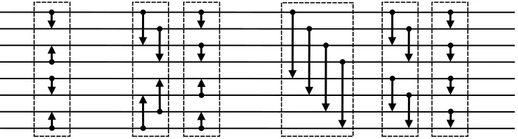
Proof. We use a variant of bitonic sort, introduced by Batcher [5]. It is well-known that, given a list of n elements, bitonic sort runs in O n·log2n

time. The algorithm, viewed as a sorting network, proceeds in O log2n iterations, where each iteration consists of n₂ comparators (see Figure1). In each iteration, the comparators are totally parallelizable, but our goal is to perform the comparatorsefficiently using standard word-level operation, i.e., to perform each iteration inO _Bn

standard word-level operations. The intuition is to pack sequentiallyO(B) elements into each word and then apply SIMD (single-instruction-multiple-data) comparators, where a SIMD comparator emulates O(B) standard comparators using only constant time. We show the following facts: (1) each iteration runs in O _Bn SIMD comparators andO _Bn time, and (2) each SIMD comparator can be instantiated by a constant number of word-level subtraction and bitwise operations.

Figure 1: A bitonic sorting network for 8 inputs. Each horizontal line denotes an input from the left end and output to the right end. Each vertical arrow denotes a comparator such that compares two elements and then swaps the greater one to the pointed end. Each dashed box denotes an iteration in the algorithm. The figure is modified from [65].

(18)

to show that it takes O(1) time to alignO(B) pairs of elements. By the definition of bitonic sort, in the same iteration, the offset between any compared pair is the same power of 2 (see Figure 1). Since B is also a power of 2, one of the following two cases holds:

(a) All comparators consider two elements from two distinct words, and elements are always aligned in the input.

(b) All comparators consider two elements from the same word, but the offset t between any compared pair is the same power of 2.

In case (a), the required alignment follows immediately. In case (b), it suffices to do the following:

1. Split one word into two words such that elements of the offset t are interleaved, where the two words are called odd and even, and then

2. Shift the even word byt elements so the comparators are aligned to the odd word.

The above procedure takesO(1) time. Indeed, there are two applications of the comparators, and thus it blows up the cost of the operation by a factor of 2. Thus, the algorithm of an iteration aligns elements, applies SIMD comparators, and then reverses the alignment. Every iteration runs

O _Bn SIMD comparators plusO _Bn time.

For fact (2), note that to comparek-bit strings it suffices to perform (k+ 1)-bit subtraction (and then use the sign bit to select one string). Hence, the intuition to instantiate the SIMD comparator is to use “SIMD” subtraction, which is the standard word subtraction but the packed elements are augmented by the sign bit. The procedure is as follows. Letkbe the bit-length of an element such that B ·k bits fit into one memory word. We write theB elements stored in a word as a vector

~a= (a1, . . . , aB)∈({0,1}k)B. It suffices to show that for any~a= (a1, . . . , aB) and~b= (b1, . . . , bB)

stored in two words, it is possible to compute the mask word m~ = (m1, . . . , mB) such that

mi =

(

1k ifai ≥bi

0k otherwise.

For binary stringsxandy, letxybe the concatenation ofxandy. Let∗be a wild-card bit. Assume additionally that the elements are packed with additional sign bits, i.e., ~a = (∗a1,∗a2, . . . ,∗aB).

This can be done by simply splitting one word into two. Consider two input words ~a = (1a1, 1a2, . . . ,1aB) and~b= (0b1,0b2, . . . ,0bB) such thatai, bi ∈ {0,1}k. The procedure runs as follows:

1. Let ~s0 ₌_~a₋_~b_{, which has the format} _s

1∗k, s2∗k, . . . , sB∗k

, where si ∈ {0,1} is thesign bit

such thatsi = 1 iffai≥bi. Keep only sign bits and let~s= s10k, . . . , sB0k

.

2. Shift~s and getm~0 _{= 0}k_s

1, . . . ,0ksB

. Then, the mask is m~ =~s−m~0 _{= 0}_sk

1, . . . ,0skB

.

The above takes O(1) subtraction and bitwise operations. This concludes the proof.

4.2 Oblivious Random Permutations

We say that an algorithm ORP is a statistically secure oblivious random permutation, iff ORP statistically obliviously simulates the functionality Fperm which, upon receiving an input array of

(19)

Theorem 4.3. Let n > 100 and let D denote the number of bits it takes to encode an element. There exists a (1−e−

√

n₎_{-oblivious random permutation for arrays of size} _{n. It runs in time}

O(T_sortD+logn(n) +n), where T_sort` (n) is an upper bound on the time it takes to sort n elements each of size ` bits.

Later, in our ORAM construction, this version of ORP will be applied to arrays of size n ≥

log3λ, whereλis a security parameter, and thus the failure probability is bounded by a negligible function inλ.

Proof of Theorem 4.3. We apply a similar algorithm as that of Chan et al. [11, Figure 2 and Lemma 10], except with different parameters:

• Assign each element an 8 logn-bit random label drawn uniformly from{0,1}8 logn_{. Obliviously}

sort all elements based on their random labels, resulting in the array R. This step takes

O(T_sortD+logn(n) +n) time.

• In one linear scan, write down two arrays: 1) an arrayIcontaining the indices of all elements that have collisions; and 2) an arrayXcontaining all the colliding elements themselves. This can be accomplished in O(n) time assuming that we can leak the indices of the colliding elements.

• If the number of elements that collide is greater than√n, simply abort throwing anOverflow exception. Otherwise, use a na¨ıve quadratic oblivious random permutation algorithm to obliviously and randomly permute the array X, and let Y be the outcome. This step can be completed in O(n) time where the quadratic oblivious random permutation performs the following: for each of i∈ {1,2, . . . , n}, sample a random index r from {1,2, . . . , n−i+ 1}, and write thei-th element of the input to ther-th unoccupied position of the output through a linear scan of the output array.

• Finally, for each j∈ |I|, write back each elementY[j] to the position R[I[j]] and output the resultingR.

To bound the probability ofOverflow, we first prove the following claim:

Claim 4.4. Letn >100. Fix a subsetS⊆ {1,2, . . . , n}of sizeα≥2. Throw elements{1,2, . . . , n}

to n8 _{bins independently and uniformly at random. The probability that every element in} _S _{has a}

collision with any other elements is upper bounded by α!/n2α.

Proof. If all elements in S see collisions for some sample path determined by the choice of all elements’ bins denotedψ, then the following eventGS must be true for the sample pathψ: there is a permutationS0 ofSsuch that for everyi∈ {dα/2e, . . . , α},S0[i] either collides with some element in S0 whose index j < i (i.e., with an element before itself) or with an element outside of S (i.e., from [n]\S).

Therefore, the fraction of sample paths for which a fixed subset S of size α all have collision is upper bounded by the fraction of sample paths over which the above eventGS holds. Now, the fraction of sample paths over which theGSholds is upper bounded byα!·(n/n8)bα/2c≤α!/n2α.

(20)

a subset S: n α · α!

n2α =

n! (n−α)!α!·

α!

n2α ≤

e√n(n/e)n

p

2π(n−α)((n−α)/e)n−α_·√₂_πα₍_α/e₎α ·

α!

n2α

≤e √

n

2π ·

nn

(n−α)n−α_·_αα ·

α!

n2α =

α!·e√n

2π ·

n n−α

n−α

· 1

αα ·

1

nα

≤α!·e √

n

2π ·

1 + α

n−α

n

· 1

αα ·

1

nα

Plugging inα=√n, we can upper bound the above expression as follows assuming largen >100:

√

n!·e√n

2π ·

1 +

√

n n−√n

√

n·√n

· 1

(n√n)√n ≤ √

n!·e√n

2π ·

1 + 1

0.5√n

0.5

√

n·2·√n

· 1

(n√n)√n

≤ √

n!·e√n

2π ·exp(2

√

n)· 1

(n√n)√n ≤exp(− √

n)

Having bounded the Overflowprobability, the obliviousness proof can be completed in identical manner to that of Lemma 10 in Chan et al. [11], since our algorithm is essentially the same as theirs but with different parameters. We stress the algorithm is oblivious even though the positions of the colliding elements are revealed.

Packed oblivious random permutation. The following version of oblivious random permu-tation has good performance when each memory word is large enough to store many copies of the elements to be permuted tagged with their own indices. The algorithm follows directly by plug-ging in our oblivious packed sort (Theorem 4.2) into the oblivious random permutation algorithm (Theorem4.3).

Theorem 4.5(Packed oblivious random permutation). Letn >100and letDdenote the number of bits it takes to encode an element. LetB=bw/(logn+D)c be the element capacity of each memory word and assume that B > 1. Then, there exists an (1−e−

√

n₎_{-oblivious random permutation}

algorithm that permutes the input array in time O _Bn ·log2n+n.

Perfect oblivious random permutation. Note that the permutation of Theorem 4.3runs in timeO(n·logn) but it may fail w.p.e−

√

n_{. We construct a}_perfectly_{oblivious random permutation in}

this paper. This scheme comes as a by-product of our tight compaction and intersperse algorithms that we construct later in Sections 5and 6.4.

Theorem 4.6 (Perfectly oblivious random permutation). For any n, any m ∈ [n], suppose that sampling an integer uniformly at random from [m] takes unit time. Then, there exists a perfectly oblivious random permutation such that permutes an input array of size nin O(n·logn) time.

Proof. We will prove this theorem in Section6.4.

4.3 Oblivious Bin Placement

Let I be an input array containing real and dummy elements. Each element has a tag from

(21)

in thei-th cell ofI0. If no element was tagged with a valuei, then I0[i] =⊥. The values in the tags of real elements can be thought of as “bin assignments” where the elements want to go to and the goal of the bin placement algorithm is to route them to the right location obliviously.

Oblivious bin placement can be accomplished withO(1) number of oblivious sorts (Section4.1), where each oblivious sort operates overO(|I|) elements [12,15]. In fact, these works [12,15] describe a more general oblivious bin placement algorithm where the tags may not be distinct, but we only need the special case where each tag appears at most once.

4.4 Oblivious Hashing

An oblivious (static) hashing scheme is a data structure that supports three operations Build, Lookup, andExtract that realizes the following (ideal) reactive functionality. The Buildprocedure is the constructor and it creates an in-memory data structure from an input array I containing real and dummy elements where each real element is a (key, value) pair. It is assumed that all real elements inI have distinct keys. TheLookup procedure allows a requestor to look up the value of a key. A special symbol⊥ is returned if the key is not found or if ⊥is the requested key. We say a (key, value) pair is visited if the key was searched for and found before. Finally, Extract is the destructor and it returns a list containing unvisited elements padded with dummies to the same length as the input array I.

An important property that our construction relies on is that if the input array I is randomly shuffled to begin with (with a secret permutation), the outcome ofExtractis also randomly shuffled (in the eyes of the adversary). In addition, we need obliviousness to hold only when the Lookup sequence is non-recurrent, i.e., the same real key is never requested twice (but dummy keys can be looked up multiple times). The functionality is formally given next.

Functionality 4.7: Fn

HT – Hash Table Functionality for Non-Recurrent Lookups

• Fn

HT.Build(I):

– Input: an array I= (ai, . . . , an) containing nelements, where each ai is eitherdummy

or a (key, value) pair denoted (ki, vi)∈ {0,1}D × {0,1}D.

– Assumption: throughout the paper, we assume that both the key and the value can be stored in O(1) memory words, i.e.,D=O(w) wherewdenotes the word size. – The procedure:

1. Initialize the state stateto (I,P), where P=∅. – Output: TheBuildoperation has no output.

• Fn

HT.Lookup(k):

– Input: The procedure receives as input a key k(that might be ⊥, i.e., dummy). – The procedure:

1. Parse the internal state asstate= (I,P).

2. Ifk∈P(i.e.,k is a recurrent lookup) then halt and outputfail. 3. Ifk=⊥ork /∈I, then set v∗ =⊥.

4. Otherwise, setv∗=v, wherev is the value that corresponds to the key k inI. 5. UpdateP=P∪ {(k, v)}.

(22)

• Fn

HT.Extract():

– Input: The procedure has no input. – The procedure:

1. Parse the internal statestate= (I,P).

2. Define an arrayI0 = (a0₁, . . . , a0_n) as follows. Fori∈[n], seta0_i=ai ifai = (k, v)∈/ P.

Otherwise, seta0_i=dummy. 3. ShuffleI0 uniformly at random. – Ouptut: The arrayI0.

Construction of na¨ıveHT. A na¨ıve, perfectly secure oblivious hashing scheme can be obtained directly [14,19] from a perfectly secure ORAM construction [14,19]. Both schemes [14,19] are Las Vegas algorithms: for any capacityn, it almost always takesO(log3n) time to serve a request — however with negligible in n probability, it may take longer to serve a request. We stress that although the runtime may sometimes exceed the stated bound, there is never any security or correctness failure in the known perfectly secure ORAM constructions [14,19]. We observe that the scheme of Chan et al. [14] is a Las Vegas algorithm only because the oblivious random permutation they employ is a Las Vegas algorithm. In this paper, we actually construct a perfect oblivious random permutation that runs in O(n·logn) time with probability 1 (Theorem 4.6). Thus, we can replace the oblivious random permutation in Chan et al. [14] with our own Theorem 4.6. Interestingly, this results in the first non-trivial perfectly oblivious RAM that is not a Las Vegas algorithm.

Theorem 4.8 (Perfect ORAM (using [14] + Theorem 4.6)). For any capacity n ∈ _N, there is a perfect ORAM scheme that consumes space O(n) and worst-case time overhead O log3n per request.

To construct na¨ıveHTusing perfectly secure ORAM scheme, we use Theorem 4.8to compile a standard, balanced binary search tree data structure (e.g., a red-black tree). Finally, Extractcan be performed in linear time if we adopt the perfect ORAM of Theorem 4.8 which incurs constant space blowup. In more detail, we flatten the entire in-memory data structure into a single array, and apply oblivious tight compaction (Theorem 1.2) on the array, moving all the real elements to the front. We then truncate the array at length |I|, apply a perfectly random permutation on the truncated array, and output the result. This gives the following construction.

Theorem 4.9(na¨ıveHT). Assume that each memory word is large enough to store at leastΘ(logn)

bits where n is an upper bound on the total number of elements that exist in the data structure. There exists a perfectly secure, oblivious hashing scheme that consumes O(n) space; further,

• Buildand Extract each consumes n·polylogn time;

• Each Lookup request consumespolylogntime.

(23)

4.5 Oblivious Cuckoo Hashing

A Cuckoo hashing scheme [52] is a hashing method with constant lookup cost (ignoring the stash). Imagine that we wish to hash n balls into a table of size ccuckoo ·n, where ccuckoo > 1 is an appropriate fixed constant. Additionally, there is a stash denoted S of size s for holding a small number of overflowing balls. We also refer to each position of the table as a bin, and a bin can hold exactly one ball. Each ball receives two independent bin choices. During the build phase, we execute a Cuckoo assignment algorithm that picks either a bin-choice for each ball among its two specified choices, or assigns the ball to some position in the stash. It must hold that no two balls are assigned to the same location either in the main table or in the stash. Kirsch et al. [39] showed an assignment algorithm that succeeds with with probability 1−n−Ω(s) over the random bin choices, wheresdenotes the stash size.

Without privacy, it is known that such an assignment can be computed inO(n) time. However, it is also known that the standard procedure for building a Cuckoo hash table leaks information through the algorithm’s access patterns [12,33,60]. Goodrich and Mitzenmacher [33] (see also the recent work of Chan et al. [12]11) showed that a Cuckoo hash table can be built obliviously

in O(n·logn) total time. In our ORAM construction, we will need to apply Chan et al. [12]’s oblivious Cuckoo hashing techniques in a non-blackbox fashion to enable asymptotically more efficient hashing schemes for randomly shuffled input arrays. Below, we present the necessary preliminaries.

4.5.1 Build Phase: Oblivious Cuckoo Assignment

To obliviously build a Cuckoo hash table given an input array, we have two phases: 1) a metadata

phase in which we select a bin among the two bin choices made by each input ball or alternatively assign the ball to a position in the stash; and 2) the actual (oblivious) routing of the balls into their destined location in the resulting hash-table data structure. The problem solved by the the first phase (i.e., the metadata step), is called the Cuckoo assignment problem, formally defined as below.

Oblivious Cuckoo assignment. Let nbe the number of balls to be put into the Cuckoo hash table, letI= ((u1, v1), . . .(un, vn)) be the array of the two bin choices made by each of the nballs,

whereui, vi∈[ccuckoo·n] fori∈[n]. In the Cuckoo assignment problem, given such an input array I, the goal is to output an array A={a1, . . . an}, where ai ∈ {bin(ui),bin(vi),stash(j)} denotes

that thei-th ball is assigned either to bin ui or binvi, or to the j-th position in the stash. We say

that a Cuckoo assignmentA is correct iff it holds that (i) each bin and each position in the stash receives at most one ball, and (ii) the number of balls in the stash is bounded by a parameter s.

Given a correct assignmentA, a Cuckoo hash table can be built by obliviously placing the balls into the position it is assigned too. A straightforward way to accomplish this is through a standard oblivious bin placement algorithm (Section 4.3)12.

Theorem 4.10 (Oblivious Cuckoo assignment [12,33]). Let ccuckoo>1be a suitable constant, δ > 0,n∈N, the stash size s≥log(1/δ)/logn, and letncuckoo :=ccuckoo·n+sand`:= 8 log2(ncuckoo).

11

Chan et al. [12] is a re-exposition and slight rectification of the elegant ideas of Goodrich and Mitzenmacher [33]; also note that the Cuckoo hashing appears only in the full version of Chan et al.,http://eprint.iacr.org/2017/924.

12

OptORAMa: Optimal Oblivious RAM

OptORAMa: Optimal Oblivious RAM

Contents

1

Introduction

2

Technical Roadmap

3

Preliminaries

4

Oblivious Building Blocks