Rational Expectations for Large Models: A Practical Algorithm and a Policy Application

Full text

(1)Eleventh Floor Menzies Building PO Box 11E, Monash University Wellington Road CLAYTON Vic 3800 AUSTRALIA. CENTRE of POLICY STUDIESand the IMPACT PROJECT. Telephone: (03) 9905 2398, (03) 9905 5112. from overseas: 61 3 9905 5112 or 61 3 9905 2398. Fax: (03) 9905 2426 e-mail web site. 61 3 9905 2426 [email protected] http://www.monash.edu.au/policy/. RATIONAL EXPECTATIONS FOR LARGE MODELS: A PRACTICAL ALGORITHM AND A POLICY APPLICATION by. Peter B. DIXON, K. R. PEARSON, MARK R. PICTON and. Maureen T. RIMMER Centre of Policy Studies, Monash University. Preliminary Working Paper No. IP-81, May 2003 ISSN 1 031 9034. ISBN 0 7326 1538 0. The Centre of Policy Studies (COPS) is a research centre at Monash University devoted to quantitative analysis of issues relevant to Australian economic policy..

(2)

(3) Abstract This paper describes a practical and conceptually simple iterative method for solving large dynamic CGE models under rational expectations. Details are given for the MONASH model of Australia but the general approach could be applied to a wide range of dynamic models. The method has been automated in the RunMONASH Windows software. This software provided a natural starting point for developing an automated procedure for conducting policy analysis under rational expectations because it already performed this function for static expectations. RunMONASH was also convenient because it incorporates comprehensive user-friendly data- and solution-interrogation facilities.. We provide an illustrative application in which. MONASH results obtained under rational expectations for the effects of motor vehicle tariff cuts are compared with results obtained under static expectations. JEL classifications: C53, C63, C68, F14 Key words: rational expectations algorithm, dynamic general equilibrium, tariffs, investment modelling. i.

(4) ii.

(5) Contents Abstract. i. 1. Introduction. 1. 2. The MONASH algorithm for conducting simulations under rational expectations 2.1 Static versus rational expectations 2.2 Usual methods of handling non-recursive computations 2.3 The iterative method for solving MONASH under rational expectations 2.3.1 EROR(j,t) in the different iterations of rational-expectations simulations. 3. 4. 1 1 3 4 4. 2.4. Using RunMONASH to conduct rational-expectations simulations 2.4.1 RunMONASH with rational expectations 2.4.2 Demonstration version of RunMONASH 2.4.3 Models other than MONASH. 6 7 8 8. 2.5. Convergence and computer time. 8. The effects of cuts in motor vehicle tariffs under static and rational expectations. 10. 3.1. Key assumptions 3.1.1 Labour market 3.1.2 Public expenditure and taxes 3.1.3 Private consumption 3.1.4 Adjustment of capital and expected rates of return 3.1.5 Production technologies 3.1.6 The numeraire. 10 11 11 12 12 12 12. 3.2. Results 3.2.1 Static expectations 3.2.2 Rational expectations 3.2.3 Conclusions about adjustment paths17. 12 12 15. Concluding remarks. 17. References. 18. iii.

(6) Figure, Table and Charts Figure 2.1. Convergence of the algorithm for imposing rational expectations. Table 2.1. Year-on-year growth rates for real aggregate investment for selected iterations in the basecase forecast from 2002 to 2016 (ADJ_RE = 0.2). 19. Policy effects on real aggregate investment with ADJ_RE = 0.3 and 30 basecase iterations: 5, 10 and 20 policy iterations. 19. Year-on-year growth rates for real aggregate investment for selected iterations in the basecase forecast. 20. Cumulative growth paths for real aggregate investment for selected iterations in the basecase forecast. 20. Real aggregate investment in selected iterations of the basecase forecast. 21. Chart 2.5. Policy effects on real aggregate investment. 21. Chart 3.1. Aggregate employment. 22. Chart 3.2. Aggregate capital stock. 22. Chart 3.3. Real wage rate. 23. Chart 3.4. Real aggregate investment. 23. Chart 3.5. Real aggregate private consumption. 24. Chart 3.6. Terms of trade. 24. Chart 3.7. National savings as a share of GNP. 25. Chart 3.8. Real exchange rate. 25. Chart 3.9. Aggregate export volumes. 26. Chart 3.10. Real GDP. 26. Chart 3.11. Aggregate import volumes. 27. Chart 3.12. Index of asset prices of capital. 27. Chart 2.1. Chart 2.2 Chart 2.3 Chart 2.4. iv. 6.

(7) Rational Expectations for Large Models: a Practical Algorithm and a Policy Application Peter B. Dixon, K.R. Pearson, Mark R. Picton and Maureen T. Rimmer Centre of Policy Studies, Monash University, Clayton 3800, Australia May 15, 20031 1. Introduction. In most dynamic models, investment in any year depends on the expected rates of return on investment carried out in that year. Under static expectations, the expected rate of return is derived from current or past values for rental rates, asset prices, taxes, interest rates and other relevant variables. With static expectations, a model can be solved recursively (that is, one year at a time). Under rational expectations, the expected rate of return is the actual rate of return. Calculation of the actual rate of return in any year requires information from the next year on rental rates, asset prices and other variables. Thus, it is not possible to solve a model recursively under rational expectations. We cannot solve the model in year 1 until we know rental rates, asset prices etc. for year 2. Thus, the solution for year 1 requires the solution for year 2. But the solution for year 2 requires the solution for year 1 to set initial conditions. This two-way interdependence of solutions makes rational expectations computationally difficult in a large model. This paper describes a practical and conceptually simple iterative method for solving large models under rational expectations. Details are given for the MONASH model of Australia. However, the general approach could be applied to a wide range of dynamic models. The paper also provides an illustrative application in which MONASH results obtained under rational expectations for the effects of motor vehicle tariff cuts are compared with results obtained under static expectations. The iterative method described here was initially designed and implemented by Dixon and Rimmer (2001 and 2002). Experience in its application has been reported by Adams (2000) and Adams, Andersen and Jacobsen (2001). As reported in this paper, the method has now been automated in the RunMONASH Windows software. RunMONASH provides a natural starting template for developing an automated procedure for conducting policy analysis under rational expectations because (a) it was designed to automate and compare basecase forecast simulations and alterative policy simulations under static expectations and (b) it incorporates comprehensive user-friendly data- and solution-interrogation facilities. Interested readers can download the Demonstration Version of RunMONASH and the relevant files for replicating both the static and rational versions of the motor vehicle tariff application.2 2 2.1. The MONASH algorithm for conducting simulations under rational expectations Static versus rational expectations. Like most other dynamic models, for MONASH investment in any year depends on the expected rate of return on investment made in that year. The equation takes the form: 1. This is a revised version of a paper presented in June 2003 at the Sixth Annual Conference on Global Economic Analysis in The Netherlands. 2 See http://www.monash.edu.au/policy/gprmon1.htm . Further details are given in subsection 2.4.2..

(8) INV(j,t) = F(EROR(j,t), plus other variables). (2.1). where INV(j,t) is the rate of investment in industry j in year t; EROR(j,t) is the expected rate of return on investment in industry j in year t; and F is an increasing logistic function. The logistic functional form, with its lower and upper bounds, was chosen for investment to avoid unrealistically large fluctuations in simulated capital growth rates. The natural lower bound for the rate of investment in any industry is the negative of the rate of depreciation in that industry. The upper bound is somewhat arbitrary. It is set in MONASH so that an industry’s rate of capital growth in any year cannot be more than 6 percentage points above the industry’s historically normal rate of growth. Thus, for example, if the historically normal rate of capital growth in an industry is 3 per cent, then we impose an upper limit on its simulated capital growth in any year of 9 per cent. Under rational expectations EROR(j,t) is defined according to EROR(j,t) = ROR_ACT(j,t). (2.2). where ROR_ACT(j,t) is the actual rate of return in industry j in year t. In determining ROR_ACT(j,t) we start by calculating the present value [PV(j,t)] of purchasing in year t a unit of capital for use in industry j3: PV ( j, t ) = − PI( j, t ) +. Q( j, t + 1) + PI( j, t + 1) * [1 − D( j)] 1 + INT. (2.3). where PI(j,t) is the cost of buying or constructing in year t a unit of capital for use in industry j; D(j) is the rate of depreciation in industry j; Q(j,t) is the rental rate on j’s capital in year t, i.e. the user cost of a unit of capital in year t; and INT is the nominal rate of interest which is assumed to be constant here (but not in MONASH). In (2.3) we assume that the acquisition in year t of a unit of physical capital in industry j involves an immediate outlay of PI(j,t) followed in year t+1 by two benefits which must be discounted by one plus the interest rate. The first benefit is the rental value, Q(j,t+1), of an extra unit of capital in year t+1. The second is the value, PI(j,t+1)*[1-D(j)], at which the depreciated unit of capital can be sold in year t+1. To derive a rate-of-return formula we divide both sides of (2.3) by PI(j,t), i.e., we define the actual rate of return in year t on physical capital in industry j as the present value of an investment of one dollar. This gives  1   Q(j, t + 1)   1 - D(j)   PI(j, t + 1)   +   . ROR_ACT(j, t) = −1 +   *   *   1 + INT   PI(j, t)   1 + INT   PI(j, t) . (2.4). Thus, under rational expectations, investors make decisions in year t on the assumption that capital rentals and asset prices will change between years t and t+1 in the way indicated by our model. Under static expectations, EROR(j,t) is defined according to. 3. Here we ignore taxes on capital. They are not ignored in MONASH.. 2.

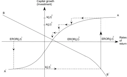
(9) EROR(j,t) = EROR_SE(j,t). (2.5). where EROR_SE(j,t) is the static expectation of the actual rate of return in industry j in year t. Under static expectations, decisions in year t to adjust capital stocks are made on the assumption that capital rentals [Q(j,t)] and asset prices [PI(j,t)] will grow between years t and t+1 at the current rate of inflation (INF).4 Under these assumptions, it follows from (2.4) that 1    Q(j, t)   1 - D(j)   +  EROR_SE(j, t) = −1 +   *    1 + RINT   PI(j, t)   1 + RINT . (2.6). where RINT is the real interest rate [= (1+INT)/(1+INF)]. Thus, under static expectations, investment decisions in each industry in year t are heavily influenced by current profitability. Clearly a recursive solution procedure will work under static expectations [when (2.5) and (2.6) hold] but not under rational expectations [when (2.2) and (2.4) hold]. For simulations under static expectations, information about the expected rates of return in year t is available when the solution for year t is calculated. However, for simulations under rational expectations, information about the expected rates of return in year t is not available when the solution for year t is calculated. This is because knowledge of the actual rate of return in year t requires values of the capital rentals and asset prices in year t+1. 2.2. Usual methods of handling non-recursive computations. There are two broad strategies for handling non-recursive computations. The first is to solve all years simultaneously. This simultaneous-solution method for dynamic models was recognized by Wilcoxen (1985 and 1987) and Bovenberg (1985). It has been used recently by Malakellis (2000) for a 13 sector model. For more details, see section 2.1(a) of Dixon and Rimmer (2002) and Chapter 5 of Dixon et al (1992). A disadvantage of the simultaneous-solution method is that it is feasible only if the underlying model is small. When a model is solved simultaneously, the size of the system of equations to be solved is multiplied by N where N is the number of years in the simulation period. For large models like MONASH (which has over 100 industries) it is not possible to solve simultaneously over 15 or so years (even on modern PCs with large memory). Another disadvantage of the simultaneous-solution method is that it requires the addition of a time dimension throughout the algebraic representation of the model. This involves set-up costs and lowers the transparency of the model equations for the human reader. The second broad strategy for handling non-recursive computations is to adopt an iterative method. Iterative methods have the advantage that they do not require the addition of a time dimension throughout the model. Early iterative methods include single and multiple shooting algorithms5 [see Chapter 5 of Dixon et al (1992) for details]. At each step, these algorithms use guesses of shadow prices of capital stocks (variables whose true values cannot be known independently of model solutions for later years) for the first year of a simulation and a limited number of subsequent years. The guesses are then refined in light of discrepancies in earlier iterations between implied values of shadow prices and either guessed values or known terminal values. However, shooting algorithms are not practical for a model like MONASH with over 100 industries, each with its own capital stock and investment. A more promising approach is the Fair-Taylor algorithm6 in which shadow prices are guessed for every year. The iterative method developed for MONASH is reminiscent of the Fair-Taylor algorithm. 4. As for the interest rate, the inflation rate is assumed to be constant here (but not in MONASH). The shooting algorithm is explained in Press et al. (1986) and Roberts and Shipman (1972). Details of a refinement, multiple shooting, are given in Lipton et al. (1982) and Roberts and Shipman (1972). 6 This algorithm was proposed by Fair (1979) and later extended by Fair and Taylor (1983). 5. 3.

(10) 2.3. The iterative method for solving MONASH under rational expectations. The iterative method developed to solve the MONASH model (or other large models) under rational expectations is documented in section 21 of Dixon and Rimmer (2002) and, in more detail, in sections 30.2 and 44 of Dixon and Rimmer (2001). Before giving details of the MONASH iterative method for rational expectations we require some background information on how MONASH policy applications are conducted. In running such applications we first construct a business-as-usual basecase forecast for each year in the simulation period. Then an alternative forecast, which includes the policy shocks, is run. This alternative forecast is called the policy forecast. The effects of the policy are then measured by the differences between the policy forecast and the basecase forecast. In each year of the basecase or policy forecast the model must be told how to calculate expected rates of return [EROR(j,t)]. Under static expectations EROR(j,t) is simply the static expectation of the actual rate of return [EROR_SE(j,t)] given in (2.6). In our iterative method for solving MONASH under rational expectations, EROR(j,t) must be set for each iteration of the basecase and policy forecasts. Below we provide details of our iterative method using the notation of subsection 2.1. Note that the addition of a time dimension here and in section 2.1 is for ease of presentation only. Unlike the simultaneous method, the MONASH iterative method does not require the addition of a time dimension throughout the algebraic representation of the model. 2.3.1. EROR(j,t) in the different iterations of rational-expectations simulations. In the first iteration of the basecase forecast, EROR(j,t) is set equal to the static expectation of the rate of return: EROR(j,t) 1 = EROR_SE(j,t) 1. (2.7). where the superscripts denote the iteration number. After the first iteration, actual rates of return are known from the previous iteration for each year except the last. The actual rates of return are not known for the last year since these depend on rental rates and asset prices beyond the simulation period. In the second iteration of the basecase forecast for each year except the last, T , EROR(j,t) is set equal to the actual rate of return from the first iteration, the idea being that as soon as we have some estimates of actual rates of return, they should be used: EROR(j,t) 2 = ROR_ACT(j,t) 1. (2.8). for all years t < T. We adopt the terminal condition that expected rates of return in year T are the same as in the previous year: EROR(j,T) 2 = EROR(j,T-1) 2 .. (2.9). In the third and subsequent iterations of the basecase forecast, we set EROR(j,t) n = EROR(j,t) n-1 + ADJ_RE(j)*[ROR_ACT(j,t) n-1 – EROR(j,t) n-1]. (2.10). for all years t < T, and EROR(j,T) n = EROR(j,T-1) n. (2.11). 4.

(11) where ADJ_RE(j) is an adjustment parameter set between 0 and 1. Unlike the second iteration where we adopted for expected rates of return the actual rates of return emerging from the first iteration, in the third and subsequent iterations we take a more cautions approach, only partially revising the previous iteration’s expected rates of return in light of the actual rates of return emerging from that iteration. We do this to avoid cycling in simulations under rational expectations. Figure 2.1 and the accompanying text discusses cycling and partial adjustment. While high values of ADJ_RE(j) can lead to cycling, low values make convergence too slow. Experience has shown that satisfactory convergence is achieved with ADJ_RE(j) set equal to 0.2 or 0.3 for each industry j. Convergence is achieved at iteration number N if EROR(j,t) N = ROR_ACT(j,t) N for all j and t < T.. (2.12). Exact equality between EROR and ROR_ACT is not likely to be achieved. In practice, it is appropriate to stop iterating once the differences between EROR(j,t) and ROR_ACT(j,t) are suitably small. It is possible to look at these differences after each iteration. If the differences are not sufficiently small, more iterations can be undertaken. After convergence has been achieved for the basecase forecast in N iterations, the policy forecast can be conducted. However, before carrying out policy simulations, we have found that it is desirable to use the policy closure in a re-computation of the final forecast iteration. In this forecast re-run (iteration N+1), all of the exogenous variables are given the values that they had, either exogenously or endogenously, in the final forecast iteration. This means that expected rates of return in iteration N+1 are set at the same values that they had in iteration N: EROR(j,t) N+1 = EROR(j,t) N .. (2.13). In theory, the forecast re-run iteration should produce the same results as the final forecast iteration. In practice, the results will differ slightly because of different linearization errors produced under different closures.7 By adopting the forecast re-run as the simulation from which we calculate policy-induced deviations, we minimize the possibility that these deviations will be contaminated by differences in linearization errors in the forecast and policy simulations.8 In the first iteration of the policy forecast (iteration N+2), we use the rational-expectations basecase forecast to advise our opening guess of expected rates of return. We set EROR(j,t) N+2 = EROR(j,t) N+1 + [EROR_SE(j,t) N+2 – EROR_SE(j,t) N+1]. (2.14). for all years t < T and EROR(j,T) N+2 = EROR(j,T-1) N+2.. (2.15). 7. They are also different because of the path dependency of the Divisia price and quantity indexes used in MONASH (see section 20 of Dixon and Rimmer, 2002). 8 All results reported in this paper were obtained using 4 Euler steps (see section 1.1 of Dixon and Rimmer, 2002). We checked that the associated linearization errors are not significant by redoing the calculations with 8 Euler steps, which produced results which were not significantly different from those obtained using 4 Euler steps.. 5.

(12) Figure 2.1. Convergence of the algorithm for imposing rational expectations Capital growth (Investment) B. A. 2. k(j,t). 3. k(j,t). 3. 1. EROR(j,t). EROR(j,t). 2. EROR(j,t). Rates of return. 1. k(j,t) /. A. B. /. We assume for convenience here (but not in MONASH) that there is no disequilibrium in expected rates of return. Thus, MONASH outcomes for expected rates of return and rates of capital growth (investment) in year t in industry j are on the AA′ schedule described in (2.1). We also assume that MONASH outcomes for actual rates of return and rates of capital growth are on the BB′ schedule. In drawing BB′ we have in mind the capital demand equation for year t+1 which, other things being equal, implies a negative relationship between the availability of physical capital to industry j in year t+1 and its rental rate in year t+1, and thus a negative relationship between capital growth in year t and the actual rate of return in year t. In MONASH computations, BB′ moves between iterations and we do not necessarily operate on AA′. Nevertheless, Figure 1 is a useful device for thinking about the convergence of our algorithm. For example, with the AA′ and BB′ curves in our figure, convergence described in (2.8) and (2.10) is very rapid when ADJ_RE(j) is set at 0.3 (the illustrated case). If ADJ_RE(j) is set at 1.0, then readers will find, after a little experimenting with the figure, that the algorithm may become stuck in a non-converging cycle, or converge very slowly. This occurs in practice – see section 2.5 below.. That is, we assume for t < T that the expected rate of return is the actual rate of return from the rerun version of the basecase forecast [EROR(j,t) N+1= ROR_ACT(j,t) N+1] amended by the effect of the policy on the static version of the expected rate of return [EROR_SE(j,t) N+2 – EROR_SE(j,t)N+1]. After the first policy iteration, expected rates of return in the policy simulation follow the pattern described in (2.8) to (2.11) for the basecase forecast until convergence is reached. 2.4. Using RunMONASH to conduct rational-expectations simulations. The iterative method for conducting policy applications under rational expectations has now been automated in RunMONASH. RunMONASH is a Windows interface which automates the setting up and solving of multi-year simulations carried out with general equilibrium models implemented and solved using GEMPACK (Harrison and Pearson, 1996). When a recursive dynamic model is solved using RunMONASH, the user needs to specify the model, the starting data files, the start and end years of the simulation period (for example, 2001 and 2016), and the closure and shocks for each year. The software then solves the model across the required years and makes the results available in a Windows format.. 6.

(13) When working with MONASH, it is usual to carry out three forecast runs, as follows: •. first, the basecase forecast. In conducting this forecast we adopt everything we think we know about the future including: volumes and prices of agricultural and mineral products forecast by the Australian Bureau of Agricultural and Resource Economics; numbers of international tourists forecast by the Bureau of Tourism Research; most macro variables forecast by macro specialists such as Access Economics and the Australian Treasury; and numerous disaggregated taste and technology variables extrapolated from MONASH historical simulations. All these variables are exogenized and shocked. To allow these variables to be exogenous we must endogenize many naturally exogenous variables such as the positions of foreign demand curves, the positions of domestic export supply curves and macro coefficients such as the average propensity to consume.. •. second, the forecast re-run. As mention in subsection 2.3, the forecast re-run is a repeat of the basecase forecast but is obtained by adopting the policy closure and setting all exogenous variables at their values in the basecase forecast simulation.. •. third, the policy forecast. In this simulation we introduce the policy shocks. To accommodate the policy shocks we require a different closure to that used in the basecase forecast. All the variables that could be affected by the policy shock (such as exports of agricultural and mineral products, tourism exports and macro variables) are endogenized. Correspondingly, naturally exogenous variables (such as the positions of foreign demand curves, the positions of domestic export supply curves and macro coefficients) are exogenized. In the policy forecast all the exogenous variables are shocked with their basecase forecast values with the exception of the policy variables which are shocked with their policy values rather than their forecast values.. The effect of the policy is then measured by the deviations between the policy forecast and the basecase forecast (re-run). As illustrated in the charts in section 3, we usually express the effects of the policy via the cumulative percentage deviations from basecase forecast values. For example, in Chart 3.1 we see that under static expectations the assumed reductions in motor vehicle tariffs reduced aggregate employment in 2005 by 0.027 per cent relative to its basecase forecast value. RunMONASH automatically produces spreadsheets and graphs of deviation results as well as yearon-year and cumulative results for the basecase, re-run and policy forecasts. 2.4.1. RunMONASH with rational expectations. To carry out applications under rational expectations, RunMONASH needs to be told how many iterations are wanted for each of the basecase and policy forecasts. The only additional requirements are (a) to choose values for the adjustment parameters ADJ_RE(j) in (2.10) and (b) to make two closure changes which allow the expected rates of return to be set according to the iterative method described in subsection 2.3.1. Then RunMONASH automates the calculations. When the simulations are complete, the results (spreadsheets and graphs) are available in the usual way. RunMONASH also provides information which can be used to determine if convergence has been satisfactory. For example, RunMONASH makes available tables showing the values of key variables (such as real aggregate investment, investment by industry and expected rates of return) in each of the last few iterations. The user can make a judgement about convergence on the basis of this information. If the user decides that convergence has not been adequate, RunMONASH can be asked to do more iterations.. 7.

(14) 2.4.2. Demonstration version of RunMONASH. The Demonstration Version of RunMONASH incorporating rational expectations can be downloaded from the web at address http://www.monash.edu.au/policy/gprmon1.htm Readers who download the demonstration version and associated files can carry out the motor vehicle tariff application under both static and rational expectations with a 32-sector version of the MONASH model. Instructions for running RunMONASH are available on the web. No GEMPACK licence is required to carry out these applications. 2.4.3. Models other than MONASH. RunMONASH is set up to handle rational expectations for the standard MONASH model, as documented in Dixon and Rimmer (2002 and 2001). RunMONASH can also be used to carry out rational-expectations simulations with other models provided they follow the standard MONASH nomenclature in a few ways. In particular, these other models must: •. use the same principles as MONASH for determining expected rates of return in iterations under rational expectations; and. •. have data files called ROREXT, EXTRA and ITER with much the same properties as those in the standard MONASH model. [These files contain data associated with investment and rational-expectations iterations. They do not contain the main input-output data for the model.]. The requirements for other models are documented fully in the topic “Model and Data Prerequisites” in the RunMONASH Help file. This Help file is part of the Demonstration Version of RunMONASH. 2.5. Convergence and computer time. The number of iterations required with the MONASH algorithm to achieve satisfactory convergence in a rational-expectations simulation depends on the setting of the adjustment parameters ADJ_RE(j). A low value of ADJ_RE(j) means that convergence is too slow (requiring a lot of iterations and time) and a high value for ADJ_RE(j) can lead to cycling with very slow convergence or failure to converge. In the motor vehicle tariff experiment reported in section 3 we set ADJ_RE(j) = 0.2 for each industry j and following a cautious approach performed 50 basecase forecast iterations followed by the forecast re-run simulation and 40 policy iterations. Very tight convergence was achieved for both the basecase forecast (see Table 2.1) and policy simulations. On experimenting with other values of ADJ_RE(j) we found that: •. with ADJ_RE(j) = 0.3, 30 basecase iterations and 20 policy iterations produced results that were indistinguishable from those reported in section 3;. •. with ADJ_RE(j) = 0.1 convergence was too slow;. •. with ADJ_RE(j) = 0.4 or 0.7, there was evidence of cycling, as expected from Figure 2.1 (more cycling and slower convergence with 0.7 than with 0.4); and. •. with ADJ_RE(j) = 0.8 or 0.9 the results did not converge, exhibiting non-damped cycles.. 8.

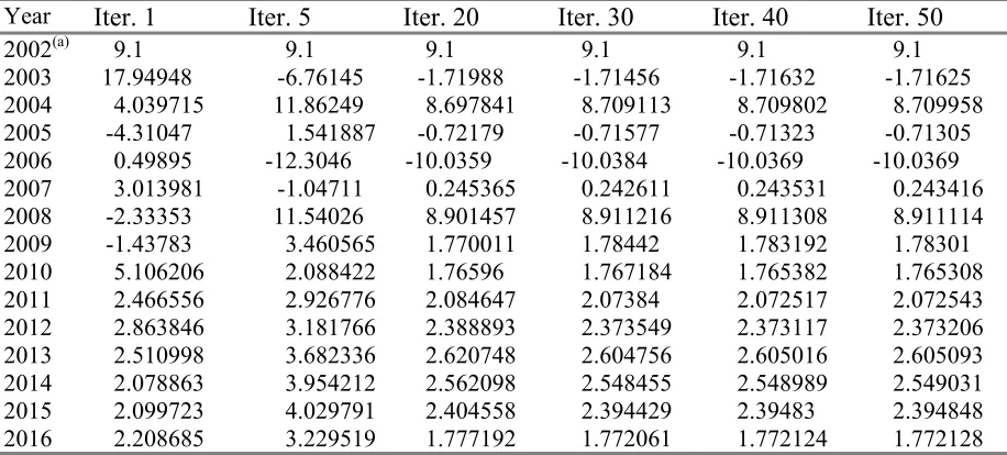
(15) Chart 2.1 shows cumulative deviation results for real aggregate investment9 generated in the experiment described in section 3 with ADJ_RE(j) = 0.3 for all j, 30 basecase forecast iterations and 5, 10 and 20 policy iterations. The 20 policy-iteration line is indistinguishable from the fully converged rational-expectations line in Chart 3.4 obtained with ADJ_RE(j) = 0.2 for all j, 50 basecase forecast iterations and 40 policy iterations. The 10-iteration line is barely distinguishable from the 20-iteration line but the 5-iteration line isn’t close enough. With a 30-iteration basecase, a forecast re-run and 20 policy iterations, a rational-expectations solution takes around 17 times as long as a static-expectations solution (1 basecase, 1 forecast rerun and 1 policy). For an application covering 20 years, rational-expectations policy applications for the 113 industry version of MONASH can be computed from scratch on a modern PC in about 10 hours. For the 32 sector version of MONASH, this time is brought down to about an hour and a half. Why do we conduct more iterations in the basecase forecast than in the policy forecast (30 compared with 10 or 20)? The reason is that very tight convergence is required in the basecase forecast simulation. If tight convergence has not been achieved, then the subsequent policy iterations pick up more than the effects of the policy shocks. Assume for example that the policy shocks are zero. Then if tight convergence were not achieved in the basecase forecast, in the policy forecast we would still observe differences between the policy results and the results in the final forecast iteration. But these would not reflect the effects of the policy. Rather they would reflect the ongoing movement towards a converged rational-expectations solution. Moreover, the converged rational-expectations policy forecast obtained in this way is different from the forecast obtained if the basecase simulation were allowed to continue to tight convergence. This is due to closure differences between the basecase forecast and the policy forecast. As soon as the policy forecast is started the exogenous shocks are fixed for all years of the simulation. The exogenous variables in the policy forecast are shocked in each year with the values they had in the corresponding year in the final iteration of the basecase forecast (the forecast re-run). Thus, if the basecase were terminated prior to convergence, the policy forecast would pick up wrong values for those exogenous variables that were endogenous in the basecase forecast and converge to a wrong rational-expectations policy solution. How fussy then do we need to be with basecase forecast convergence? We illustrate with an example from the tariff application in section 3. Table 2.1 shows year-on-year growth rates for aggregate investment in iterations 1, 5, 20, 30, 40 and 50 in the basecase forecast used in section 3, with ADJ_RE(j) = 0.2 for all j. (These results are readily available in RunMONASH.) In Chart 2.2 we sketch the results from Table 2.1. A quick glance at the chart will convince the reader that convergence is not achieved after 1 or 5 iterations, but maybe 20 iterations is enough as the growth rates for investment after 20, 30, 40 and 50 iterations are practically indistinguishable. Perhaps year-on-year growth rates are deceiving. Can we distinguish between iterations 20 to 50 using cumulative growth paths? These are plotted in Chart 2.3 for iterations 20, 30, 40 and 50. Again the answer is no, the paths are indistinguishable. However, it turns out that the visual checks in Charts 2.2 and 2.3 are not enough. A legitimate way to work out whether 20, 30 or 40 iterations is sufficient for the basecase forecast is to look at the cumulative deviation paths of investment in iterations 20, 30 and 40 from the path in iteration 50 (Chart 2.4). This gives a direct measure of the error in not continuing the forecast beyond 20, 30 or 40 iterations. For example, if the basecase forecast were stopped at 20 iterations 9. Real aggregate investment is a good macro variable to study because expected rates of return drive investment decisions. Investment variables are the most sensitive to the number of iterations and to the size of ADJ_RE(j). If aggregate investment or, better still, investment by industry results have converged, all other results will have converged.. 9.

(16) instead of 50, then the basecase forecast path for investment would have deviated from the fully converged basecase forecast (50 iterations) by amounts around a tenth the size of the investment deviations in the policy results (compare the scales in Charts 2.4 and 3.4).10 For the purposes of understanding and explaining results this level of accuracy may not be enough. Again comparing Charts 2.4 and 3.4 we conclude that 30 iterations is probably enough and 40 iterations is certainly enough. Chart 2.5 confirms the danger of not adequately converging in the basecase forecast. It shows two paths of investment deviations for the experiment discussed in section 3. One path is the correct solution in which both the basecase and policy forecasts are fully converged. In generating the other path we terminated the basecase forecast at 20 iterations and fully converged the policy forecast. As can be seen from the chart, failure to fully converge the basecase produces noticeable errors. 3. The effects of cuts in motor vehicle tariffs under static and rational expectations. In this section we use MONASH to look at the effects of cuts in the tariff on Motor Vehicles and Parts (MV&P) from 11.69 per cent in 2001, to 9.83 percent in 2002, to 7.97 per cent in 2003, to 6.11 per cent in 2004 and finally to 4.25 per cent in 2005 and subsequent years. This path of tariff reductions was recommended to the Government by the Australian Productivity Commission. The results presented are for the 32-sector version of MONASH. 3.1. Key assumptions. In our simulations we compute the effects of the proposed tariff cuts by comparing a policy simulation (which includes the tariff cuts) with a basecase forecast simulation in which the MV&P tariff rate is held at 11.69 per cent in all years. We conduct two policy simulations. In both the simulations the tariff cuts are unanticipated prior to the implementation of the first cut in 2002. Consequently the economy does not react to them until 2002. In the first policy simulation we assume that expectations of rates of return in each year are static, that is EROR for each industry is determined in (2.5) and (2.6). While the assumption of static expectations may be acceptable for most industries in the current application, it is not satisfactory for the MV&P industry. The key factors determining actual rates of return for this industry in the policy simulation over the period 2002 to 2005 are the tariff cuts. The path of these cuts is known in 2002 and therefore would be anticipated by people contemplating investment in MV&P capital. In the second policy simulation we assume that expectations are rational, that is EROR for each industry is determined in (2.2) and (2.4). Thus, in the second policy simulation, the path of tariff cuts are anticipated from 2002 onwards by investors in the MV&P industry. By comparing results from the first and second policy simulations we can see the effects of changes in our assumptions concerning rate-of-return expectations. To facilitate this comparison, it is important that the two policy simulations differ only because of the switch in the expectation assumption. Thus, the two policy simulations are conducted as deviations from identical basecase forecasts.11 10. It is tempting to think that if the basecase forecast was stopped at 20 iterations then the deviation path for investment would have been the path in Chart 3.4 lowered by the amount of the deviation path for Iter. 20 in Chart 2.3. This is not true however due to the fact that a fully rational expectations policy forecast obtained after a 20 iteration basecase is different to a fully rational expectations policy forecast obtained after tight convergence of the basecase (see the discussion of tight convergence earlier in subsection 2.5). 11 The static expectations policy simulation is the first policy iteration in our rational expectations algorithm and the rational expectations policy simulation is the 40th policy iteration (a fully converged rational solution). For both policy. 10.

(17) The key assumptions underlying both our policy simulations are as follows. 3.1.1. Labour market. We assume that real wage rates are sticky in the short run and flexible in the long run. This means that cuts in motor vehicle tariffs can lead to changes in aggregate employment in the short run. However, in the long run we assume that real wage rates adjust so that the tariff cuts have no effect on aggregate employment. This approach to the labour market is consistent with conventional macro-economic modelling in which the NAIRU (non-accelerating-inflation rate of unemployment) is exogenous. The parameters of our wage function are set so that the effects on aggregate employment of policy shocks are almost completely eliminated after five years. 3.1.2. Public expenditure and taxes. We assume that reductions in the MV&P tariff make no difference to the path of real public consumption and that the Government imposes an additional uniform consumer tax designed mainly to replace the lost tariff revenue. However, we assume that the Government is concerned not only with budgetary issues but also with short-run employment issues and the long-run wealth of the nation. To encapsulate all this, we include in MONASH the equation12:    E( t )  NSS(t - 1)   NSS( t )  − 1 − 1 + β − 1 = α  NSSf ( t − 1)   E f ( t )   NSSf ( t ) . (3.1). where NSS(t) is the share in year t of national savings13 in GNP in the policy simulation; NSSf(t) is the share in year t of national savings in GNP in the forecast simulation; E(t) and Ef(t) are the levels in year t of aggregate employment in the policy and forecast simulations; and α and β are positive parameters with α less than 1.14 Through (3.1) we allow the Government in policy simulations to relax its fiscal stance if employment in the policy simulation falls below its forecast level. In the first year of a policy simulation the first term on the RHS of (3.1) is zero. Thus, under (3.1), if the policy reduces aggregate employment then the Government allows the national savings share of GNP to fall below simulations, the basecase forecast is the policy re-run (a fully converged rational forecast, with the rational expectations policy closure). In interpreting the re-run as the basecase for the static policy simulation we recognise that although it was produced under rational expectations, it could have been produced under static expectations with suitably chosen values for the forecast paths of shift variables in the equations relating capital growth in each industry to expected rates of return. 12 Dixon and Rimmer [2002, subsection 7.1(b)] used an alternative set of assumptions concerning fiscal policy. This is the main reason that their results (computed only under static expectations) are different from the static expectations results in this paper. 13 National savings is the sum of household saving and the government budget surplus. 14 We obtained satisfactory results with α = 0.5 and β = 1.5. With α = 0.5, we obtain a moderately fast return of the national savings ratio to its forecast level after the elimination of any employment disturbance. In choosing 1.5 as the value for β, we started by recognising that a 1 per cent decrease in employment reduces GNP by 0.6 per cent (labour accounts for 60 per cent of GNP). Then we noted that national savings is 20 per cent of GNP. Finally, we assumed that the Government allows income reduction associated with employment reduction to be shared equally between national savings and consumption. Thus we assumed that the Government would allow a 1 per cent reduction in employment to reduce national savings by an amount worth 0.3 per cent of GNP. This implies that a 1 per cent reduction in employment reduces national savings by 1.5 per cent (= 0.3/0.2).. 11.

(18) its forecast level. In the present application, the Government does this by increasing consumption taxes by less than is necessary to replace lost tariff revenue. Although the Government is concerned about short-run employment issues, it is also concerned about long-run wealth. As employment returns to its forecast path, the Government adjusts fiscal policy (in this case consumption taxes) to force the national savings ratio onto its forecast path. 3.1.3. Private consumption. We assume that reductions in tariffs make no difference to the average propensity to consume, that is we assume that tariff-induced percentage movements in private consumption are determined by tariff-induced percentage movements in household disposable income. 3.1.4. Adjustment of capital and expected rates of return. MONASH allows for gradual adjustments in capital stocks and expected rates of return.15 In policy simulations, there are short-run divergences in the path of an industry’s expected rate of return (either static or rational) on capital from its path in the basecase forecasts. As can be seen from (2.1), an initial policy-induced increase in an industry’s expected rate of return causes an increase in its investment and capital stock. The increase in its capital stock reduces its capital rental rate. This gradually erodes the initial divergence between the industry’s expected rate of return in the policy and forecast simulations. 3.1.5. Production technologies. In both policy simulations we assume that the rates of technical progress in production and capital creation in each industry are the same as in the basecase forecast simulation. 3.1.6. The numeraire. We assume that the path of the consumer price index (cpi) is unaffected by the cuts in MV&P tariffs, that is we adopt the cpi as the numeraire. This means that all price movements mentioned in our discussion of results should be interpreted as movements relative to the price of consumer goods. 3.2. Results. Charts 3.1 to 3.12 show the effects for macro variables of cuts in MV&P tariffs. All results are presented as percentage deviations from the basecase forecasts. 3.2.1. Static expectations. We use a model with two commodities, grain and vehicles, to explain the results under static expectations.16 In this model, grain is produced domestically and is consumed, exported and used as an input to capital creation. Vehicles are imported. They are consumed and used as an input to capital creation. The equations of the back-of-the-envelope (bote) model are: Pc = (Pg Tgc ). αgc. (Pv Tvc ) α vc ,. (3.2). 15. As explained in Dixon and Rimmer (2002, subsection 2.1), gradual adjustment is introduced via ideas about risk. The alternative approach is to assume increasing marginal installation costs. 16 This back-of-the-envelope model is taken from Dixon and Rimmer (2002, subsection 7.2).. 12.

(19) Pi = (Pg Tgi ). αgi. (Pv Tvi ) α vi ,. (3.3). W = Pg M l ,. (3.4). Q = Pg M k ,. (3.5). Wreal = W / Pc ,. (3.6). R = Q / Pi. (3.7). and. where: Pg and Pv are the basic price of grain and the c.i.f. price of vehicles; Pc and Pi are the purchasers’ prices of a unit of consumption and a unit of investment; Tgc, Tvc, Tgi and Tvi are the powers (one plus rates) of the taxes (including tariffs) applying to consumption purchases of grain and vehicles and investment purchases of grain and vehicles; Q and W are factor payments, the rental rate and the wage rate; Ml and Mk are the marginal products of labour and capital; Wreal is the real wage rate; R is the rental or user price of capital divided by the cost or asset price of a unit of capital and can be interpreted as a back-of-the-envelope indicator of the static version of the expected rate of return; and the α's are positive parameters reflecting the shares of grain and vehicles in consumption and investment, such that αgc + αvc = 1 and αgi + αvi = 1. From these equations we find that P  K M l ( ) = Wreal *  v   Pg  L  . α vc. * Tc. (3.8). and P  K Mk ( ) = R * v   Pg  L  . α vi. * Ti. (3.9). where Tc and Ti are the average powers of the taxes on consumption and investment defined by Tc = Tgc αgc * Tvc α vc and Ti = Tgi αgi * Tvi α vi .. (3.10). Ml is an increasing function of the capital to labour ratio, K/L, and Mk is a decreasing function of K/L. As explained in subsection 3.1.2, in our policy simulations we replace tariff revenue by increases in a broad-based consumption tax. In terms of the bote model, this has the effect of increasing the average power of the tax on consumer goods (Tc) and reducing the average power of the tax on investment goods (Ti).. 13.

(20) In the short run, Wreal is sticky, that is it will adjust only slowly to eliminate deviations between the policy and basecase forecast levels of employment (see subsection 3.1.1). With a cut in tariffs there is an increase in both imports and exports. We adopt the small country assumption for imports but we assume that increases in Australia's exports reduce their world prices. Thus the increase in trade induced by tariff cuts leads to an increase in Pv relative to Pg, that is a decline in the terms of trade. Now, from (3.8) we see that Ml, and consequently K/L, will increase. Because K moves slowly, there must be a short-run decrease in L. This is confirmed in Chart 3.1 where we see employment moving below basecase forecast in the years of additional tariff cuts (2002 to 2005). Looking now at (3.9), we ask what is the short-run impact of the additional tariff cuts on the static rate of return (R)? With an increase in K/L, Mk falls. As already mentioned, Pv /Pg rises. Both these effects tend to reduce R. However Ti falls and this tends to increase R. Thus the effect on R is uncertain. In our MONASH simulation R falls, and as can be seen in Chart 3.2, K edges downwards. The short-run decrease in employment leads to reduced wage demands and Wreal moves down (Chart 3.3 and subsection 3.1.1). Thus, after its initial increase, Ml moves back down towards control [see (3.8)]. This means that after its initial rise, K/L must fall towards control. Because K edges down only slowly, the fall in K/L towards control is accomplished mainly by an upward movement in L towards control. This can be seen in Chart 3.1 where L rises steadily from its trough deviation in 2005. To allow the movement of L back to control, Wreal must continue to fall relative to control for several years after the period of additional tariff cuts. After L has approximately returned to control, there are no further reductions in Wreal. At first glance the long-run behaviour of investment is difficult to reconcile with that of the capital stock. By looking at Charts 3.4 and 3.2 we see that beyond 2007 investment is above control but that K (an asset-weighted index of industry capital stocks) remains below control. The explanation is a change in the composition of the capital stock away from low-depreciation components. The cuts in the motor vehicle tariff reduce consumption relative to GDP. (This is discussed below.) Consequently the tariff cuts cause a reduction in the housing share of the nation’s capital stock. Housing has a much lower rate of depreciation than other capital goods. Thus, the shift in the composition of the capital stock away from housing increases replacement investment per unit of capital producing apparently anomalous capital and investment results. Another unexpected result is the long-run decline in the K/L ratio (Charts 3.1 and 3.2). On the basis of (3.9) we thought initially that the additional tariff cuts would cause a long-run decline in Mk with a corresponding increase in K/L. This is because R eventually returns to control (subsection 3.1.4) and we anticipated that the permanent reduction in Ti would outweigh the effect of the deterioration in the terms-of-trade (increase in Pv /Pg). In other words, we anticipated a long-run decline in Q/Pg [see (3.5)]. On checking the MONASH results we found that the cuts in motor vehicle tariffs do indeed cause a long-run decline in Q/Pg, so how can there be a long-run decline in K/L? The answer is found in sectoral effects in MONASH, not captured in a our bote model. In a multisectoral model, the economy-wide K/L ratio is affected not only by Q/Pg, but also by the sectoral composition of GDP. K/L is decreased by changes in the composition of GDP away from capitalintensive industries. This is what happens in our tariff cut simulation: the negative effect on K/L of a compositional shift away from capital-intensive industries outweighs the positive effect of the decline in Q/Pg. The shift away from capital-intensive industries is associated with the decline in consumption relative to GDP which causes a decline in the output of housing services. Production of these services is highly capital intensive.. 14.

(21) As can be seen from Chart 3.5, the cuts in motor vehicle tariffs reduce household real consumption by about 0.091 per cent in 2005. This is explained by a combination of four effects. First, there is a reduction in the terms of trade of 0.19 per cent in 2005 (Chart 3.6). With the basecase forecast level of exports in 2005 being about 38 per cent of the size of consumption, a terms-of-trade decline of 0.19 per cent explains a decline in consumption of 0.070 per cent. Second, there is a reduction in employment. The basecase forecast wage bill in 2005 is slightly less than the basecase forecast level of consumption. Thus the policy-induced reduction in employment in 2005 of 0.0265 per cent (Chart 3.1) translates into a reduction in consumption of about 0.025 per cent. Third, there is a reduction in accumulated national savings reflecting negative deviations in employment (see subsection 3.1.2 and Chart 3.7). Our results imply that by the beginning of 2005 the negative deviations in national savings in 2002, 2003 and 2004 sum to an amount worth about 0.27 per cent of a year’s national savings. In the MONASH database, the gross return on invested savings is 11.3 per cent. Thus the negative deviations in national savings reduce GNP in 2005 by an amount worth 0.031 per cent of a year’s national savings (= 0.27*0.113). This translates into a 0.008 per cent reduction in consumption (a year’s national savings is about 25 per cent of a year’s consumption). The fourth effect is the reduction in savings in 2005. This works in the opposite direction from the first three. In 2005, real savings (savings deflated by the price of GDP) in the static policy simulation is 0.071 per cent below its basecase forecast. This boosts consumption in 2005 by 0.018 per cent ( = 0.071*0.25). Together, our back-of-the-envelope calculations for the terms-of-trade effect, the employment effect , the accumulated-savings effect and the savings effect suggest a reduction in consumption in 2005 of 0.085 per cent (= - 0.070 - 0.025 - 0.008 + 0.018). This is close to the MONASH result. Beyond 2005, the deviation in consumption settles at about -0.08 per cent. The accumulated savings effect approximately stabilizes and the employment and savings effects disappear. However, the terms-of-trade effect remains and becomes slightly stronger reflecting gradual growth in the basecase forecasts in exports as a share of GDP. 3.2.2. Rational expectations. The key differences between the results under rational expectations from those under static expectations are driven by differences in the deviation paths for investment. As can be seen from Chart 3.4, the investment deviations in the rational case are considerably below those in the static case throughout the simulation period. Rather than explaining investment straight away, we will start by explaining how the results for other variables are affected by the investment results. Weak investment in the early years of the simulation period causes the real exchange rate to be weaker under rational expectations than under static expectations (Chart 3.8). This causes exports to be stronger and the terms of trade to be weaker under rational expectations than under static (Charts 3.9 and 3.6). Weaker terms of trade produces larger short-run reductions in employment under rational expectations than under static, see (3.8). In Australia, investment activity (e.g. construction) is highly labour intensive relative to export activity (e.g. mining). This reinforces the short-run reduction in employment in the rational case relative to the static case. The relatively sharp short-run reduction in employment in the rational case causes a relatively sharp short-run reduction in real wages (Chart 3.3). As in the static case, in the rational simulation, wages eventually fall sufficiently to allow employment to return to its basecase forecast path. However, the wage path under rational expectations remains below that under static expectations even after employment has returned to control. This is because weak investment in the early years of the simulation period leaves the capital stock under rational expectations below that under static expectations (Chart 3.2). The lower K/L ratio under rational expectations explains the persistence of lower real wages after L has returned to control, see (3.8). 15.

(22) The GDP path is lower under rational expectations than under static (Chart 3.10). This reflects both lower employment and capital. Lower GDP (together with lower investment, an import-intensive component of GDP) explains why the path of imports under rational expectations is below that under static expectations (Chart 3.11). In the short run, consumption is sharply lowered in the rational simulation relative to the static simulation by weaker terms of trade, weaker employment and weaker accumulated savings. The short-run reduction in consumption in the rational simulation relative to the static simulation is muted in each year by lower national savings, see (3.1). In the long run, consumption in the rational case remains below that in the static case because of the accumulated savings effect. We now turn to the investment results (Chart 3.4). Under static expectations, investors in year 2002 assume that rentals on capital and capital asset prices will be the same (apart from inflation) in 2003 as in 2002. Under rational expectations, investors in year 2002 understand that there will be another MV&P tariff cut in 2003. They know that this will cause a further reduction in the terms of trade, and with sticky real wages there will be a further reduction in employment and a further increase in the economy-wide K/L ratio. They understand that these developments mean that capital rentals will decline. They also know that the cut in the tariff on MV&P products (important inputs to capital creation) in 2003 will mean that units of capital will be cheaper in 2003 than in 2002, that is asset prices will decline. The reductions in capital rentals and asset prices in 2003 mean that an investor with rational expectations will anticipate a lower rate of return on investments in 2002 than would be anticipated by an investor with static expectations. Thus, the policy simulation under rational expectations shows a sharper reduction in investment in 2002 than the policy simulation under static expectations. The stories for investment in 2003 and 2004 are similar to that for 2002. Investment is lower in 2003 and 2004 under rational expectations than under static expectations because in these two years rational investors anticipate the MV&P tariff cuts scheduled for 2004 and 2005. In 2005, the investment deviation under rational expectations jumps up towards that under static expectations. Both rational and static investors anticipate no further bad news in 2006 in the form of MV&P tariff cuts. Rational investors know that the period of tariff cuts finishes in 2005 and static investors never anticipate tariff cuts. Nevertheless, investment under rational expectations in 2005 is less than that under static expectations. The reason can be found in Chart 3.12. The cuts in MV&P tariffs cause a continuing decline in asset prices relative to the cpi.17 This imposes capital losses which are anticipated by rational investors but not by static investors. Beyond 2005, investment under rational expectations remains below that under static expectations. However, the gap between the rational and static paths gradually closes. There are two reasons for this. First, the asset price paths (Chart 3.12) gradually flatten. This eliminates the capital loss term recognised by rational investors but not by static investors. Second, weak investment eventually lowers K/L ratios in the rational case and consequently raises rental rates sufficiently to overcome the investment-depressing effects of capital losses.. 17. We traced the continuing decline in capital asset prices after 2005 shown in Chart 3.12 to the behaviour of housing rents, an important component of consumption. The deviation in housing rents was strongly negative in the early years of both the static and rational policy simulations. This reflected negative deviations in consumption interacting with a consumption item, housing services, for which the short-run supply elasticity is very low. In the longer term, housing rents recover as the housing stock adjusts downwards. The recovery in housing rentals boosts the cpi relative to the investment price index. With the cpi being the numeraire, we obtain continuing downward paths for asset prices.. 16.

(23) 3.2.3 Conclusions about adjustment paths For analyses concerned only with the long-run effects of a policy, the choice between rational and static expectations will usually be of only second-order importance. In our illustrative rational and static simulations of the effects of cuts in MV&P tariffs, the deviation paths for most macro variables are either very close together by 2016 (the last year of the simulation period) or converging. The most interesting difference in the long-run results is for consumption. Under rational expectations, the long-run consumption deviation (Chart 3.5) is a little more negative than under static expectations. Long-run consumption is relatively depressed under rational expectations because greater short-run unemployment leaves the economy in the long run with less accumulated savings. In the short run, adjustment paths under rational expectations can be quite different from those under static expectations. This is important in the choice between prior-announcement and surprise announcement of policy changes. Via prior-announcement and phased implementation, governments hope to reduce hardship by giving industries time to reorganise workforces and physical assets. However, the results presented earlier in this section indicate that anticipation of policies may sometimes lead to more difficult adjustments than would occur if the policies were imposed as a surprise. In our illustrative simulations, anticipation of the tariff cuts in 2003, 2004 and 2005 led to much deeper reductions in investment in 2002 to 2004 than would have occurred if the tariff cuts had been unanticipated. With deeper investment reductions, the losses in employment were more severe with anticipation than without. 4. Concluding remarks. The use of the rational-expectations assumption in large-scale CGE modelling has been inhibited by computational difficulties. With the incorporation of a simple, effective rational-expectations algorithm into the RunMONASH Windows software, the computational burden of rational expectations has been much reduced. It is now almost routine to compute solutions under rational expectations for a model with more than 100 industries, each with its own type of capital. A period of experimentation with rational-expectations applications now seems likely. Such applications are potentially fruitful in the analysis of prior-announced policies. Prior-announcement of microeconomic reforms such as tariff cuts has become commonplace in Australia and elsewhere. In the past, rational-expectations simulations have been used to compare likely adjustment paths under prior announcement and surprise announcement [see for example, Dixon et al. (1992, Chapter 5), Malakellis (1998 and 2000) and Adams et al. (2001)]. With the availability of a user-friendly computational method, we predict that rational-expectations analyses carried out with detailed CGE models will proliferate. We anticipate a series of studies aimed at elucidating the numerical properties of models incorporating rational expectations and at answering practical policy questions in which expectations are important. For example, how does behaviour under rational expectations differ between models with sticky real wages and flexible real wages? How do policy-reaction equations such as (3.1) affect results under rational expectations? Does the length of the pre-announcement period matter? Under rational expectations what is the effect of a phased policy change as opposed to a once-off change? What would be the effect of government reneging on a previously announced policy? How would results for a micro policy such as cuts in MV&P tariffs be affected by the imposition of a mixture of rational and static assumptions: rational for the industries directly affected and static for the remaining industries?. 17.

(24) References Adams, P. (2000), Dynamic-AAGE: A dynamic CGE model of the Danish Economy Developed from the AAGE and Monash Models, Report no. 115, Danish Research Institute of Food Economics, pp. 135. Adams, P., L. Andersen and Lars-Bo Jacobsen (2001), “Does Timing and Announcement Matter? Restricting the Production of Pigs within a Dynamic CGE Model”, Danish Research Institute of Food Economics Working Paper, No. 18/2001, pp. 30. Bovenberg, A.L. (1985), “Dynamic General Equilibrium Tax Models with Adjustment Costs”, Mathematical Programming Study, Vol. 23, pp. 40-50. Dixon, P.B., B.R. Parmenter, A.A. Powell and P.J. Wilcoxen (1992), Notes and Problems in Applied General Equilibrium Economics, North-Holland, Amsterdam. Dixon, Peter B. and Maureen T. Rimmer (2001), Dynamic, General Equilibrium Modelling for Forecasting and Policy: a Practical Guide and Documentation of MONASH, Draft of the MONASH Model book, May, 2001. Technical chapters 4, 5 and 6 from this draft are available from the web at address http://www.monash.edu.au/policy/monbook2.htm . Dixon, Peter B. and Maureen T. Rimmer (2002), Dynamic, General Equilibrium Modelling for Forecasting and Policy: a Practical Guide and Documentation of MONASH, Contributions to Economic Analysis 256, North-Holland, Amsterdam. Fair, R.C. (1979), “An Analysis of a Macro-Econometric Model with Rational Expectations in the Bond and Stock Markets”, American Economic Review, Vol. 69(4), pp. 539-552. Fair, R.C. and J.B. Taylor (1983), “Solution and Maximum Likelihood Estimation of Dynamic Nonlinear Rational Expectations Models”, Econometrica, Vol. 51(4), pp. 1169-1185. Harrison, W.J. and K.R. Pearson (1996), 'Computing Solutions for Large General Equilibrium Models Using GEMPACK', Computational Economics, vol. 9, pp.83-127. Lipton, D., J. Poterba, J.D. Sachs and L.H. Summers (1982), “Multiple Shooting in Rational Expectations Models”, Econometrica, Vol. 50(2), pp. 1329-1333. Malakellis, M. (1998), “Should Tariff Reductions be Announced? An Intertemporal Computable General Equilibrium Analysis”, Economic Record, Vol. 74 (225), June, pp. 121-138. Malakellis, Michael (2000), Integrated Macro-Micro-Modelling under Rational Expectations: with an Application to Tariff Reform in Australia, Physica-Verlag. Press, W., B. Flannery, S. Teukolsky and W. Vetterling (1986), Numerical Recipes, New York: Cambridge University Press. Roberts, S.M. and J.S. Shipman (1972), Two-Point Boundary Value Problems: Shooting Methods, New York: American Elsevier. Wilcoxen, P.J. (1985) “Numerical Methods for Investment Models with Foresight”, Impact Project Preliminary Working Paper, No. IP-23, mimeo, 47 pages, IMPACT Project, Monash University, Clayton, Vic. 3800, Australia. Wilcoxen, P.J. (1987) “Investment with Foresight in General Equilibrium”, Impact Project Preliminary Working Paper, No. IP-35, mimeo, pp. 50, IMPACT Project, Monash University, Clayton, Vic. 3800, Australia.. 18.

(25) Table 2.1 Year-on-year growth rates for real aggregate investment for selected iterations in the basecase forecast from 2002 to 2016 (ADJ_RE = 0.2) Year 2002(a) 2003 2004 2005 2006 2007 2008 2009 2010 2011 2012 2013 2014 2015 2016. Iter. 1. Iter. 5. 9.1 17.94948 4.039715 -4.31047 0.49895 3.013981 -2.33353 -1.43783 5.106206 2.466556 2.863846 2.510998 2.078863 2.099723 2.208685. Iter. 20. Iter. 30. Iter. 40. Iter. 50. 9.1 -1.71988 8.697841 -0.72179 -10.0359 0.245365 8.901457 1.770011 1.76596 2.084647 2.388893 2.620748 2.562098 2.404558 1.777192. 9.1 -1.71456 8.709113 -0.71577 -10.0384 0.242611 8.911216 1.78442 1.767184 2.07384 2.373549 2.604756 2.548455 2.394429 1.772061. 9.1 -1.71632 8.709802 -0.71323 -10.0369 0.243531 8.911308 1.783192 1.765382 2.072517 2.373117 2.605016 2.548989 2.39483 1.772124. 9.1 -1.71625 8.709958 -0.71305 -10.0369 0.243416 8.911114 1.78301 1.765308 2.072543 2.373206 2.605093 2.549031 2.394848 1.772128. 9.1 -6.76145 11.86249 1.541887 -12.3046 -1.04711 11.54026 3.460565 2.088422 2.926776 3.181766 3.682336 3.954212 4.029791 3.229519. (a) Investment in 2002 was set exogenously in the basecase forecasts but was endogenous in subsequent years.. Chart 2.1 Policy effects on real aggregate investment with ADJ_RE = 0.3 and 30 basecase iterations: 5, 10 and 20 policy iterations (% deviations from basecase forecast) 0.2. 0.1. 0 2001. 2002. 2003. 2004. 2005. 2006. 2007. 2008. 10 iterations. -0.1. 20 iterations. -0.2. -0.3. -0.4. -0.5 5 iterations. -0.6. 19. 2009. 2010. 2011. 2012. 2013. 2014. 2015. 2016.

(26) Chart 2.2 Year-on-year growth rates for real aggregate investment for selected iterations in the basecase forecast (ADJ_RE = 0.2) 20 Iter. 1 15. Iter. 5. Iters. 20, 30 40 & 50. 10. 5. 0 2002. 2003. 2004. 2005. 2006. 2007. 2008. 2009. 2010. 2011. 2012. 2013. 2014. 2015. 2016. -5. -10. -15. Chart 2.3 Cumulative growth paths for real aggregate investment for selected iterations in the basecase forecast (ADJ_RE = 0.2) (% difference between quantity in year t and quantity in 2001) 40. 35. 30. Iters. 20, 30 40 & 50. 25. 20. 15. 10. 5. 0 2002. 2003. 2004. 2005. 2006. 2007. 2008. 2009. 20. 2010. 2011. 2012. 2013. 2014. 2015. 2016.

(27) Chart 2.4 Real aggregate investment in selected iterations of the basecase forecast (% deviations from the 50th iteration, ADJ_RE = 0.2) 0.04. 0.03. 0.02. 0.01 Iter. 40 0 2002. 2003. 2004. 2005. 2006. 2007. 2008. 2009. 2010. 2011. 2012. 2013. 2014. 2015. 2016. Iter. 30. -0.01. -0.02. -0.03. Iter. 20. -0.04. -0.05. Chart 2.5 Policy effects on real aggregate investment (ADJ_RE = 0.2) (% deviations from a 20 iteration basecase and a fully converged basecase) 0.2. 0.1. 0 2001. fully converged basecase and policy. 20 iteration basecase fully converged policy. 2002. 2003. 2004. 2005. 2006. 2007. 2008. -0.1. -0.2. -0.3. -0.4. -0.5. -0.6. 21. 2009. 2010. 2011. 2012. 2013. 2014. 2015. 2016.

(28) Chart 3.1 Aggregate employment (% deviations from basecase forecast) 0.01. 0 2001. 2002. 2003. 2004. 2005. 2006. 2007. 2008. 2009. 2010. 2011. 2012. 2013. 2014. 2015. 2016. 2012. 2013. 2014. 2015. 2016. -0.01. static expectations. -0.02. -0.03. -0.04. -0.05. rational expectations. -0.06. Chart 3.2 Aggregate capital stock (% deviations from basecase forecast) 0.02. 0 2001. 2002. 2003. 2004. 2005. 2006. 2007. 2008. 2009. 2010. 2011. static expectations. -0.02. -0.04. -0.06. rational expectations -0.08. -0.1. 22.

(29) Chart 3.3 Real wage rate (% deviations from basecase forecast) 0 2001. 2002. 2003. 2004. 2005. 2006. 2007. 2008. 2009. 2010. 2011. 2012. 2013. 2014. 2015. 2016. 2013. 2014. 2015. 2016. -0.02. -0.04. static expectations. -0.06. -0.08. rational expectations. -0.1. -0.12. -0.14. Chart 3.4 Real aggregate investment (% deviations from basecase forecast) 0.1 static expectations 0 2001. 2002. 2003. 2004. 2005. 2006. 2007. 2008. -0.1. -0.2. rational expectations. -0.3. -0.4. -0.5. 23. 2009. 2010. 2011. 2012.

(30) Chart 3.5 Real aggregate private consumption (% deviations from basecase forecast) 0 2001. 2002. 2003. 2004. 2005. 2006. 2007. 2008. 2009. 2010. 2011. 2012. 2013. 2014. 2015. 2016. 2013. 2014. 2015. 2016. -0.02. -0.04. -0.06 static expectations -0.08. -0.1. rational expectations. -0.12. -0.14. Chart 3.6 Terms of trade (% deviations from basecase forecast) 0 2001. 2002. 2003. 2004. 2005. 2006. 2007. 2008. -0.05. -0.1. static expectations. -0.15. rational expectations -0.2. -0.25. 24. 2009. 2010. 2011. 2012.

(31) Chart 3.7 National savings as a share of GNP (% deviations from basecase forecast) 0.02. 0 2001. 2002. 2003. 2004. 2005. 2006. 2007. 2008. 2009. 2010. 2011. 2012. 2013. 2014. 2015. 2015. 2016. -0.02. -0.04 static expectations -0.06. -0.08. -0.1 rational expectations. -0.12. -0.14. -0.16. Chart 3.8 Real exchange rate (% deviations from basecase forecast) 0 2001. 2002. 2003. 2004. 2005. 2006. 2007. 2008. 2009. -0.05. -0.1. -0.15. -0.2. static expectations. -0.25 rational expectations -0.3. -0.35. 25. 2010. 2011. 2012. 2013. 2014. 2016.

(32) Chart 3.9 Aggregate export volumes (% deviations from basecase forecast) 0.8. 0.7. rational expectations. 0.6. 0.5. static expectations. 0.4. 0.3. 0.2. 0.1. 0 2001. 2002. 2003. 2004. 2005. 2006. 2007. 2008. 2009. 2010. 2011. 2012. 2013. 2014. 2015. 2016. 2012. 2013. 2014. 2015. 2016. Chart 3.10 Real GDP (% deviations from basecase forecast) 0.03. 0.02 static expectations 0.01. 0 2001. 2002. 2003. 2004. 2005. 2006. 2007. 2008. -0.01. -0.02. rational expectations. -0.03. -0.04. -0.05. -0.06. 26. 2009. 2010. 2011.

(33) Chart 3.11 Aggregate import volumes (% deviations from basecase forecast) 0.4. static expectations. 0.35. 0.3. rational expectations. 0.25. 0.2. 0.15. 0.1. 0.05. 0 2001. 2002. 2003. 2004. 2005. 2006. 2007. 2008. 2009. 2010. 2011. 2012. 2013. 2014. 2015. 2016. 2013. 2014. 2015. 2016. -0.05. -0.1. Chart 3.12 Index of asset prices of capital (% deviations from basecase forecast) 0 2001. 2002. 2003. 2004. 2005. 2006. 2007. 2008. 2009. 2010. 2011. 2012. -0.05. -0.1. -0.15. -0.2. static expectations. -0.25. rational expectations. -0.3. 27.

(34)

No results found