Institutional Knowledge at Singapore Management University
Research Collection School Of Economics
School of Economics
12-2008
Maximum Likelihood and Gaussian Estimation of
Continuous Time Models in Finance
Peter C. B. PHILLIPS
Singapore Management University, [email protected]
Jun YU
Singapore Management University, [email protected]
DOI:
https://doi.org/10.1007/978-3-540-71297-8_22
Follow this and additional works at:
https://ink.library.smu.edu.sg/soe_research
Part of the
Econometrics Commons
, and the
Finance Commons
This Book Chapter is brought to you for free and open access by the School of Economics at Institutional Knowledge at Singapore Management University. It has been accepted for inclusion in Research Collection School Of Economics by an authorized administrator of Institutional Knowledge at Singapore Management University. For more information, please [email protected].
Citation
PHILLIPS, Peter C. B. and YU, Jun. Maximum Likelihood and Gaussian Estimation of Continuous Time Models in Finance. (2008).
Handbook of Financial Time Series. 497-530. Research Collection School Of Economics.
of Continuous Time Models in Finance
∗Peter C. B. Phillips1and Jun Yu2
1 Cowles Foundation for Research in Economics, Yale University, University of
Auckland and University of York;[email protected]
2 School of Economics, Singapore Management University, 90 Stamford Road,
Singapore 178903;[email protected]
Summary. This paper overviews maximum likelihood and Gaussian methods of estimating continuous time models used in finance. Since the exact likelihood can be constructed only in special cases, much attention has been devoted to the devel-opment of methods designed to approximate the likelihood. These approaches range from crude Euler-type approximations and higher order stochastic Taylor series ex-pansions to more complex polynomial-based exex-pansions and infill approximations to the likelihood based on a continuous time data record. The methods are discussed, their properties are outlined and their relative finite sample performance compared in a simulation experiment with the nonlinear CIR diffusion model, which is popu-lar in empirical finance. Bias correction methods are also considered and particupopu-lar attention is given to jackknife and indirect inference estimators. The latter retains the good asymptotic properties of ML estimation while removing finite sample bias. This method demonstrates superior performance in finite samples.
1 Introduction
Continuous time models have provided a convenient mathematical framework for the development of financial economic theory (e.g., Merton, 1990), asset pricing, and the modern field of mathematical finance that relies heavily on stochastic processes (Karatzas and Shreve, 2003). These models now domi-nate the option pricing literature, which has mushroomed over the last three decades from a single paper (Black and Scholes, 1973) to a vast subdiscipline with strong practical applications in the finance industry. Correspondingly,
∗
Phillips gratefully acknowledges visiting support from the School of Economics at Singapore Management University and support from a Kelly Fellowship at the University of Auckland Business School and from the NSF under Grant No. SES 04-142254. Yu gratefully acknowledge financial support from the Ministry of Education AcRF Tier 2 fund under Grant No. T206B4301-RS. We wish to thank Yacine A¨ıt-Sahalia and a referee for comments on an earlier version of the paper.
the econometric analysis of continuous time models has received a great deal attention in financial econometrics, providing a basis from which these mod-els may be brought to data and used in practical applications. Much of the focus is on the econometric estimation of continuous time diffusion equations. Estimation not only provides parameter estimates which may be used directly in the pricing of financial assets and derivatives but also serves as a stage in the empirical analysis of specification and comparative diagnostics.
Many models that are used to describe financial time series are written in terms of a continuous time diffusionX(t) that satisfies the stochastic differ-ential equation
dX(t) =µ(X(t);θ)dt+σ(X(t);θ)dB(t), (1) whereB(t) is a standard Brownian motion,σ(X(t);θ) is some specified diffu-sion function,µ(X(t);θ) is a given drift function, andθis a vector of unknown parameters. This class of parametric model has been widely used to charac-terize the temporal dynamics of financial variables, including stock prices, interest rates, and exchange rates.
It has been argued that when the model is correctly specified, the preferred choice of estimator and preferred basis for inference should be maximum like-lihood (ML) – see, for example, A¨ıt-Sahalia (2002) and Durham and Gallant (2002). Undoubtedly, the main justification for the use of the ML method lies in its desirable asymptotic properties, particularly its consistency and asymp-totic efficiency under conditions of correct specification. In pursuit of this goal, various ML and Gaussian (that is, ML under Gaussian assumptions) methods have been proposed. Some of these methods involve discrete approximations, others are exact (or exact under certain limiting conditions on the approxima-tion). Some are computationally inexpensive while others are computationally intensive. Some are limited to particular formulations, others have much wide applicability.
The purpose of the present chapter is to review this literature and overview the many different approaches to estimating continuous time models of the form given by (1) using ML and Gaussian methods. In the course of this overview, we shall discuss the existing methods of estimation and their mer-its and drawbacks. A simple Monte Carlo experiment is designed to reveal the finite sample performance of some of the most commonly used estima-tion methods. The model chosen for the experiment is a simple example of (1) that involves a square root diffusion function. This model is popular in applied work for modeling short term interest rates and is known in the term structure literature as the Cox-Ingersoll-Ross or CIR model (see (9) below). One of the principal findings from this simulation experiment is that all ML methods, including “exact” methods, have serious finite sample estimation bias in the mean reversion parameter. This bias is significant even when the number of observations is as large as 500 or 1000. It is therefore important in ML/Gaussian estimation to take such bias effects into account. We therefore consider two estimation bias reduction techniques – the jackknife method and
the indirect inference estimation – which may be used in conjunction with ML, Gaussian or various approximate ML methods. The indirect inference estimator demonstrates markedly superior results in terms of bias reduction and overall mean squared error in comparison with all other methods.
The chapter is organized as follows. Section 2 outlines the exact ML method, Section 3 and Section 4 review the literature on implementing ML/Gaussian methods in continuous time financial models and the practi-calities of implementation. Section 5 reports a Monte Carlo study designed to investigate and compare the performance of some ML/Gaussian estimation methods for the CIR model. Section 6 reviews two bias reduction methods and examines their performance in the CIR model example. Section 7 briefly outlines some issues associated with extensions of ML/Gaussian procedures for multivariate models, and Section 8 concludes.
2 Exact ML Methods
2.1 ML based on the Transition Density
Assume the dataX(t) is recorded discretely at points (h,2h,· · ·, N h(≡T)) in the time interval [0, T], wherehis the discrete interval of observation ofX(t) and T is the time span of the data. The full sequence of N observations is
{Xh, X2h,· · ·, XN h}. IfX(t) is conceptualized for modeling purposes as
annu-alized data which is observed discretely at monthly (weekly or daily) intervals, then h = 1/12 (1/52 or 1/252). It is, of course, most convenient to assume that equi-spaced sampling observations are available and this assumption is most common in the literature, although it can be and sometimes is relaxed. Many estimation methods are based on the construction of a likelihood function derived from the transition probability density of the discretely sam-pled data. This approach is explained as follows. Supposep(Xih|X(i−1)h, θ) is
the transition probability density. The Markov property of model (1) implies the following log-likelihood function for the discrete sample3
`T D(θ) = ln(p(Xih|X(i−1)h, θ)). (2)
The resulting estimator will be consistent, asymptotically normally distributed and asymptotically efficient under the usual regularity conditions for maxi-mum likelihood estimation in (stationary) dynamic models (Hall and Heyde, 1980; Billingsley, 1961). In nonstationary, nonergodic cases, the limit theory is no longer asymptotically normal and there are several possibilities, including
3 Our focus in the present discussion is on the usefulness of the transition density
for estimation purposes. But we note that the transition density is needed and used for many other applications, such as for pricing derivatives and for obtaining interval and density forecasts.
various unit root, local to unity, mildly explosive and explosive limit dis-tributions (Phillips, 1987, Chan and Wei, 1988; Phillips, 1991; Phillips and Magdalinos, 2007).
To perform exact ML estimation, one needs a closed form expression for
`T D(θ) and hence ln(p(Xih|X(i−1)h, θ)). Unfortunately, only in rare cases, do
the transition density and log likelihood component ln(p(Xih|X(i−1)h, θ)) have
closed form analytical expressions. All other cases require numerical tech-niques or analytic or simulation-based approximants.
The following list reviews the continuous time models used in finance that have closed-form expressions for the transition density.
1. Geometric Brownian Motion:
dX(t) =µX(t)dt+σX(t)dB(t). (3) Black and Scholes (1973) used this process to describe the movement of stock prices in their development of the stock option price formula. Since
dlnX(t) = 1 X(t)dX(t)− (dX(t))2 2X(t)2 =µdt+σdB(t)− 1 2σ 2dt, (4)
the transformed process lnX(t) follows the linear diffusion
dlnX(t) = µ−σ 2 2 dt+σ dB(t). (5) As a result,Xih|X(i−1)h ∼LN((µ− σ 2 2 )h+ ln(X(i−1)h), σ 2h), where LN
denotes the log-normal distribution.
2. Ornstein-Uhlenbeck (OU) process (or Vasicek model):
dX(t) =κ(µ−X(t))dt+σ dB(t). (6) Vasicek (1977) used this process to describe the movement of short term interest rates. Phillips (1972) showed that the exact discrete model corre-sponding to (6) is given by Xih=e−κhX(i−1)h+µ 1−e−κh +σ q (1−e−2κh)/(2κ) i, (7)
where i ∼ i.i.d.N(0,1). Phillips (1972) also developed an asymptotic
theory for nonlinear least squares/ML estimates of the parameters in a multivariate version of (6) using the exact discrete time model (7), show-ing consistency, asymptotic normality and efficiency under stationarity assumptions (κ > 0 in the univariate case here). The transition density for the Vasicek model follows directly from (7) and is
Xih|X(i−1)h∼N µ(1−e−κh) +e−κhX(i−1)h, σ2(1−e−2κh)/(2κ)
3. Square-root (or Cox-Ingersoll-Ross) model:
dX(t) =κ(µ−X(t))dt+σpX(t)dB(t). (9) Cox, Ingersoll and Ross (1985, CIR hereafter) also used this process to describe movements in short term interest rates. The exact discrete model corresponding to (9) is given by Xih=e−κhX(i−1)h+µ 1−e−κh +σ Z ih (i−1)h e−κ(ih−s)pX(s)dB(s). (10) When 2κµ/σ2 ≥ 1, X is distributed over the positive half line. Feller
(1952) showed that the transition density of the square root model is given by
Xih|X(i−1)h=ce−u−v(v/u)q/2Iq(2(uv)1/2) (11)
wherec= 2κ/(σ2(1−e−κh)), u=cX
(i−1)he−κh, v=cXih, q= 2κµ/σ2−1,
andIq(·) is the modified Bessel function of the first kind of orderq.
4. Inverse square-root model:
dX(t) =κ(µ−X(t))X(t)dt+σX1.5(t)dB(t). (12) Ahn and Gao (1999) again used this process to model short term interest rates. When κ, µ > 0, X is distributed over the positive half line. Ahn and Gao (1999) derived the transition density of the inverse square root model as
Xih|X(i−1)h=c−1e−u−v(v)q/2+2u−q/2Iq(2(uv)1/2) (13)
where c = 2κµ/(σ2(1−e−κµh)), u = ce−κµh/X
(i−1)h, v = c/Xih, q =
2(κ+σ2)/σ2−1.
2.2 ML based on the Continuous Record Likelihood
If a continuous sample path of the processX(t) were recorded over the interval [0, T], direct ML estimation would be possible based on the continuous path likelihood. This likelihood is very useful in providing a basis for the so-called continuous record or infill likelihood function and infill asymptotics in which a discrete record becomes continuous by a process of infilling as the sampling intervalh→0.Some of these infill techniques based on the continuous record likelihood are discussed later in Section 4. Since financial data are now being collected on a second by second and tick by tick basis, this construction is becoming much more important.
WhenX(t) is observed continuously, a log-likelihood function for the con-tinuous record{X(t)}Tt=0may be obtained directly from the Radon Nikodym (RN) derivative of the relevant probability measures. The RN derivative pro-duces the relevant probability density and can be regarded as a change of
measure among the absolutely continuous probability measures, the calcula-tion being facilitated by the Girsanov theorem (e.g., Karatzas and Shreve, 2003). The approach is convenient and applies quite generally to continuous time models with flexible drift and diffusion functions.
In the stochastic process literature the quadratic variation or square bracket process is well known to play an important role in the study of stochas-tic differential equations. In the case of equation (1), the square bracket pro-cess ofX(t) has the explicit form
[X]T = Z T 0 (dX(t))2= Z T 0 σ2(X(t);θ)dt, (14) which is a continuously differentiable increasing function. In fact, we have
d[X]t = σ(X(t);θ)2dt. In consequence, when a continuous sample path of
the process X(t) is available, the quadratic variation of X provides a per-fect estimate of the diffusion function and hence the parameters on which it depends, provided these are identifiable inσ2(X(t);θ). Thus, with the
avail-ability of a continuous record, we can effectively assume the diffusion term (i.e., σ(X(t);θ) =σ(X(t)) is known and so this component does not involve any unknown parameters. It follows that the exact continuous record or infill log-likelihood can be constructed via the Girsanov theorem (e.g., Liptser and Shiryaev, 2000) as `IF(θ) = Z T 0 µ(X(t);θ) σ2(X(t))dX(t)− 1 2 Z T 0 µ2(X(t);θ) σ2(X(t)) dt. (15)
In this likelihood, the parameter θ enters via the drift function µ(X(t);θ).
L´anska (1979) established the consistency and asymptotic normality of the continuous record ML estimator of θ when T → ∞under certain regularity conditions.
To illustrate the approach, consider the following OU process,
dX(t) =κX(t)dt+σ0dB(t), (16)
where σ0 is known and κ is the only unknown parameter. The exact
log-likelihood in this case is given by
`IF(κ) = Z T 0 κX(t) σ02 dX(t)− 1 2 Z T 0 κ2X2(t) σ20 dt, (17)
and maximizing the log-likelihood function immediately gives rise to the fol-lowing ML estimator ofκ: ˆ κ= Z T 0 X2(t)dt !−1 Z T 0 X(t)dX(t) (18)
This estimator is analogous in form to the ML/OLS estimator of the autore-gressive coefficient in the discrete time Gaussian autoregression
Xt=φXt−1+t, t∼i.i.d.N(0,1) (19) viz., ˆφ= Pn t=1X 2 t−1 −1Pn
t=1XtXt−1. It is also interesting to observe that
when κ= 0 (18) has the same form as the limit distribution of the (discrete time) autoregressive coefficient estimator whenφ= 1 in (19). These connec-tions with unit root limit theory are explored in Phillips (1987).
In practice, of course, a continuous record of {X(t)}Tt=0 is not available and estimators such as (18) are infeasible. On the other hand, as the sampling intervalhshrinks, discrete data may be used to produce increasingly good ap-proximations to the quadratic variation (14), the continuous record likelihood (15) and estimators such as (18). These procedures may be interpreted as infill likelihood methods in that they replicate continuous record methods by infilling the sample record ash→0.
3 Approximate ML Methods Based on Transition
Densities
Except for a few special cases such as those discussed earlier, the transition density does not have a closed-form analytic expression. As a result, the exact ML method discussed in Section 2.1 is not generally applicable. To address this complication, many alternative approaches have been developed. The methods involve approximating the transition densities, the model itself or the likelihood function. This section reviews these methods.
3.1 The Euler Approximation and Refinements
The Euler scheme approximates a general diffusion process such as equation (1) by the following discrete time model
Xih=X(i−1)h+µ(X(i−1)h, θ)h+σ(X(i−1)h, θ)
√
hi, (20)
where i ∼ i.i.d. N(0,1). The transition density for the Euler discrete time
model has the following closed form expression:
Xih|X(i−1)h∼N X(i−1)h+µ(X(i−1)h, θ)h, σ2(X(i−1)h, θ)h
. (21)
For the Vasicek model, the Euler discrete approximation is of the form
Xih=κµh+ (1−κh)X(i−1)h+σN(0, h). (22)
Comparing the approximation (22) with the exact discrete time model (7), we see thatκµh, 1−κhandσ2hreplaceµ(1−e−κh),e−κh, andσ2(1−e−2κh)/(2κ),
respectively. These replacements may be motivated by considering the first order term in the following Taylor expansions:
µ(1−e−κh) =κµh+O(h2), (23)
e−κh= 1−κh+O(h2), (24)
σ2(1−e−2κh)/(2κ) =σ2h+O(h2). (25) Obviously, whenhis small, the Euler scheme should provide a good approxi-mation to the exact discrete time model. However, whenhis large, the Euler approximation can be poor. To illustrate magnitude of the approximation er-ror, first consider the case where κ= 1 and h= 1/12, in which casee−κh is 0.92 whereas 1−κh is 0.9167 and the approximation is good. But if κ = 1 and h= 1, thene−κh is 0.3679 whereas 1−κh is 0. These comparisons
sug-gest that the Euler discretization offers a good approximation to the exact discrete time model for daily or higher frequencies but not for annual or lower frequencies. The bias introduced by this discrete time approximation is called thediscretization bias.
The advantages of the Euler method include the ease with which the like-lihood function is obtained, the low computational cost, and the wide range of its applicability. The biggest problem with the procedure is that whenhis fixed the estimator is inconsistent (Merton, 1980; Lo, 1988). The magnitude of the inconsistency can be analyzed, using the methods of Sargan (1974), in terms of the observation intervalh. Lo (1988) illustrated the size of inconsis-tency in the context of model (3).
A closely related discretization method, suggested by Bergstrom (1966) and Houthakker and Taylor (1966), is based on integrating the stochastic differential equation and using the following trapezoidal rule approximation
Z ih (i−1)h µ(X(t);θ)dt= h 2 µ(Xih;θ) +µ(X(i−1)h;θ) . (26)
For the OU process the corresponding discrete approximate model is given by
Xih−X(i−1)h=κµ− κh
2 Xih+X(i−1)h
+σN(0, h), (27) which involves the current period observationXih on both sides of the
equa-tion. Solving (27) we obtain
Xih = κµh 1 + κh 2 + 1−κh 2 1 + κh 2 X(i−1)h+ σ 1 + κh 2 N(0, h) =κµh+ (1−κh)X(i−1)h+σN(0, h) +O h3/2,
so that the Bergstrom approximation is equivalent to the Euler approxima-tion to O(h). In the multivariate case, the Bergstrom approximation leads to a non-recursive simultaneous equations model approximation to a system of recursive stochastic differential equations. The resulting system may be
estimated by a variety of simultaneous equations estimators, such as instru-mental variables, for example by using laggedX values as instruments. Again, the magnitude of the inconsistency may be analyzed in terms of the observa-tion interval h, as in Sargan (1974) who showed the asymptotic bias in the estimates to be typically of O h2
.
There are a number of ways to reduce the discretization bias induced by the Euler approximation. Before we review these refinements, it is important to emphasize that the aim of these refinements is simply bias reduction.
Elerian (1998) suggests using the scheme proposed by Milstein (1978). The idea is to take a second order term in a stochastic Taylor series expansion to refine the Euler approximation (20). We proceed as follows. Integrating (1) we have Z ih (i−1)h dX(t) = Z ih (i−1)h µ(X(t);θ)dt+ Z ih (i−1)h σ(X(t);θ)dB(t), (28) and by stochastic differentiation we have
dµ(X(t);θ) =µ0(X(t);θ)dX(t) +1 2µ 00(X(t);θ) (dX(t))2 =µ0(X(t);θ)dX(t) +1 2µ 00(X(t);θ)σ2(X(t);θ)dt, and dσ(X(t);θ) =σ0(X(t);θ)dX(t) +1 2σ 00(X(t);θ)σ2(X(t);θ)dt, (29) so that µ(X(t) ;θ) =µ(X(i−1)h;θ) + Z t (i−1)h µ0(X(s);θ)dX(s) +1 2 Z t (i−1)h µ00(X(s);θ)σ2(X(s);θ)ds =µ(X(i−1)h;θ) + Z t (i−1)h µ0(X(s);θ)µ(X(s);θ)ds+ 1 2 Z t (i−1)h µ00(X(s);θ)σ2(X(s);θ)ds+ Z t (i−1)h µ0(X(s);θ)σ(X(s);θ)dB(s), and σ(X(t) ;θ) =σ(X(i−1)h;θ) + Z t (i−1)h σ0(X(s);θ)µ(X(s);θ)ds+ 1 2 Z t (i−1)h σ00(X(s);θ)σ2(X(s);θ)ds+ Z t (i−1)h σ0(X(s);θ)σ(X(s);θ)dB(s),
withσ0(X
(i−1)h;θ) = [∂σ(X;θ)/∂X]X=X(i−1)h.Substituting these expressions
into (28) we obtain Xih−X(i−1)h=µ(X(i−1)h;θ)h+σ(X(i−1)h;θ) Z ih (i−1)h dB(t) (30) + Z ih (i−1)h Z t (i−1)h σ0(X(s);θ)σ(X(s);θ)dB(s)dB(t) +R,
whereR is a remainder of smaller order. Upon further use of the Ito formula on the penultimate term of (31), we obtain the following refinement of the Euler approximation Xih−X(i−1)h'µ(X(i−1)h;θ)h+σ(X(i−1)h;θ) Z ih (i−1)h dB(t) + σ0(X(i−1)h;θ)σ(X(i−1)h;θ) Z ih (i−1)h Z t (i−1)h dB(s)dB(t),
The multiple stochastic integral has the following reduction
Z ih (i−1)h Z t (i−1)h dB(s)dB(t) = Z ih (i−1)h B(t)−B(i−1)h dB(t) = Z ih (i−1)h B(t)dB(t)−B(i−1)h Bih−B(i−1)h = 1 2 n Bih2 −B2(i−1)h−ho−B(i−1)h Bih−B(i−1)h = 1 2 n Bih−B(i−1)h 2 −ho,
Then the refined Euler approximation can be written as
Xih−X(i−1)h'µ(X(i−1)h;θ)h+σ(X(i−1)h;θ) Bih−B(i−1)h +σ0(X(i−1)h;θ)σ(X(i−1)h;θ) 1 2 n Bih−B(i−1)h 2 −ho = µ(X(i−1)h;θ)− 1 2σ 0(X (i−1)h;θ)σ(X(i−1)h;θ) h +σ(X(i−1)h;θ) Bih−B(i−1)h +1 2σ 0(X (i−1)h;θ)σ(X(i−1)h;θ) Bih−B(i−1)h 2
The approach to such refinements is now very well developed in the numerical analysis literature and higher order developments are possible - see Kloeden and Platen (1999) for an extensive review.
It is convenient to writeBih−B(i−1)h=
√
hiwherei is standard
Gaus-sian. Then, the Milstein approximation to model (1) produces the following discrete time model:
Xih=X(i−1)h+µ(X(i−1)h, θ)h−g(X(i−1)h, θ)h+σ(X(i−1)h, θ) √ hi+g(X(i−1)h, θ)h2i, (31) where g(X(i−1)h, θ) = 1 2σ 0(X (i−1)h;θ)σ(X(i−1)h;θ). (32)
While Elerian (1998) used the Milstein scheme in connection with a simulation based approach, Tse, Zhang and Yu (2004) used the Milstein scheme in a Bayesian context. Both papers document some improvement from the Milstein scheme over the Euler scheme.
Kessler (1997) advocated approximating the transition density using a Gaussian density whose conditional mean and variance are obtained using higher order Taylor expansions. For example, the second-order approximation leads to the following discrete time model:
Xih= ˆµ(X(i−1)h;θ) + ˆσ(X(i−1)h;θ)i, (33) where ˆ µ(X(i−1)h;θ) =X(i−1)h+µ(X(i−1)h;θ)h+ µ(X(i−1)h;θ)µ0(X(i−1)h;θ) + σ2(X (i−1)h;θ)µ00(X(i−1)h;θ) 2 h 2 and ˆ σ2(X(i−1)h;θ) =X(2i−1)h+ 2µ(X(i−1)h;θ)X(i−1)h+σ2(X(i−1)h;θ) h ={2µ(X(i−1)h;θ)(2µ0(X(i−1)h;θ)X(i−1)h+µ(X(i−1)h;θ) +σ(X(i−1)h;θ)σ0(X(i−1)h;θ)) +σ2(X(i−1)h;θ)× [µ00(X(i−1)h;θ)X(i−1)h+ 2µ(X(i−1)h;θ) + (σ0(X(i−1)h;θ))2 +σ(X(i−1)h;θ)σ0(X(i−1)h;θ)]} h2 2 −µˆ 2 (X(i−1)h;θ).
Nowman (1997) suggested an approach which assumes that the conditional volatility remains unchanged over the unit intervals, [(i−1)h, ih),i= 1,2..., N.
In particular, he approximates the model:
dX(t) =κ(µ−X(t))dt+σ(X(t), θ)dB(t) (34) by
dX(t) =κ(µ−X(t))dt+σ(X(i−1)h;θ)dB(t), (i−1)h≤t < ih. (35)
It is known from Phillips (1972) and Bergstrom (1984) that the exact discrete model of (35) has the form
Xih=e−κhX(i−1)h+µ 1−e−κh +σ(X(i−1)h;θ) r 1−e−2κh 2κ i, (36)
wherei∼i.i.d.N(0,1). With this approximation, the Gaussian ML method
can be used to estimate equation (36) directly. This method also extends in a straightforward way to multivariate systems. The Nowman procedure can be understood as applying the Euler scheme to the diffusion term over the unit interval. Compared with the Euler scheme where the approximation is introduced to both the drift function and the diffusion function, the Nowman method can be expected to reduce some of the discretization bias, as the treatment of the drift term does not involve an approximation at least in systems with linear drift.
Nowman’s method is related to the local linearization method proposed by Shoji and Ozaki (1997, 1998) for estimating diffusion processes with a constant diffusion function and a possible nonlinear drift function, that is
dX(t) =µ(X(t);θ)dt+σdB(t). (37) While Nowman approximates the nonlinear diffusion term by a locally linear function, Shoji and Ozaki (1998) approximate the drift term by a locally linear function. The local linearization method can be used to estimate a diffusion process with a nonlinear diffusion function, provided that the process can be first transformed to make the diffusion function constant. This is achieved by the so-called Lamperti transform which will be explained in detailed below.
While all these refinements offer some improvements over the Euler method, with a fixedh, all the estimators remain inconsistent. As indicated, the magnitude of the inconsistency or bias may analyzed in terms of its order of magnitude ash→0.This appears only to have been done by Sargan (1974), Phillips (1974) and Lo (1988) for linear systems and some special cases.
3.2 Closed-form Approximations
The approaches reviewed above seek to approximate continuous time mod-els by discrete time modmod-els, the accuracy of the approximations depending on the sampling interval h. Alternatively, one can use closed-form sequences to approximate the transition density itself, thereby developing an approxi-mation to the likelihood function. Two different approxiapproxi-mation mechanisms have been proposed in the literature. One is based on Hermite polynomial expansions whereas the other is based on the saddlepoint approximation.
Hermite Expansions
This approach was developed in Sahalia (2002) and illustrated in A¨ıt-Sahalia (1999). Before obtaining the closed-form expansions, a Lamperti trans-form (mentioned earlier) is pertrans-formed on the continuous time model so that the diffusion function becomes a constant. The transformation has the form
Y(t) =G(X(t)),whereG0(x) = 1/σ(x;·).The transformation is variance sta-bilizing and leads to another diffusion Y(t), which by Ito’s lemma can be shown to satisfy the stochastic differential equation
dY(t) =µY(Y(t);θ)dt+dB(t), (38) where µY(Y(t);θ) = µ(G−1(Y);θ) σ(G−1(Y);θ)− 1 2σ 0(G−1(Y);θ). (39)
Based on a Hermite polynomial expansion of the transition densityp(Yih|Y(i−1)h, θ)
around the normal distribution, one gets
p(Yih|Y(i−1)h, θ)≈h−1/2φ Y ih−Y(i−1)h h1/2 exp Z Yih Y(i−1)h µY(ω;θ)dω ! × K X k=0 ck(Yih|Y(i−1)h;θ) hk k!, (40)
whereφ(·) is the standard normal density function,c0(Yih|Y(i−1)h) = 1, cj(Yih|Y(i−1)h) =j(Yih−Y(i−1)h)−j Z Yih Y(i−1)h (ω−Y(i−1)h)j−1× {λYih(ω;θ)cj−1(ω|Y(i−1)h;θ) +1 2∂ 2c j−1(ω|Y(i−1)h;θ)/∂ω2}dω, ∀j ≥1 and λY(y;θ) =− 1 2 µ 2 Y(y;θ) +∂µY(y;θ)/∂y. (41)
Under some regular conditions, A¨ıt-Sahalia (2002) showed that when
K→ ∞, the Hermite expansions (i.e., the right hand right in Equation (40)) approaches the true transition density. When applied to various interest rate models, A¨ıt-Sahalia (1999) has found negligible approximation errors even for small values of K. Another advantage of this approach is that it is in closed-form and hence numerically tractable.
The approach described above requires the Lamperti transform be feasi-ble. A¨ıt-Sahalia (2007) and Bakshi and Ju (2005) proposed some techniques which avoid the Lamperti transform. Furthermore, A¨ıt-Sahalia and Kimmel (2005, 2007) discussed how to use the method to estimate some latent variable models.
Saddlepoint Approximations
The leading term in the Hermite expansions is normal whose tails may be too thin and the shape too symmetric relative to the true transition density. When this is the case, a moderately large value ofKmay be needed to ensure a good approximation of the Hermite expansion. An alternative approach is to choose a better approximating distribution as the leading term. One way to achieve this is to use a saddlepoint approximation.
The idea of the saddlepoint approximations is to approximate the con-ditional cumulant generating function of the transition density by means of a suitable expansion, followed by a careful choice of integration path in the integral that defines the transition density so that most of the contribution to the integral comes from integrating in the immediate neighborhood of a sad-dlepoint. The method was originally explored in statistics by Daniels (1953). Phillips (1978) developed a saddlepoint approximation to the distribution of ML estimator of the coefficient in discrete time first order autoregression, while Holly and Phillips (1979) proposed saddlepoint approximations for the distributions of k-class estimators of structural coefficients in simultaneous equation systems. There has since been a great deal of interest in the method in statistics - see Reid (1988), Field and Ronchetti (1990) and Bulter (2005) for partial overviews of the field. A¨ıt-Sahalia and Yu (2006) proposed the use of saddlepoint approximations to the transition density of continuous time models, which we now consider.
LetϕX(i−1)h(u;θ) be the conditional characteristic function corresponding
to the transition density, viz.,
ϕX(i−1)h(u;θ) =E[exp(uXih|X(i−1)h)]. (42)
The conditional cumulant generating function is
KX(i−1)h(u;θ) = ln(ϕX(i−1)h(u;θ)). (43)
The transition density has the following integral representation by Fourier inversion: p(Xih|X(i−1)h, θ) = 1 2π Z +∞ −∞ exp(−iXihu)ϕX(i−1)h(iu;θ)du = 1 2π Z uˆ+i∞ ˆ u−i∞ exp(−uXih)ϕX(i−1)h(u;θ)du = 1 2π Z uˆ+i∞ ˆ u−i∞ exp(KX(i−1)h(u;θ)−uXih)du (44)
Applying a Taylor expansion toKX(i−1)h(u;θ)−uXiharound the saddlepoint
ˆ u, one gets KX(i−1)h(u;θ)−uXih=KX(i−1)h(ˆu;θ)−uXˆ ih− 1 2 ∂2K X(i−1)h(ˆu;θ) ∂u2 ν −1 6 ∂3KX(i−1)h(ˆu;θ) ∂u3 iν 3+O(ν4).
Substituting this expansion to (43), one obtains a saddlepoint approximation to the integral, which involves the single leading term of the form
exp(KX(i−1)h(ˆu;θ)−uXih) √ 2π ∂2KX (i−1)h(ˆu;θ) ∂u2 1/2 , (45)
and higher order terms of small order. As shown in Daniels (1954), the method has the advantage of producing a smaller relative error than Edgeworth and Hermite expansions.
When applying this method to transition densities for some continuous time models that are widely used in finance, A¨ıt-Sahalia and Yu (2006) have found very small approximation errors. The method requires the saddlepoint to be analytically available or at least numerically calculable, an approach considered in Phillips (1984) that widens the arena of potential application. The saddlepoint method also requires the moment generating function of the transition density to exist, so that all moments of the distribution must be finite and heavy tailed transition distributions are therefore excluded. Multi-variate extensions are possible using extensions of the saddlepoint method to this case - see Phillips (1980,1984), Tierney and Kadane (1986) and McCul-lagh (1987).
3.3 Simulated Infill ML Methods
As explained above, the Euler scheme introduces discretization bias. The mag-nitude of the bias is determined byh. When the sampling interval is arbitrarily small, the bias becomes negligible. One way of making the sampling interval arbitrarily small is to partition the original interval, say [(i−1)h, ih], so that the new subintervals are sufficiently fine for the discretization bias to be neg-ligible. By making the subintervals smaller, one inevitably introduces latent (that is, unobserved) variables between X(i−1)h and Xih. To obtain the
re-quired transition densityp(Xih|X(i−1)h, θ), these latent observations must be
integrated out. When the partition becomes finer, the discretization bias is closer to 0 but the required integration becomes high dimensional. We call this approach to bias reduction the simulated infill ML method.
To fix ideas, supposeM−1 auxiliary points are introduced between (i−1)h
andih, i.e.,
((i−1)h≡)τ0, τ1,· · ·, τM−1, τM(≡ih). (46)
The Markov property implies that
p(Xih|X(i−1)h;θ) = Z · · · Z p(XτM, XτM−1,· · ·, Xτ1|Xτ0;θ)dXτ1· · ·dXτM−1 = Z · · · Z M Y m=1 p(Xτm|Xτm−1;θ)dXτ1· · ·dXτM−1. (47)
The idea behind the simulated infill ML method is to approximate the densi-tiesp(Xτm|Xτm−1;θ) (step 1) and then evaluate the multidimensional integral
using importance sampling techniques (step 2). Among the class of simulated infill ML methods that have been suggested, Pedersen (1995) is one of the earliest contributions.
Pedersen suggested approximating the latent transition densitiesp(Xτm|Xτm−1;θ)
based on the Euler scheme and approximating the integral by drawing sam-ples of (XτM−1,· · ·, Xτ1) via simulations from the Euler scheme. That is,
the importance sampling function is the mapping from (1, 2,· · ·, M−1)7→
(Xτ1, Xτ2,· · ·, XτM−1) given by the Euler scheme:
Xτm+1 =Xτm+µ(Xτm;θ)h/M+σ(Xτm, θ)
p
h/M m+1, m= 0,· · ·, M −2,
(48) where (1, 2,· · ·, M−1) is a multivariate standard normal.
As noted in Durham and Gallant (2002), there are two sources of approxi-mation error in Pedersen’s method. One is the (albeit reduced) discretization bias in the Euler scheme. The second is due to the Monte Carlo integration. These two errors can be further reduced by increasing the number of latent infill points and the number of simulated paths, respectively. However, the corresponding computational cost will inevitably be higher.
In order to reduce the discretization bias in step 1, Elerian (1998) sug-gested replacing the Euler scheme with the Milstein scheme while Durham and Gallant advocated using a variance stablization transformation, i.e., ap-plying the Lamperti transform to the continuous time model. Certainly, any method that reduces the discretization bias can be used. Regarding step 2, Elerian et al (2001) argued that the importance sampling function of Peder-sen ignores the end-point information,XτM, and Durham and Gallant (2002)
showed that Pedersen’s importance function draws most samples from re-gions where the integrand has little mass. Consequently, Pedersen’s method is simulation-inefficient.
To improve the efficiency of the importance sampler, Durham and Gallant (2002) considered the following importance sampling function
Xτm+1 =Xτm+ Xih−Xτm ih−τm h/M+σ(Xτm, θ) p h/M m+1, m= 0,· · ·, M−2, (49) where (1, 2,· · ·, M−1) is a multivariate standard normal. Loosing speaking,
this is a Brownian bridge because it starts from X(i−1)h at (i−1)h and is
conditioned to terminate withXih at ih.
Another importance sampling function proposed by Durham and Gallant (2002) is to draw Xτm+1 from the density N(Xτm+ ˜µmh/M,σ˜
2 mh/M) where ˜ µm= (XτM−Xτm)/(ih−τm), ˜σ 2 m=σ 2(X τm)(M −m−1)/(M−m).
Elerian et al. (2001) proposed a more efficient importance function which is based on the following tied-down process:
p(Xτ1,· · ·, XτM−1|Xτ0, XτM). (50)
In particular, they proposed using the Laplace approximation (c.f., Phillips, 1984; Tierney and Kadane, 1986) to the tied-down process. That is, they used the distributional approximation (Xτ1,· · ·, XτM−1)∼N(x
∗, Σ∗) where
x∗= arg max
Σ2=− " ∂2lnp(X∗ τ1,· · ·, X ∗ τM−1|Xτ0, XτM) ∂x0∂x #−1 , (52) wherex= (Xτ1,· · ·, XτM−1) 0.
Durham and Gallant (2002) compared the performance of these three im-portance functions relative to Pedersen (1995) and found that all these meth-ods deliver substantial improvements.
3.4 Other Approaches
Numerical ML
While the transition density may not have a closed-form expression for a continuous time model, it must satisfy the Fokker-Planck-Komogorov (also known as “forward”) equation. That is,
∂p ∂t = 1 2 ∂2p ∂y2. (53)
wherep(y, t|x, s) is the transition density. Solving the partial differential equa-tion numerically at y = Xih, x =X(i−1)h yields the transition density. This
is approach proposed by Lo (1988). Similarly, one can numerically solve the “backward” equation ∂p ∂s =− 1 2 ∂2p ∂x2. (54)
Obviously, solving these two partial differential equations numerically can be computationally demanding. Consequently, this approach has been little used in practical work.
An Exact Gaussian Method based on Time Changes
Yu and Phillips (2001) developed an exact Gaussian method to estimate con-tinuous time models with a linear drift function of the following form:
dX(t) =κ(µ−X(t))dt+σ(X(t);θ)dB(t), (55) The approach is based on the idea that any continuous time martingale can be written as a Brownian motion after a suitable time change. That is, when we adjust from chronological time in a local martingale Mt to time based
on the evolution of the quadratic variation process [M]t of M, we have the time change given by Tt = inf{s|[M]s > t} and the process transforms to a
Brownian motion (called DDS Brownian motion) so thatMt=W[M]t,where
W is standard Brownian motion.
To see how this approach can be used to estimate equation (55), first write (55) as
X(t+δ) =e−κhX(t) +µ 1−e−κh + Z δ 0 σe−κ(δ−τ)σ(t+τ)dB(τ),∀δ >0. (56) DefineM(δ) =σR0δe−κ(δ−τ)σ(t+τ)dB(τ), which is a continuous martingale with quadratic variation process
[M]δ =σ2 Z δ
0
e−2κ(δ−τ)σ2(t+τ)dτ. (57) To construct a DDS Brownian motion to representM(δ), one can construct a sequence of positive numbers{δj}which deliver the required time changes.
For any fixed constant a >0, let
δj+1= inf{s|[Mj]s≥a}= inf{s|σ2 Z s
0
e−2κ(s−τ)σ2(tj+τ)dτ ≥a}. (58)
Next, construct a sequence of time points {tj} using the iterations tj+1 =
tj+δj+1 witht1 assumed to be 0. Evaluating equation (56) at{tj}, we have Xtj+1=µ 1−e
−κδj+1+e−κδj+1X
tj+M(δj+1). (59)
where M(δj+1) = W[M] δj+1
=Wa ≡N(0, a) is the DDS Brownian motion.
Hence, equation (59) is an exact discrete model with Gaussian disturbances and can be estimated directly by ML conditional on the sequence of time changes. Of course, since the new sequence of time points {tj} is path
de-pendent, this approach does not deliver the true likelihood. Also, since a continuous record of observations is not available, the time points{tj} must
be approximated.
4 Approximate ML Methods Based on the Continuous
Record Likelihood and Realized Volatility
While (1) is formulated in continuous time, the sample data are always col-lected at discrete points in time or over discrete intervals in the case of flow data. One may argue that for highly liquid financial assets, the sampled data are so frequently observed as to be nearly continuously available. This is es-pecially true for some tick-by-tick data. Unfortunately, at the highest fre-quencies, continuous time models such as that given by (1) are often bad descriptions of reality. One reason for the discrepancy is the presence of mar-ket microstructure noise, due to trading frictions, bid-ask bounces, recording errors and other anomalies. As a result of these noise effects, the exact ML method based on the continuous record likelihood that was reviewed in Section 2.2 is not applicable.
An alternative approach that is available in such situations was developed in Phillips and Yu (2007) and involves a two-step procedure to estimate the
underlying continuous time model that makes use of the empirical quadratic variation process. To explain the method, suppose the model has the form
dX(t) =µ(X(t);θ1)dt+σ(X(t);θ2)dB(t), (60)
Note that in this specification the vector of parameters θ2 in the diffusion
function is separated from the parameter vector,θ1,that appears in the drift
function. The reason for this distinction will become clear below.
In the first step, Phillips and Yu (2007) propose to estimate parameters in the diffusion function from the empirical quadratic variation process or so-called realized volatility. The approach is justified by the fact that real-ized volatility is a natural consistent estimate of quadratic variation and, with certain modifications, can be made consistent even in the presence of microstructure noise effects. Also, realized volatility has convenient distri-butional characteristics that are determined asymptotically by (functional) central limit theory, as derived by Jacod (1994) and Barndorff-Nielsen and Shephard (2002).
To proceed, assume thatXt is observed at the following times t=h,2h,· · ·, Mhh(= T K) | {z } ,(Mh+ 1)h,· · ·,2Mhh(= 2T K) | {z } ,· · ·, nhh(=T), (61) where nh = KMh with K a fixed and positive integer, T is the time span
of the data, h is the sampling frequency, and Mh =O(nh). Phillips and Yu
constructed the non-overlappingKsubsamples
((k−1)Mh+ 1)h,· · ·, kMhh, wherek= 1,· · ·, K, (62)
so that each sub-sample hasMhobservations over the interval ((k−1)KT, kKT].
For example, if ten years of weekly observed data are available and we split the data into ten blocks, thenT = 10,h= 1/52,Mh= 52,K= 10. The total
number of observations is 520 and the number of observations contained in each block is 52. Ash→0,n= Th → ∞andMh→ ∞, Mh X i=2 (X(k−1)Mh+ih−X(k−1)Mh+(i−1)h) 2 p →[X]kT K −[X](k−1)TK, (63) and ln(PMh i=2(X(k−1)Mh+ih−X(k−1)Mh+(i−1)h) 2−ln([X] kT K −[X](k−1)KT) + 1 2s 2 k sk d →N(0,1), (64) where sk = min (s r2 k (PMh i=2(X(k−1)Mh+ih−X(k−1)Mh+(i−1)h) 2)2, r 2 Mh ) ,
rk= v u u t 2 3 Mh X i=2 (X(k−1)Mh+ih−X(k−1)Mh+(i−1)h) 4, (65)
for k = 1,· · ·, K, and [X]T is the quadratic variation of X which can be
consistently estimated by the empirical counterpart [Xh]T defined as
[Xh]T = nh
X
i=2
(Xih−X(i−1)h)2. (66)
The limit (63) follows by virtue of the definition of quadratic variation. The central limit theorem (CLT) (64) is based on the asymptotic theory of Barndorff-Nielsen and Shephard (2005), which involves a finite sample correc-tion (65) on some important earlier limit theory contribucorrec-tions made by Jacod (1994) and Barndorff-Nielsen and Shephard (2002).
Based on the CLT (64),θ2can be estimated in the first stage by running
a (nonlinear) least squares regression of the standardized realized volatility lnPMh i=2(X(k−1)Mh+ih−X(k−1)Mh+(i−1)h) 2+1 2s 2 k sk (67) on the standardized diffusion function
ln[X]kT K −[X](k−1) T K sk = lnRkKT (k−1)T K σ2(X t;θ2)dt −1 2s 2 k sk (68) ' lnPM i=2σ 2 X (k−1)Mh+(i−1)h;θ2 h−1 2s 2 k sk
fork= 1,· · ·, K. This produces a consistent estimate ˆθ2 ofθ2.In the second
stage, the approximate continuous record or infill log-likelihood function (AIF) is maximized with respect toθ1
`AIF(θ1) = n X i=2 µ(X(i−1)h;θ1) σ2(X (i−1)h; ˆθ2) (Xih−X(i−1)h)− h 2 n X i=2 µ2(X (i−1)h;θ1) σ2(X (i−1)h; ˆθ2) . (69) The procedure is discussed more fully in Phillips and Yu (2007).
To illustrate the two-stage method, we consider the following specific mod-els.
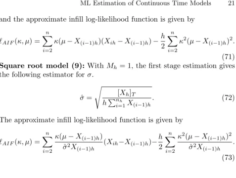
1. Vasicek model (6):Since there is only one parameter in the diffusion function, one could chooseMh= 1. As a result, the first stage estimation
gives the following estimator forσ, ˆ
σ=
r
[Xh]T
and the approximate infill log-likelihood function is given by `AIF(κ, µ) = n X i=2 κ(µ−X(i−1)h)(Xih−X(i−1)h)− h 2 n X i=2 κ2(µ−X(i−1)h)2. (71) 2. Square root model (9):WithMh= 1, the first stage estimation gives
the following estimator forσ. ˆ σ= s [Xh]T hPnh i=1X(i−1)h . (72)
The approximate infill log-likelihood function is given by
`AIF(κ, µ) = n X i=2 κ(µ−X(i−1)h) ˆ σ2X (i−1)h (Xih−X(i−1)h)− h 2 n X i=2 κ2(µ−X(i−1)h)2 ˆ σ2X (i−1)h . (73)
5 Monte Carlo Simulations
This section reports the results of a Monte Carlo experiment designed to compare the performance of the various ML estimation methods reviewed in the previous sections. In the experiment, the true generating process is assumed to be the CIR model of short term interest rates of the form
dX(t) =κ(µ−X(t))dt+σpX(t)dB(t), (74) where κ = 0.1, µ= 0.1, σ = 0.1. Replications involving 1000 samples, each with 120 monthly observations (ie h = 1/12), are simulated from the true model. The parameter settings are realistic to those in many financial appli-cations and the sample period covers 10 years.
It is well-known thatκis difficult to estimate with accuracy whereas the other two parameters, especiallyσ, are much easier to estimate (Phillips and Yu, 2005a, b) and extensive results are already in the literature. Consequently, we only report estimates ofκin the present Monte Carlo study. In total, we employ six estimation methods, namely, exact ML, the Euler scheme, the Milstein scheme, the Nowman method, the infill method, and the Hermite expansion (withK= 1).
Table 1 reports the means, standard errors, and root mean square errors (RMSEs) for all these cases. The exact ML estimator is calculated for com-parison purposes. Since the other estimators are designed to approach to the exact ML estimator, we also report the means and the standard errors of the differences between the exact ML estimator and the alternative estimators.
Exact and Approximate ML Estimation and Bias Reduced Estimation of κ
True Valueκ= 0.1
Method Exact Euler Milstein Nowman In-fill Hermite Jackk Jackk Ind Inf (m=2) (m=3) Mean .2403 .2419 .2444 .2386 .2419 .2400 .1465 .1845 .1026 Std error .2777 .2867 .2867 .2771 .2867 .2762 .3718 .3023 .2593 RMSE .3112 .3199 .3210 .3098 .3199 .3096 .3747 .3139 .2594 Mean of NA .0016 .0041 -.0017 .0016 -.0003 NA NA NA diff Std error NA .0500 .0453 .0162 .0500 .0043 NA NA NA of diff
Note: A square-root model with κ = 0.1, µ = 0.1, σ = 0.1 is used to simulate 120 monthly observations for each of the 1,000 replications. Various methods are used to estimate κ.
Several conclusions can be drawn from the table (Note the true value of
κ= 0.1). First, the ML estimator ofκis upward biased by more than 140%, consistent with earlier results reported in Phillips and Yu (2005a, b). This result is also consistent with what is known about dynamic bias in local-to-unity discrete time autoregressive models. Second, all the approximation-based ML methods perform very similarly to the exact ML method, and hence, all inherit substantial estimation bias from the exact ML method that these methods seek to imitate. Indeed, compared to the estimation bias in exact ML, the bias that is induced purely by the approximations is almost negligible. Third, relative to the Euler scheme, the Milstein scheme fails to offer any improvements in terms of both mean and variation while Nowman’s method offers slight improvements in terms of variation and root mean squared error (RMSE). In terms of the quality of approximating the exact ML, the method based on the Hermite expansions is a clear winner whenK is as small as 1. Further improvements can be achieved by increasing the value ofK, although such improvements do not help to remove the finite sample bias of the ML procedure.
6 Estimation Bias Reduction Techniques
It has frequently been argued in the continuous time finance literature that ML should be the preferred choice of estimation method. The statistical jus-tification for this choice is the generality of the ML approach and its good asymptotic properties of consistency and efficiency. Moreover, since sample sizes in financial data applications are typically large4, it is often expected
4
Time series samples of weekly data often exceed 500 and sample sizes are very much larger for daily and intradaily data.
that these good asymptotic properties will be realized in finite samples. How-ever, for many financial time series, the asymptotic distribution of the ML estimator often turns out to be a poor approximation to the finite sample distribution, which may be badly biased even when the sample size is large. This is especially the case in the commonly occurring situation of drift param-eter estimation in models where the process is nearly a martingale. From the practical viewpoint, this is an important shortcoming of the ML method. The problem of estimation bias turns out to be of even greater importance in the practical use of econometric estimates in asset and option pricing, where there is nonlinear dependence of the pricing functional on the parameter estimates, as shown in Phillips and Yu (2005a). This nonlinearity seems to exacerbate bias and makes good bias correction more subtle.
In the following sections we describe two different approaches to bias cor-rection. The first of these is a simple procedure based on Quenouille’s (1956) jackknife. To improve the finite sample properties of the ML estimator in continuous time estimation and in option pricing applications, Phillips and Yu (2005a) proposed a general and computationally inexpensive method of bias reduction based on this approach. The second approach is simulation-based and involves the indirect inference estimation idea of Gourieroux et al (1993). Monfort (1996) proposed this method of bias corrected estimation in the context of nonlinear diffusion estimation.
In the context of OU process with a known long-run mean, Yu (2007) derived analytical expressions to approximate the bias of ML estimator of the mean reversion parameter and argued that a nonlinear term in the bias formula is particularly important when the mean reversion parameter is close to zero.
6.1 Jackknife estimation
Quenouille (1956) proposed the jackknife as a solution to finite sample bias problems in parametric estimation contexts such as discrete time autoregres-sions. The method involves the systematic use of subsample estimates. To fix ideas, letNbe the number of observations in the whole sample and decompose the sample into m consecutive subsamples each with` observations, so that
N =m×`. The jackknife estimator of a certain parameter,θ, then utilizes the subsample estimates ofθto assist in the bias reduction process giving the jackknife estimator ˆ θjack= m m−1 ˆ θN − Pm i=1θˆli m2−m, (75)
where ˆθN and ˆθli are the estimates of θ obtained by application of a given
method like the exact ML or approximate ML to the whole sample and the
i’th sub-sample, respectively. Under quite general conditions which ensure that the bias of the estimates (ˆθN,θˆli) can be expanded asymptotically in
a series of increasing powers of N−1, it can be shown that the bias in the jackknife estimate ˆθjackis of order O(N−2) rather thanO(N−1).
The jackknife has several appealing properties. The first advantage is its generality. Unlike other bias reduction methods, such as those based on correc-tions obtained by estimating higher order terms in an asymptotic expansion of the bias, the jackknife technique does not rely (at least explicitly) on the explicit form of an asymptotic expansion. This means that it is applicable in a broad range of model specifications and that it is unnecessary to develop explicit higher order representations of the bias. A second advantage of the jackknife is that this approach to bias reduction can be used with many differ-ent estimation methods, including general methods like the exact ML method whenever it is feasible or approximate ML methods when the exact ML is not feasible. Finally, unlike many other bias correction methods, the jackknife is computationally much cheaper to implement. In fact, the method is not much more time consuming than the initial estimation itself. A drawback with jack-knife is that it cannot completely remove the bias as it is only designed to decrease the order of magnitude of the bias.
Table 1 reports the results of the jackknife method applied withm= 2,3 based on the same experimental design above. It is clear that the jackknife makes substantial reductions in the bias but this bias reduction comes with an increase in variance. However, a carefully designed jackknife method can reduce the RMSE.
6.2 Indirect inference estimation
The indirect inference (II) procedure, first introduced by Gouri´eroux, Monfort, and Renault (1993), and independently proposed by Smith (1993) and Gallant and Tauchen (1996), can be understood as a generalization of the simulated method of moments approach of Duffie and Singleton (1993). It has been found to be a highly useful procedure when the moments and the likelihood function of the true model are difficult to deal with, but the true model is amenable to data simulation. Since many continuous time models are easy to simulate but present difficulties in the analytic derivation of moment functions and likelihood, the indirect inference procedure has some convenient advantages in working with continuous time models in finance. A carefully designed indirect inference estimator can also have good small sample properties, as shown by Gouri´eroux, et al (2000) in the time series context and by Gouri´eroux, Phillips and Yu (2007) in the panel context. The method therefore offers some interesting opportunities for bias correction and the improvement of finite sample properties in continuous time estimation.
Without loss of generality, we focus on the OU process. Suppose we need to estimate the parameterκin the model
dX(t) =κ(µ−X(t))dt+σ dB(t). (76) from observations x ={Xh,· · ·, XN h}. An initial estimator of κcan be
ˆ
κN). Such an estimator is inconsistent (due to the discretization error) and
may be seriously biased (due to the poor finite sample property of ML in the lowκor near-unit-root case).
The indirect inference method makes use of simulations to remove the dis-cretization bias. It also makes use of simulations to calibrate the bias function and hence requires neither the explicit form of the bias, nor the bias expansion. This advantage seems important when the computation of the bias expression is analytically involved, and it becomes vital when the bias and the first term of the bias asymptotic expansions are too difficult to compute explicitly.
The idea of indirect inference here is as follows. Given a parameter choice
κ, we apply the Euler scheme with a much smaller step size than h (say
δ=h/10), which leads to ˜ Xtk+δ =κ(µ−X˜tk)h+ ˜Xtk+σ√δt+δ, (77) where t= 0, δ,· · ·, h(= 10δ) | {z } , h+δ,· · ·,2h(= 20δ) | {z } ,2h+δ,· · ·, N h. (78) This sequence may be regarded as a nearly exact simulation from the contin-uous time OU model for small δ. We then choose every (h/δ)th observation
to form the sequence of {X˜k
ih}Ni=1, which can be regarded as data simulated
directly from the OU model with the (observationally relevant) step sizeh. Let ˜xk(κ) ={X˜k
h,· · ·,X˜N hk }be data simulated from the true model, where k = 1,· · ·, K with K being the number of simulated paths. It should be emphasized that it is important to choose the number of observations in ˜xk(κ) to be the same as the number of observations in the observed sequencexfor the purpose of the bias calibration. Another estimator ofκcan be obtained by applying the Euler scheme to{Xhk,· · ·, XN hk }(call it ˜κkN). Such an estimator and hence the expected value of them across simulated paths is naturally dependent on the given parameter choiceκ.
The central idea in II estimation is to match the parameter obtained from the actual data with that obtained from the simulated data. In particular, the II estimator ofκis defined as ˆ κIIN,K= argminκkκˆN − 1 K K X h=1 ˜ κkN(κ)k, (79)
where k · k is some finite dimensional distance metric. In the case where K
tends to infinity, the II estimator is the solution of the limiting extremum problem
ˆ
κIIN = argminκkˆκN −E(˜κkN(κ))k. (80)
This limiting extremum problem involves the so-called binding function
which is a finite sample functional relating the bias to κ.In the case where
bN is invertible, the indirect inference estimator is given by
ˆ
κIIN =b−N1(ˆκN). (82)
The II estimation procedure essentially builds in a small-sample bias correc-tion to parameter estimacorrec-tion, with the bias (in the base estimate, like ML) being computed directly by simulation.
Indirect inference has several advantages for estimating continuous time models. First, it overcomes the inconsistency problem that is common in many approximate ML methods. Second, the indirect inference technique calibrates the bias function via simulation and hence does not require, just like the jack-knife method, an explicit form for the bias function or its expansion. Con-sequently, the method is applicable in a broad range of model specifications. Thirdly, indirect inference can be used with many different estimation meth-ods, including the exact ML method or approximate ML methmeth-ods, and in doing so will inherit the good asymptotic properties of these base estimators. For instance, it is well known that the Euler scheme offers an estimator which has very small dispersion relative to many consistent estimators and indirect inference applied to it should preserve its good dispersion characteristic while at the same time achieving substantial bias reductions. Accordingly, we expect indirect inference to perform very well in practice and in simulations on the basis of criteria such as RMSE, which take into account central tendency and variation. A drawback with indirect inference is that it is a simulation-based method and can be computationally expensive. However, with the continuing explosive growth in computing power, such a drawback is obviously of less concern
Indirect inference is closely related to median unbiased estimation (MUE) originally proposed by Andrews (1993) in the context of AR models and sub-sequently applied by Phillips and Yu (2005a) to reduce bias in the mean reversion estimation in the CIR model. While indirect inference uses expecta-tion as the binding funcexpecta-tion, MUE uses the median as the binding funcexpecta-tion. Both methods are simulation-based.
Table 1 reports the results of the indirect inference method withK= 1000 based on the same experiment discussed earlier. Clearly, indirect inference is very successful in removing bias and the bias reduction is achieved without increasing the variance. As a result, the RMSE is greatly reduced.
7 Multivariate Continuous Time Models
Multivariate systems of stochastic differential equations may be treated in essentially the same manner as univariate models such as (1) and meth-ods such as Euler-approximation-based ML methmeth-ods and transition density-approximation-based ML methods continue to be applicable. The literature
on such extensions is smaller, however, and there are more and more financial data applications of multivariate systems at present; see, for example, Ghy-sels et al (1996) and Shephard (2005) for reviews of the stochastic volatility literature and Dai and Singleton (2002) for a review of the term structure literature.
One field where the literature on multivariate continuous time economet-rics is well developed is macroeconomic modeling of aggregative behavior. These models have been found to provide a convenient mechanism for em-bodying economic ideas of cyclical growth, market disequilibrium and dynamic adjustment mechanisms. The models are often constructed so that they are stochastic analogues (in terms of systems of stochastic differential equations) of the differential equations that are used to develop the models in economic theory. The Bergstrom (1966) approximation, discussed in Section 3.1 above, was developed specifically to deal with such multiple equation systems of stochastic equations. Also, the exact discrete time model corresponding to a system of linear diffusions, extending the Vasicek model in Section 2.1, was developed in Phillips (1972, 1974) as the basis for consistent and efficient es-timation of structural systems of linear diffusion equations using nonlinear systems estimation and Gaussian ML estimation.
One notable characteristic of such continuous time systems of equations is that there are many across-equation parameter restrictions. These restrictions are typically induced by the manner in which the underlying economic the-ory (for example, the thethe-ory of production involving a parametric production function) affects the formulation of other equations in the model, so that the parameters of one relation (the production relation) become manifest else-where in the model (such as wage and price determination, because of the effect of labor productivity on wages). The presence of these across-equation restrictions indicates that there are great advantages to the use of systems procedures, including ML estimation, in the statistical treatment of systems of stochastic differential equations.
While many of the statistical issues already addressed in the treatment of univariate diffusions apply in systems of equations, some new issues do arise. A primary complication is that of aliasing, which in systems of equations leads to an identification problem when a continuous system in estimated by a sequence of discrete observations at sampling intervalh.The manifestation of this problem is evident in a system of linear diffusions for an n−vector processX(t) of the form
dX(t) =A(θ2)X(t)dt+Σ(θ2)dW(t), (83)
whereA=A(θ) is ann×ncoefficient matrix whose elements are dependent on the parameter vector θ1, Σ = Σ(θ2) is a matrix of diffusion coefficients
dependent on the parameter vectorθ2,andW(t) isn−vector standard
Brow-nian motion. The exact discrete model corresponding to this system has the form
Xih=ehA(θ2)Xih+N 0, Z h 0 esA(θ2)Σ(θ 2)esA(θ2) 0 ds ! , (84)
and the coefficient matrix in this discrete time model involves the matrix exponential functionehA(θ2).However, there are in general, an infinite number
of solutions (A) to the matrix exponential equation
ehA=B0 (85)
whereB0=ehA0 =ehA(θ02) andθ0
2is the true value ofθ2.In fact, the solutions
of the matrix equation (85) all have the form
A=A0+T QT−1, (86)
where T is a matrix that diagonalizes A0 (so thatT−1AT = diag(λ
1, ..., λn),
assuming thatA0 has distinct characteristics roots{λ
i :i= 1, ..., n}), Qis a
matrix of the form
Q= 2πi h 0 0 0 0P 0 0 0 −P , (87)
andP is a diagonal matrix with integers on the diagonal. The multiple solu-tions of (85) effectively correspond to aliases ofA0.
Fortunately, in this simple system the aliasing problem is not consequential because there are enough restrictions on the form of the system to ensure identifiability. The problem was originally considered in Phillips (1973). In particular, the coefficient matrix A = A(θ) is real and is further restricted by its dependence on the parameter vector θ. Also, the covariance matrix of the error process R0hesA(θ2)Σ(θ
2)esA(θ2)
0
ds in the discrete system is real and necessarily positive semi-definite. These restrictions suffice to ensure the identifiability of A0 in (85), removing the aliasing problem. Discussion and resolution of these issues is given in Phillips (1973) and Hansen and Sargent (1984). Of course, further restrictions may be needed to ensure that θ1 and
θ2 are identified inA θ01 andΣ θ0 2 .
A second complication that arises in the statistical treatment of systems of stochastic differential equations is that higher order systems involve ex-act discrete systems of the vector autoregressive and moving average type, which have more complicated likelihood functions. A third complication is that the discrete data often involves both stock and flow variables, so that some variables are instantaneously observed (like interest rates) while other variables (like consumption expenditure) are observed as flows (or integrals) over the sampling interval. Derivation of the exact discrete model and the like-lihood function in such cases presents further difficulties - see Phillips (1978) and Bergstrom (1984) - and involves complicated submatrix formulations of matrix exponential series. Most of these computational difficulties have now been resolved and Gaussian ML methods have been regularly used in applied research with these continuous time macroeconometric systems. Bergstrom
(1996) provides a survey of the subject area and much of the empirical work. A more recent discussion is contained in Bergstrom and Nowman (2006).
8 Conclusions
Research on ML estimation of continuous time systems has been ongoing in the econometric and statistical literatures for more than three decades. But the subject has received its greatest attention in the last decade, as researchers in empirical finance have sought to use these models in practical applications of importance in the financial industry. Among the more significant of these applications have been the analysis of the term structure of interest rates and the pricing of options and other financial derivatives which depend on parameters that occur in the dynamic equations of motion of variables that are most relevant for financial asset prices, such as interest rates. The equations of motion of such variables are typically formulated in terms of stochastic differential equations and so the econometric estimation of such equations has become of critical importance in these applications. We can expect the need for these methods and for improvements in the statistical machinery that is available to practitioners to grow further as the financial industry continues to expand and data sets become richer. The field is therefore of growing importance for both theorists and practitioners.
References
1. Ahn, D. and B. Gao, (1999), A parametric nonlinear model of term structure dynamics. Review of Financial Studies, 12, 721–762.
2. A¨ıt-Sahalia, Y., (1999), Transition Densities for Interest Rate and Other Non-linear Diffusions, Journal of Finance, 54, 1361–1395.
3. A¨ıt-Sahalia, Y., (2002), Maximum likelihood estimation of discretely sampled diffusion: A closed-form approximation approach. Econometrica, 70, 223–262. 4. A¨ıt-Sahalia, Y., (2007), Closed-Form Likelihood Expansions for Multivariate
Diffusions. Annals of Statistics, forthcoming.
5. A¨ıt-Sahalia, Y. and R. Kimmel, (2005), Estimating Affine Multifactor Term Structure Models Using Closed-Form Likelihood Expansions. Working Paper, Department of Economics, Princeton University.
6. A¨ıt-Sahalia, Y. and R. Kimmel, (2007), Maximum Likelihood Estimation of Stochastic Volatility Models.Journal of Financial Economics, 83, 413-452. 7. A¨ıt-Sahalia, Y. and J. Yu, (2006), Saddlepoint approximation for
continuous-time Markov Processes. Journal of Econometrics, 134, 507-551.
8. Andrews, D. W. K., 1993, Exactly Median-unbiased Estimation of First Order Autoregressive/unit Root Models, Econometrica, 61, 139–166.
9. Bakshi, G. and N. Ju, (2005), A Refinement to A¨ıt-Sahalia’s, 2002 “Maxi-mum Likelihood Estimation of Discretely Sampled Diffusions: A Closed-Form Approximation Approach”,Journal of Business , 78 (5), 2037-2052.