Cahsai, A., Anagnostopoulos, C. and Triantafillou, P. (2015) Scalable data
quality for big data: the Pythia framework for handling missing values. Big
Data, 3(3), pp. 159-172. (doi:
10.1089/big.2015.0002
)
This is the author’s final accepted version.
There may be differences between this version and the published version.
You are advised to consult the publisher’s version if you wish to cite from
it.
http://eprints.gla.ac.uk/109175/
Deposited on: 20 August 2015
Enlighten – Research publications by members of the University of Glasgow
http://eprints.gla.ac.uk
Scalable Data Quality for Big Data:
The Pythia Framework for Handling Missing Values
A. Cahsai, C. Anagnostopoulos, P. Triantafillou
School of Computing ScienceUniversity of Glasgow, G12 8QQ, Glasgow, UK
[email protected]; [email protected];
[email protected]
ABSTRACT
Solving the missing-value (MV) problem with small estima-tion errors in large-scale data environments is a notoriously resource-demanding task. The most widely used MV im-putation approaches are comim-putationally expensive because they explicitly depend on the volume and the dimension of the data. Moreover, as datasets and their user community continuously grow, the problem can only be exacerbated. In an attempt to deal with such problem, in our previous work [1], we introduced a novel framework coined Pythia, which employs a number of distributed data nodes (cohorts), each of which contains a partition of the original dataset. To perform MV imputation, the Pythia, based on specific ma-chine and statistical learning structures (signatures), selects the most appropriate subset of cohorts to perform locally a Missing Value substitution Algorithm (MVA). This selection relies on the principle that that particular subset of cohorts maintains the most relevant partition of the dataset. In ad-dition to this, as Pythia uses only part of the dataset for imputation and accesses different cohorts in parallel, it im-proves efficiency, scalability and accuracy comparing against a single machine (coined Godzilla), which uses the entire massive dataset to compute imputation requests. Although this paper is an extension to our previous work, we particu-larly investigate the robustness of the Pythia framework and show that the Pythia is independent from any MVA and sig-natures construction algorithms. In order to facilitate our research, we considered two well-known MVAs (namely K-nearest neighbor and expectation-maximization imputation algorithms) as well as two machine and neural computa-tional leaning signature construction algorithms based on adaptive vector quantization and competitive learning. We prove comprehensive experiments to assess the performance of the Pythia against Godzilla and showcase the benefits stemmed from this framework.
Categories and Subject Descriptors: H. Information Systems; I.5.3 Clustering.
Keywords: Big data; Scalability; Missing values;
Impu-.
tation; Adaptive vector quantization; Self organizing maps; Adaptive resonance theory.
1.
INTRODUCTION
Data quality is a major concern in big data processing and knowledge management systems. One relevant problem in data quality is the presence of missing values (MVs). The MV problem should be carefully addressed, otherwise bias might be introduced into the induced knowledge. Common solutions to the MV problem either fill-in the MVs ( impu-tation) or ignore / exclude them. Imputation entails aMV substitution algorithm(MVA) that replaces MVs in a dataset with some plausible values.
On the one hand, most computational intelligence and ma-chine learning (ML) techniques (such as neural networks and support vector machines) fail if one or more inputs contains MVs and thus cannot be used for decision-making purposes [2]. Furthermore, the choice of different MVAs affects the performance of ML techniques that are subsequently used with imputed data [3]. On the other hand, the MV problem abounds: it can be found, for instance, in results from medi-cal experimentation and chemimedi-cal analysis, in datasets from domains such as meteorology and microarray gene monitor-ing technology [6], and in survey databases [7]. MVs can occur e.g., due to wireless sensor faults, not reacting experi-ments, or participants skipping survey questions. Industrial and research databases include MVs [8], e.g., maintenance databases have up to 50% of their entries missing [9]. Pa-tient records in medical databases lack some values; inter-estingly, a database of patients with cystic fibrosis missing more than 60% of its entries was analyzed in [10]. Moreover, gene expression microarray data sets contain MVs, making the need for robust MVAs apparent, since algorithms for gene expression analysis require complete gene array data [11].
Motivations. Given the significance of MVAs, three notes are in order: Firstly, MVAs which can ensure low estimation errors are computationally expensive and typi-cally their performance is largely dependent on dataset sizes and on the data dimension. Secondly, nowadays, datasets can be massive. Even worse, existing datasets grow signifi-cantly with time; it is not surprising that most MVAs in the literature are typically tested over small-to medium sized datasets. Lastly, as if the scalability limitations imposed by dataset sizes were not enough, in many applications the user community (e.g., in shared scientific datasets in data centers accessed by scientists from all over the world) can be very large and thus the MV imputation input arrival rates can
become high as well. These facts pose a scalability night-mare.
The scalability gospel (as established by the seminal work from Google researchers producing the Map-Reduce (MR) [12] data-access paradigm and systems such as the Google File System [13]) rests on the notion ofscaling out: that is, (i) employ a large number of commodity (off-the-shelf and thus inexpensive) machines, each storing a much smaller par-tition of the original dataset, and (ii) access them in parallel. However, MR is not a panacea, for the following rea-sons. First, not all complex problems are ‘embarrassingly parallelizable’ and amenable to MR techniques. In particu-lar, there exist MVAs coming with small imputation errors, which are not MR-able [14]. The MVAs are basically (com-plex) statistical and machine learning algorithms like the ex-pectation maximization imputation algorithm [20] and the sequential multivariate regression imputation [19] algorithm. Such algorithms are based on iterative processes, i.e., the MR scheme needs to process data again and again. In such MVAs, the intermediate processes need to communicate to each other and possibly processing requires lot of data to be shuffled over the network of distributed data nodes. In ad-dition, when the Map phase generates too many keys, then sorting takes for ever. Moreover, it’s not always straight forward to implement any potential ML-based imputation algorithm as a MR program [14]. Further, MR does not ef-ficiently handle streaming MV imputation requests. Since the Map output stream it is not kept into the memory, this will be inefficient especially when dealing with a high rate of MV imputation requests. In the context of MVAs, even if they were ‘embarrassingly parallelizable’, not all parti-tions may be relevant. Specifically, given the fact that a number of machines are involved for locally executing the MVAs, the entire massive dataset is partitioned into smaller datasets distributed onto the machines. This dataset parti-tioning is simple in the sense that each data node contains a unique, non-overlapping subset of the entire dataset. It may very well be the case that a number of the machines hold data that cannot help (or even hurt) in the MV im-putation process. And, obviously, engaging only a fraction of all machines will introduce large benefits: First with re-spect to performance. MV imputation will be shorter, as these times typically depend on the worst performing ma-chine and with increasing mama-chine numbers the probability of a mall-performing machine increases. Further, overall MV imputation throughput will be higher, as each imputation will be taxing fewer overall system resources (processors, communication bandwidth and disks). Second, with respect to MV estimation errors. In fact, as we shall formally show later, engaging all machines and their dataset partitions may actually introduce large additional MV estimation errors.
Goals. In this work, we will consider a stream of MV imputation requests, hereinafter referred to as inputs. An input is a multi-dimensional vector with some MVs in cer-tain dimensions, arriving at a data system. Typically, the system is presented with a batch of data items with MVs, which must be added to the system after MVs have been estimated. It is worth noting in this case that, in order to trace back imputed MVs in the system, eachimputed in-put is accompanied with an imin-putation meta-data vector containing the dimension index of each estimated/imputed value. Through this meta-data flagging technique, the sys-tem makes clear what values arerealvalues orimputedones.
From a data management viewpoint, this enables the system to ensure that the stored data maintain integrity by clearly flagging MVs as an important operation and legal matter.
There are two system alternatives to impute the MVs. The first is based on employing a single machine which stores the whole of the dataset. We affectionately call this ma-chine Godzilla. Godzilla can employ any MVA to perform the MV imputations. As motivated earlier, this approach suffers from several disadvantages. The second alternative employs a (potentially large) number of machines, referred to ascohorts, each storing a partition of Godzilla’s dataset. Each cohort stores a unique and non-overlapping subset of the massive Godzilla’s dataset. Imputation execution en-gages cohorts in parallel, whereby each cohort runs an MVA on a much smaller local dataset. This can introduce dra-matic performance improvements. As an illustration, let us assume 50 cohorts and an MVA operating on a dataset of sizenwith asymptotic complexityO(n2), orO(n3) [4], [6]. A scale-out execution is expected to speedup input process-ing by a factor of 502 = 2,500 (or 503 = 125,000) as such
MVA runs in parallel on a dataset of size 1
50n. Moreover,
this alternative affords the possibility of accessing only a subset of all cohorts for a given input.
The formidable challenges here entail: (i) for data accu-racy (estimation-error) reasons, we should ensure that the subset of cohorts contacted achieve similar, if not smaller es-timation errors, compared to the errors that Godzilla would yield; (ii)swiftlydetermine cohort to engage per imputation, achieving large efficiency/scalability gains.
2.
BACKGROUND & RELATED WORK
2.1
Missing data
Assume a data set X of d-dimensional data points with some MVs on a certain dimensionXi. Data onXi are said
to bemissing completely at random (MCAR) if the proba-bility of MV onXi,q, is unrelated to the value ofXi itself
or to the values of any other dimensions. If data are MCAR, a reduced sample of X will be a random sub-sample ofX; MCAR assumes that the distributions of MVs and complete data are the same. Data on Xi are said to be missing at
random (MAR) ifqdepends on the observed data, but does not depend on the MV itself. In MAR, the dimension as-sociated with MVs has a relation to other dimensions, i.e., MVs can be estimated by using the complete data of other dimensions. Data onXiaremissing not at random(MNAR)
ifq depends on the MVs and, thus, imputation is not per-missible in this case.
2.2
Related work
Missing data hinder the application of many statistical analysis and ML techniques available in off-the-shelf soft-ware. To analyze X with MVs, certain MVAs have been proposed [15]. The simplest method is discarding the data points with MVs or removing the corresponding dimensions. Both removals of such points and dimensions result in de-creasing the information content of X and are applicable only when (i) X contains a small amount of MVs, and (ii) the analysis of the remaining complete points will not be biased by the removal. There are many MVAs varying from na¨ıve methods, e.g., mean imputation, to some more robust methods based on relationships among dimensions. In the
value. Themean / mode imputation replaces MVs of a di-mension by the sample mean / mode of all observed values of that dimension. Inhot deck MVA [16], a MV is filled in with a value from an estimated distribution w.r.t. X. In the K-nearest neighbors MVA [17], the MVs of a point are imputed considering the K most similar (observed) points fromX. The regression- and likelihood-based MVAs are in-troduced in [18]. In regression-based imputation [19], the MVs of a point are estimated by regression of the dimen-sions corresponding to MVs on the dimendimen-sions associated to the observed values of that point. This approach argues that dimensions have relationships among themselves; if no rela-tionships exist among dimensions inX and the dimensions corresponding to MVs, such MVA will not be precise for im-putation. Likelihood-based imputation [18] is based on pa-rameter estimation in the presence of MVs, i.e.,X’s param-eters are estimated by maximum likelihood or maximum a posteriori procedures relying on variants of the Expectation-Maximization algorithm. The multiple imputation MVA [20], instead of filling in a single value for each MV, re-places each MV with a set of plausible values that represent the uncertainty about the actual value to impute. These multiply-imputed datasets are then analyzed by using stan-dard procedures for complete data and combining the re-sults from these analyses. In case of MVs in time series, the models in [21] (using dynamic Bayesian networks), [22] (us-ing matrix completion), and [23] (us(us-ing Gaussian mixtures clustering) recover MVs in motion capture sequences, vital signs, and micro-array gene expression streams, respectively. Furthermore, ML-based MVAs, e.g., decision-trees and rule-based methods, generate a model fromX that contain MVs, which is used to perform classification that imputes the MVs (see [3] and the references therein). Finally, the imputation framework [8] applies most existing MVAs (base methods) to improve their accuracy of imputation while preserving the asymptotic computational complexity of the base methods. The interested reader could also refer to [8], [11] and [24] (and the references therein) for a comprehensive survey of the most recent MVAs.
3.
DEFINITION
3.1
Definitions & Notations
Definition 1. Given a setX ofd-dimensional data points,
X = {x1, . . . ,x|X |}, for each xi we define the imputation
meta-data vectorwi = [wik]> withwik = 0 wheneverxi’s
k-th dimensional value is missing; otherwisewik= 1. We
ex-pressxias (zi,zmi ), wherezi∈Rd 0
denotes observed values andzmi ∈R(d−d
0)
denotes MVs, withd0=Pd k=1wik.
Definition 2. Given a finite integerm >0,Xi is a
parti-tion ofX such thatX ≡ ∪m
i=1Xi andXi6=Xj, i6=j. Si
de-notes the machine (cohort), which maintainsXi, performs a
MVA overXi, and is indexed byi,i= 1, . . . , m. S={Si}mi=1
is the set of all cohorts. The (imaginary)GodzillaS0
assem-bles allXi and is capable of performing a MVA overX.
Definition 3. A single MV input on MVA isi = (x,w) and output is ˆx expressed by (z,ˆzm). ˆx ∈
Rd is referred to asestimate containing ˆzm∈R(d−d
0)
of imputed MVs by MVA. Ifxais the actual vector, the absolute reconstruction
error ise=kxˆ−xak;kxkdenotes the Euclidean norm.
3.2
MVAs in our framework
As our approach is independent of any particular MVA, we overview and experiment with two popular and repre-sentative MVAs in our framework. Note, in our previous work we also experiment with the REG [19] MVA algorithm. To exemplify our framework and methods, we employ the weighted K-nearest neighbors (KNN) [17] and Expectation Maximization imputation method (EM) [20]. These MVAs are widely used for multivariate imputation in many scien-tific areas.
3.2.1
Weighted
K-nearest neighbors imputation
KNN is widely used [24] since it has many attractive char-acteristics: it is a non-parametric method, which does not require the creation of a predictive model for each dimension with MV and takes into account the correlation structure of the data. KNN is based on the assumption that points close in distance are potentially similar. For given input (xi,wi)
with xi = (zi,zmi ), KNN calculates a weighted Euclidean
distanceDij betweenxiandxj∈ X such that
Dij= Pd k=1wikwjk(xik−xjk) 2 Pd k=1wikwjk !1/2 .
The MV of the k-th dimension of xi (i.e., zmik of z
m
i ) is
estimated by the weighted average of non-MVs of the K most similarxj toxi, i.e., ˆzmik =
PK j=1 D−ij1 PK v=1D −1 iv xjk. KNN
is typically used with K=10,15,20; theses values have been favored in previous studies [24], [25]. (In our experiments we will use K=10).
Remark 1. A naive approach for searching the closestd -dimensional data point with respect to a given pointxover a dataset of size n = |X | requires O(nd) time. This im-plies also O(ndK) time for retrieving the K nearest data points. Nonetheless, we could built a d-dimensional tree over the points ofX to allow to efficiently performK near-est neighbors search. Such structure is ‘good’ for searches in low-dimensional spaces. However, its efficiency decreases as dimensionality grows, and in high-dimensional spaces this structure gives no performance over naive O(ndK) linear search. Overall, the KNN imputation algorithm can build a d-dimensional tree with O(nlogn) time complexity and achieves imputation time complexity close toO(Kdlogn).
3.2.2
Expectation Maximization imputation
The EM algorithm is an iterative algorithm for estimating MVs by maximizing the likelihood function [18]. Assume thatXis generated by a probability density functionf(X |θ), whereθis a parameter of the model. The likelihood function
L(θ|X) is a function of the parameterθ for fixed X. For mathematical convenience, likelihood function is represented by its log-likelihood functionl(θ|X) = ln(L(θ|X)). Without loss of generality, consider for fixed X a set of parameters
θ ={θ1, . . . , θt} witht >0. For every θi∈θ, we calculate
l(θi≤t|X). The obtained outcome shows that how likelyX
is observed under θi. The highest the outcome is the most
likely X is observed under that parameter. In general, L
is used to identify the value of θ, which is best supported by X. For a set X, which contains observed values, Xobs
and MVsXmiss, the log maximum likelihood ofX isl(θ|X)
= l(θ|Xobs,Xmiss) = l(θ|Xobs) + lnf(Xmiss|Xobs, θ). The
estimation (MLE) ofθ froml(θ|Xobs) in order to maximize
the MLE ofl(θ|X). The EM algorithm consists four steps: Step (i) replace MVs by estimated values, Step (ii) estimate
θ (also known as E-step), Step (iii) re-estimate MVs using the new θ (referred as M-step ), Step (iv) re-estimate θ, iterate until convergence [18].
To illustrate how the EM algorithm is used for imputation, consider the d-dimensional mean vector u = [u1, . . . , ud]>
and covariance matrix Σ = [σjk] withj, k= 1, . . . , d. Both
uand Σ refer to learning parameterθ, i.e.,θ= (u,Σ). Ini-tially,µand Σ are calculated considering only the non miss-ing values, i.e., from theXobsset. Then, the EM imputation
algorithm calculates each step as follows:
• Step 1: For eachxi∈ X, ifwik= 0 then we estimate
ˆ
zm
ik =uk. Note thatwi remains unchanged in order
to help us identify which dimensions are observed or missed in the original data setX.
• Step 2: Estimation of parameterθt at iterationt≥1.
For eachk, j= 1, . . . , dwe calculate:
E |X | X i=1 xik|Xobs, θt = |X | X i=1 xtik and E |X | X i=1 xikxij|Xobs, θt = |X | X i=1 xtikxtij+ctjki with ˆ zikm= ( xik, ifwik= 1 E Pn i=1xik|Xobs, θt ifwik= 0 and ctjki= ( 0, ifwik= 1 orwij= 1 xikxij|Xobs, θt ifwik= 0 andwij= 0
At the end of this step, the purpose is to estimate the sufficient statistics, i.e., mean, variance, and covari-ance so that the following step can update the param-eterθt. Specifically, this step estimatesuand Σ, and
uses them to build a set of regression equations that predict the missing values from theXmissset. This is
achieved by thesweepregression operator [18] realizing the conditional expectations. Such operator combines the mean vector and the covariance matrix into a single augmented matrix and applies a series of transforma-tions that produce the desired regression coefficients and residual variances.
• Step 3: re-estimate MVs using the new θt parameter.
This step becomes a straightforward estimation prob-lem that uses the filled-in sufficient statistics from the previous step to impute the missing values. Then, for eachk, j= 1, . . . , dwe calculate: u(kt+1)= (|X | −1)−1 |X | X i=1 ˆ zikm and σjk(t+1)= (|X | −1)−1 |X | X i=1 [(xij−µj)(xik−µk) +cjki]
• Step 4: If |l(θt+1|X)−l(θt|X)| ≤ then terminate
(converge); otherwise, go to Step 2. We set= 10−3 for convergence.
Remark 2. Each iteration takesO(nd) computations given that n = |X |. However, the termination behavior of EM is not easy and guaranteed. Theoretically speaking, with-out any stopping threshold (or, setting a stopping threshold
= 0), EM would infinitely converge up to an infinite pre-cision, i.e., = 0. Hence, the theoretical runtime of EM is infinite. Any small and non-negative threshold > 0 and
→0 forces EM to terminate earlier. But it will be hard to get a theoretical limit here different thanO(ndt) where
tis the number of iterations up to achieving precision close
to.
4.
THE PYTHIA FRAMEWORK
The Pythia framework in [1] employs a potentially large number of cohorts,S. Each cohort,Si∈ S, stores a unique
and non-overlapping subset of a massive datasetX. Impu-tation execution engages cohorts in parallel, whereby each cohort runs a MVA on a much smaller local dataset,Xi.
Ac-cordingly, for some input, Pythia must swiftly predict the appropriate cohort or cohorts,S0, in which the MVA is going to be executed. Pythia predictsS0⊆ S
for each input based on per-cohort signatures [1]. Each cohort Si constructs a
signature Pi from Xi. Pi reflects the current structure of
data points inXi. The idea behind a signature is thatSi is
engaged for a givenioncexcan be ‘explained’ throughPi.
Si provides its (locally) createdPi to Pythia, which stores
all signatures forming P = {Pi}mi=1. The operation of the
Pythia framework is as follows: Given in imputation request (input)i,
• Step 1: Pythia predicts the subset of cohorts S0 ⊆ S
with respect toP
• Step 2: Pythia engages only the cohorts fromS0 send-ing the inputito them.
• Step 3: Each cohortSi∈ S0
– Step 3.1: Siinvokes locally a MVA and
– Step 3.2: Suprovides its estimate ˆxi to Pythia.
• Step 4: Pythia constructs the aggregate estimate ˆx
that is sent to the cohorts fromS0.
• Step 5: EachSi∈ S0can exploit ˆxfor updating itsPi.
• Step 6: Pythia uses ˆx for updating the signatures set
P.
• Step 7: Pythia stores the imputation meta-data vector
wto trace back imputed MVs in the system.
4.1
Signatures
The general idea of a signaturePi is to represent
knowl-edge on the probability density function (or distribution) of the Xi of a cohort. ThroughPi we optimally quantize the
Xispace of each cohortSito estimate the distribution of the
underlyingXi. Through adaptive vector quantization, which
is achieved by unsupervised competitive learning, we obtain a set of ‘representatives’ overXi. The information conveyed
representatives drives the decision on whether a cohortSi
is eligible for being engaged in a given imputation requesti. In this section, we propose two methods for signatures cre-ation based on two adaptive vector quantizcre-ation algorithms, namely the Adaptive Resonance Theory [26] and the Self Organizing Maps [5].
4.1.1
Adaptive Resonance Theory Signature
Each cohortSi ∈ S employs the ART [26], an
unsuper-vised learning model from the competitive learning paradigm, in order to locally constructPioverXi. In ART, whose
al-gorithm is shown in Alal-gorithm 1, eachxk∈ Xiis processed
by finding the nearest representative c∗ ∈ Rd to xk, i.e.,
c∗= arg minc∈Cikc−xkk, whereCiis the set of represen-tatives. Then, it is allowedxk to modify/updatec∗ only if
c∗is sufficiently close toxk(c∗is said to ‘resonate’ withxk)
i.e., ifkc∗−xkk≤ρifor somevigilance ρi>0. In this case,
c∗is updated through the rulec∗←c∗+ηi(xk−c∗), where
ηi∈(0,1) is a learning rate, which gradually decreases.
Oth-erwise, i.e.,kc∗−xkk> ρi, a new representativecis formed
handlingxksuch thatc=xk andCi← Ci∪ {c}.
Definition 4. The ART signaturePiof cohortSioverXi
is the triple
Pi=hCi, ρi, ηii. (1)
ALGORITHM 1: ART signature creation algorithm at cohortSi Input: Xi, ηi, ρi Output: Ci Ci={x1}; for1< k≤ |Xi|do b∗=kc∗−xkk= minc∈Ci kc−xkk; if b∗> ρithen Ci← Ci∪ {xk}; else c∗←c∗+ηi(xk−c∗); end end
Definition 5. We say thatx is amember of an ART Pi
signature, notated by x ∈ Pi, iff minc∈Ci k c−x k≤ ρi;
otherwise,x6∈Pi.
The statement ‘x∈Pi’ denotes that there is at least one
c∈ Cisuch thatxis placed close tocwith distance less than
ρi, for instance, the closest representativec∗tox. The more
representativesc∈ Cisatisfy the criterionkc−xk≤ρi, the
more appropriateCi is forx. In this sense, if x∈ Pi then
x can be represented by at least one representative from
Xi. Based on this intuition, ifx∈Pi, cohortSi provides a
rather good estimate for some missing parts ofxcompared to a cohortSj associated with aPjfor which it holds true
thatx6∈Pj. The latter case indicates that no representative
fromCjcan be a representative point forx.
Sinceρirepresents a threshold of similarity between points
and representatives, thus, guiding the ART algorithm in de-termining when a new representative should be formed, it should depend onXi. In order to give a physical meaning to
ρi, it is expressed through a set of percentagesαk ∈ (0,1)
of the ranges between the lowestxmin
k and highestxmaxk
val-ues of each dimension k of points inXi, k= 1, . . . , d. Let
ri = [(xmax1 −x1min), . . . ,(xmaxd −x
min
d )]
>
and the diagonal
d×dmatrixAwithA[k, k] =αk. Thenρi=kArik. High
αkvalues result to a low number of representatives and vice
versa. EachSidetermines aρioverXi, createsPithrough
Algorithm 1, and sendsPito Pythia.
Remark 3. When dealing with mixed-type data points, e.g., consisting of categorical, binary, and continuous at-tributes, we can adopt appropriate distance metrics [29] for the distance between xk and xl instead of using the
Eu-clidean distancekxk−xlk; this does not spoil the generality
of signature creation.
4.1.2
Self-Organizing Map Signature
The basic SOM [5], whose algorithm is shown in Algo-rithm 2, is formally a nonlinear, ordered, smooth mapping of high dimensional vectorial data manifolds, input vector (x), onto the vectorial elements (representatives) of a reg-ular, low dimensional lattice L. SOM implicitly captures the structure of x and, in particular, identifies the repre-sentatives of x that have similar statistical characteristics in the high-dimensional vector space. The most important characteristic of the SOM is the capability of producing a structuredorderingof the vectors, i.e., similar vectors in the input space are mapped to neighboring representatives of the map. The incrementally formated representatives estimate the distribution of a datasetX.
Consider the vectorsx1, . . . ,x|Xi| from the datasetXi of
cohort Si. The on-line SOM algorithm maps incrementally
these vectors into a latticeLcomposed of`i×`i
represen-tatives, `i > 0, i.e., the number of representatives in Si
is `2
i. Hereinafter the parameter ` is referred to as
lat-tice width. The representatives are linked together by a neighborhood relationshiph(j, j0) over the indiciesj, j0∈ L,
j, j0= 1, . . . , `2
i. With each representative onL, we associate
a representativecjof latticeLwith the same dimension asx.
The`2i representatives ofLare initialized randomly among
the input vectors. By assuming a general distance metric betweenxandcj,D(x,cj), the image ofxonto the lattice
Lis defined by the winning representativec∗j that matches
best withx, i.e.,
j∗= arg min
j∈LD(x,cj). (2)
In the Euclidean space whereD(x,cj) =kx−cjk2, i.e.,
the 2-norm, the on-line SOM algorithm, at thekthinputxk,
k= 1, . . . ,|Xi|, consists of two steps:
• Step 1: (Assignment) Vectorxk is assigned to a
win-ning representative c∗j, i.e., k xk−c∗j k= minj∈L k
xk−cjk
• Step 2: (Update) All representatives inLare updated as
cj=cj+η(k)h(j, j
∗
;k) (xk−cj). (3)
The parameterη(k) ∈ (0,1) called learning rate is a non-increasing function ofk. A good choice ofη(k) im-proves significantly the convergence of SOM [5]; usu-ally η(k) = 1+η(ηk(−k−1)1) with η(0) = 1. A discussion
aboutη(k) and the choice of an ‘optimal’ learning rate can be found in [5]. The h(j, j∗;k) is a smoothing Kernel function defined over indiciesj, j∗∈ L, usually given by the Gaussian neighborhood function:
h(j, j∗;k) = exp −krj−r ∗ j k2 2β2(k) .
Vectors rj and r∗j are, respectively, the locations of
representativescjandc∗jonL. The topological
neigh-borhood is symmetric around the winning representa-tive, which has the maximum value. Parameter β(k) is the width of the neighborhood with initial valueβ0
defined as β(k) = β0exp(−Tk
β), where Tβ is a con-stant. The boundaries of neighborhood h(j, j∗;k) de-pends on β(k). A small width value corresponds to narrow boundaries, while with high width, the bound-aries contains more neighbors.
Remark 4. Since the size of|Xi|= m1|X | is significantly
large thus we can assume that the on-line algorithm of SOM converges. However, if the algorithm has not converged then an additional iteration (or, iterations) is performed until a termination criterion holds true. This criterion, which is compared to a percentage convergence threshold > 0, refers to the 1-norm between successive estimates of the rep-resentatives, i.e., the algorithm converges ifP
j∈Lkwj(k)−
wj(k−1)k1< ·Pj∈Lkwj(k−1)k1withkwjk1=Pdi|wji|
andk >0.
LetCibe the set of representatives {cj} `2
i
j=1belonging to
latticeL.
Definition 6. The SOM signaturePiof cohortSioverXi
is the tuple
Pi=hCi, `ii. (4)
Each cohort Si ∈ S can locally set the number of
repre-sentatives `2i in its lattice thus giving it the flexibility to,
independently of the other cohorts, determine the ‘resolu-tion’ (quality) of data space quantization. Evidently, the higher the value of`ithe more fine grained the resolution of
Xiquantization gets; however at the expense of higher space
requirements. On the other hand, a low value of`i might
not be enough to represent the diversity of the data inXi.
The distance betweenxand its winner representativecj∗ plays a significant role on determining how appropriately
x is represented by Pi. The fact that cj∗ is the closest representative to x does not covey any information about how qualitatively the topologically close data space area of
cj∗ represents the topologically close data space are tox. Given a smooth distance metric betweenxandcj∗we define asdegree of membership ofx toPi the functionµi :Rd → [0,1] such that
µi(x) = exp(− kx−cj∗k22). (5) Aµi value close to unity indicates thatxis topologically
very close to its winning representativecj∗thusxis believed to be a member ofPi with a high degree. Aµi value close
to zero indicates thatxis topologically very distant from its winning representative cj∗. Hence, in this case x is not a member ofPi.
Definition 7. We say that x is a member of a SOMPi,
notated byx∈µPi, with a degree ofµi(x)> ,→0.
ALGORITHM 2: SOM signature creation algorithm at cohortSi Input: Xi,`i,β0,Tβ Output: Ci Initialize cj,j∈ L; Ci={c1, . . . ,c`2 i}; for(1≤k≤ |Xi|)do j∗= arg minj∈Lkxk−cjk2; cj←cj+η(k)h(j, j∗;k)(xk−cj),j∈ L; end
Remark 5. Once Pythia has produced the estimate ˆxgiven an inputi = ((z,zˆm),w), it updates locally the signatures of those cohorts which were engaged in the imputation pro-cess. In case of ART signatures, the reader could refer to [1] which reports on the expected magnitude of change of the representatives in an ART signature due to the estimate. In the case of SOM signatures, the updates are the same with that of the ART signature, provided that the winner repre-sentative cj∗ of input zget updated with a small constant rateη; the same rate is adopted in ART signatures.
4.2
Cohorts prediction
Up to this point, we have shown how to use signatures as a guiding light to select appropriate cohorts for MV im-putations. Now, our concern is twofold: MV imputations must be (i) low cost and (ii) high accuracy. Low cost (once signature processing is performed) refers to the communi-cation cost between Pythia and cohorts and to the cost of running MVAs at cohorts. High accuracy refers to low RMSE. Therefore, in our previous work we presented algo-rithms with these in mind. Now, we further propose two cohorts prediction algorithms corresponding to ART- and SOM-signatures, which engage the top-Krelevant cohorts for an imputation request, 1≤ K ≤m. Under this class of algorithms, Pythia is not involved in producing the (final) estimate ˆx, instead, only the top-Kbest cohorts are engaged for doing this locally. Pythia communicates only with these cohorts, which run the MVA in parallel, thus, this optimizes our cost metric. Note, the reader could refer also to the accuracy-aware class of algorithms in our previous work [1], in which Pythia is (merely) engaged in the final estimate.
4.2.1
ART signature cohort prediction
For simplicity consider the top-1 (best cohort) scheme, i.e., K= 1. Given imputation request i and a set of ART signatures, Pythia determines the best cohort S∗∈ S with
P∗=hC∗
, ρ∗, η∗isuch that the following criteria hold true:
• Criterion C1: c∗ = arg minc∈∪m
i=1Ci k c−z k and
c∗= arg minc∈C∗kc−zk, i.e.,c∗∈ C∗is the closest representative tozamong all representatives from all signatures, and
• Criterion C2: z∈P∗, i.e., the vectorz is member of the ART signatureP∗.
Note thatz∈Rd 0
with 0< d0 =Pd
k=1wk < dprovided
Pythia calculatesρ∗(d0) ≤ρ∗
associated with then dimen-sions ofq∗corresponding to thennon-MVs. Then, it checks ifkc∗−zk≤ρ∗(d0) dealing only with thed0 dimensions of
c∗. Pythia engages only the best cohortS∗, which produces the final ˆx. If there is no cohort that satisfies criteria C1 and C2, then Pythia engages the cohort that satisfies only criterion C1. If K > 1 one can repeat the above criteria for the topKcohorts ranked with the distance between the correspondingc∗j and z, 1≤j ≤ K< m. In this case the
final ˆxis produced by aggregating all ˆxjwith 1≤j≤ K.
4.2.2
SOM signature cohort prediction
Consider again for simplicity the top-1 (best cohort) scheme. Given imputation request i and a set of SOM signatures, Pythia determines the best cohortS∗∈ S as follows:
• Step 1: Find the winner prototypec∗i = arg minc∈Cik
z−ckfrom signatureSi,∀i.
• Step 2: Define a membership indicator Ii(z) = 1 if
µi(z)> ; otherwise 0,∀i.
• Step 3: Calculate the normalized membership degree ˜
µi(z) =
µi(z)Ii(z)
Pm
k=1µk(z)Ik(z)
and select the cohort with the maximum value of ˜µ. If for all cohorts Si ∈ S, it holds true that Ii(z) = 0,
i.e., z cannot be represented by any winner representative from all signatures, then Pythia engages the cohort whose winner representative is the closest to input z among all winner representatives (from all signatures). IfK>1, then Pythia engages (at most) the top K cohorts ranked with respect to the ˜µvalue. In this case the final ˆxis produced by aggregating all ˆxjwith 1≤j≤ K.
4.3
Pythia asymptotic complexity
Letξ be the average number of representatives per ART signature. In a SOM signature we have`2 representatives, assuming that the latices from all signatures have the same number of representatives. For the top-Kclass of algorithms for cohorts prediction, we adopt ad-dimensional tree struc-ture over all representatives from all ART and SOM signa-tures inP. Given imputation input i, Pythia performs a 1NN search withO(dlog(mξ)) andO(dlog(m`)) time since it searches over all representatives in ART and SOM sig-natures, respectively, from all signatures∪m
i=1Ci given that
K= 1. Pythia requiresO(mdξ) andO(md`2) space, respec-tively, for ART and SOM signatures. Pythia requiresO(K) communication with cohorts fromS.
4.4
Limitation of the Signatures Algorithms
The main limitations of the ART- and SOM-based sig-natures algorithms are the nature of their parameters that need to be defined in advance. In the SOM algorithm, a fixed number of representatives in the latticeLmust be de-termined beforehand. In this context, a good choice of the lattice size (number of representatives`2) has a significant
impact on the overall quality of the derived self-organized clusters. A small`value, i.e., a low number of representa-tives, might not be sufficient enough to represent the topo-logical structure of the data, thus capturing their statistical characteristics. On the other hand, a huge number of rep-resentatives scatter similar data items into more than one
clusters. In addition, this comes with a significant number of ‘training’ samples for the SOM algorithm to converge. Likewise, a good choice of the vigilance parameter ρplays an important role on incremental data space partitioning in the ART algorithm. A relatively high vigilance value produces few clusters/representatives, in which ‘non-similar’ data points are grouped together. On the other hand, a small vigilance value yields the formation of a high number of representatives that might contain few data points and in-crease the signature size, i.e., the representatives setC, per cohort. An appropriate determination of the vigilanceρand the lattice size`highly depends on the statistical properties of the underlying data in each cohort, individually. That is a ‘good’ vigilance or lattice size for one cohort might not be suitable for another one. Therefore, a fine tuning of these parameters is essential in order to get optimal quality of data space partitioning. The reader could also refer to for a discussion on good values for vigilance [27] and lattice size [28] corresponding to the ART and SOM algorithms, respec-tively.
5.
PERFORMANCE EVALUATION
5.1
Experimental Setup
We conducted an extensive series of experiments to as-sess the performance of Godzilla and Pythia’s over the best cohort scheme (K= 1) on a real dataset. The dataset is adopted from the UCI Machine Learning Repository [33]. We selected randomly 1.2 million real valued 50-dimensional vectors (d= 50) that have no MVs from physical activity monitoring features. We synthetically produce MVs ran-domly and independently marked as missing with probabil-ity q ∈ (0,1). Therefore, we expected |X |Pd−1
k=1
d k
qk(1−
q)d−kpoints with MVs. We setq= 0.3, which is a relatively high probability of MVs per dimension, thus, being able to test Pythia’s robustness in terms of accuracy.
Lattice widthℓ 10 20 30 40 50 R M S E 0 0.02 0.04 0.06 0.08 0.1 Pythia (SOM)
Figure 1: RMSE vs. lattice width` for SOM signa-ture.
On average, an ART signaturePicontains 0.05% of points
of the entire dataset X (this amount refers to the number of representatives stored in Pythia per cohort); whereas, for SOM we varied the size of the lattice ` ∈ {10,20,30,50}. As shown in Fig. 1, we obtained no significant change in the root mean squared error (defined formally later) when
` increases from 20 to 50. This implies that there is no notable trade off between accuracy and lattice size, thus, we set ` = 20 to increase the efficiency of Pythia in the
cohorts prediction phase. When` = 20, each SOM signa-ture (on average) contains 0.01% of points of the entire set
X. Furthermore, we set the convergence threshold= 0.01 and observed that (on average) the SOM on each cohort has converged after 10,000 input vectors. This denotes the avoidance of unnecessary extra iterations that might run while representatives have already converged and also the fact that the size of each cohort’s dataset is adequately huge for the on-line learning algorithm of SOM. We also adjusted the initial width of the neighborhood function boundaries
β0 = `(the width of the lattice) so that these boundaries
could contain almost all representatives during the first few iterations (note: it decays exponentially with each itera-tion). In SOM, we used initial learning rate η(1) = 0.5, which gradually decreases as discussed in Section 4.1.2. In ART we used learning rateη = 0.1. Moreover, we set the range percentageαk = α = 0.2, 1 ≤ k ≤ d, in ART for
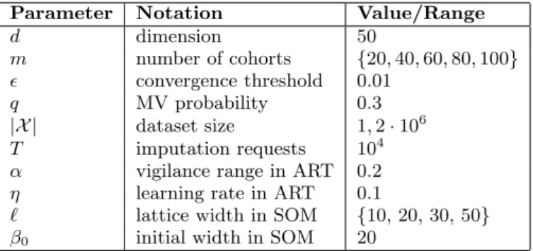
all dimensions in order to construct theP set. We run all experiments 10,000 times and took their average values for all performance metrics. The number of cohortsm ranges in{20, . . . ,100}. Pythia’s cohorts prediction algorithms and the MVAs reported in Section 3.2 were developed in Java. Table 1 summarizes the parameter values used in our exper-iments.
Parameter Notation Value/Range
d dimension 50 m number of cohorts {20,40,60,80,100} convergence threshold 0.01 q MV probability 0.3 |X | dataset size 1,2·106 T imputation requests 104
α vigilance range in ART 0.2
η learning rate in ART 0.1
` lattice width in SOM {10, 20, 30, 50}
β0 initial width in SOM 20
Table 1: Experimental parameters.
5.2
Performance metrics
Our metrics includeefficiency metricsandaccuracy met-rics. A scale-out system consisting ofmcohorts affords two types of parallelism: intra-imputationandinter-imputation
parallelism. The former refers to the capability of process-ing any sprocess-ingle imputation usprocess-ing a number of cohorts in par-allel, each accessing a dataset partition. The latter refers to the systems’ capability of running in parallel a number of imputations, each of which engages a subset of cohorts. It is crucial to note that Godzilla affords neither of these parallelism. This latter scenario is particularly important as typically a system is presented with a (large) batch of (vector-) inputs, each with missing values and the goal is to impute all input vectors in the batch as quickly/scalably as possible. Given this, our efficiency metrics embody various efficiency aspects impacting scalability.
First, we report onimputation latency, defined as the time (in seconds) a system (i.e., Godzilla or Pythia) requires to impute a single input (vector) using a MVA. The rate of latency increase as dataset sizes grow is a strong aspect of scalability. In Pythia, latency refers to the time to predict best cohortS∗, plus the latency to run MVA in parallel at
the engaged cohort.
Imputation speedup is defined as the ratio of Godzilla la-tency over Pythia lala-tency; it indicates how much a system is faster than Godzilla for a single imputation. The linear imputation speedup ratio ism.
We measureimputation accuracyusing the RMSE metric, i.e., the root-mean squared difference between actual vector
xaand estimated vector ˆxafterT imputation requests:
RM SE= 1 T T X t=1 Pd k=1wtk(x(a)tk−xˆtk)2 Pd k=1wtk !1/2 . (6) Finally, we measure thestoragemetricbfor Pythia adopt-ing either ART or SOM signatures. Specifically, this metric refers to the total number of representatives in the ART signature and total number of representatives in the SOM signature. For the latter case, this corresponds tob=`2m
given that all SOM signatures adopt the same lattice width
`. In the ART signature case, each signature has constructed different number of representatives, which depends on the underlying data distribution of each cohort’s dataset. Ifξi
is the number of representatives of an ART signaturePithen
the storage metric corresponds tob=Pm i=1ξi.
5.3
Imputation efficiency
Figures 2 and 3 show the imputation speedup against number of cohortsmusing the EM and KNN imputation al-gorithms, respectively, utilizing Pythia with ART and SOM signatures. In KNN at Figure 3, a slightly super linear speedup is observed for all number of cohorts, e.g., speedup ratio is a slightly greater than m when m cohorts are en-gaged in the imputation process. Super linear speedup is also noticed for EM at Figure 2 when the number of cohorts increases. This is due to the fact that the MVAs algorithms (KNN and EM) highly depend on the size of datasetX, i.e., their computational complexity is proportional to O(|X |). Hence, a portion of dataset|Xi|=m1|X |which is processed
by an imputation algorithm over a cohort Si yields a
de-crease in the corresponding latency of imputation by at least a factor of m. More interestingly, the more demanding (in terms of computational effort) an imputation algorithm is, the more benefit we get if we run it over a portion of the entire dataset; see also Remarks 1 and 2 in Section 3.2 for the computational complexity of the imputation algorithms. Overall, Pythia has achieved substantial speedup using ART and SOM signatures in both MVAs.
Number of cohortsm 20 40 60 80 100 S p ee d u p 0 20 40 60 80 100 120 Pythia (ART) Pythia (SOM) Linear speedup
Figure 2: Speedup vs. number of cohortsmfor ART and SOM signatures using EM.
Number of cohortsm 20 40 60 80 100 S p ee d u p 20 40 60 80 100 120 140 Pythia (ART) Pythia (SOM) Linear speedup
Figure 3: Speedup vs. number of cohortsmfor ART and SOM signatures using KNN,K= 10.
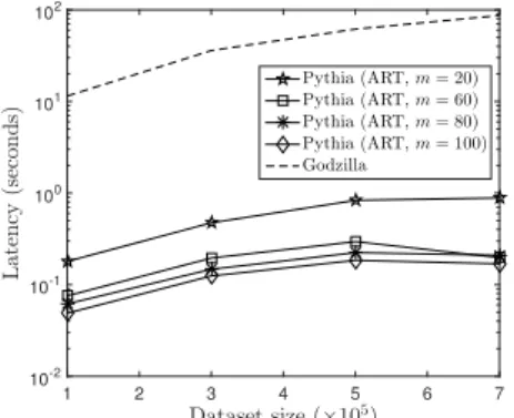
Figures 4 and 5 show the latency in seconds of Godzilla and Pythia for ART and SOM signatures, respectively, in logarithmic scale for different number of cohortsmagainst different number of dataset size|X |. The dataset size varies from 105to 7·105of 50-dimensional vectors. Godzilla
strug-gles with increasing dataset size. Specifically, for Godzilla, by an increasing dataset size, a supper linear increase in latency is observed in both Figures 4 and 5. Pythia scales nicely with its latency increasing linearly utilizing both ART and SOM signatures. Indicatively, given a dataset size|X |= 5·105, Godzilla requires 60 seconds and Pythia (withm=
100 and SOM signature) requires 0.2 seconds to impute an input, respectively. Moreover, when the number of cohorts increases, a sub-linear increase in latency is obtained for Pythia. Pythia can easily handle large datasets if more co-horts are available to scale to big data missing values. Our results up to now clearly make a strong case for the scale-out advantages of the Pythia framework.
Dataset size (×105) 1 2 3 4 5 6 7 L at en cy (s ec on d s) 10-2 10-1 100 101 102 Pythia (ART,m= 20) Pythia (ART,m= 60) Pythia (ART,m= 80) Pythia (ART,m= 100) Godzilla
Figure 4: Latency in seconds vs. dataset size ×105
for Pythia ART and Godzilla with different number of cohortsm={20,60,80,100}.
5.4
Imputation accuracy
We now experiment with the expected achieved imputa-tion accuracy utilizing the most relevant cohorts in parallel. We focus on the best cohort prediction scheme where Pythia based on ART and SOM signatures engages only the best co-hort out of themcohorts. Figures 6 and 7 show the RMSE against the number of cohorts m using KNN and EM, re-spectively. Pythia (in both ART and SOM signatures) using KNN, obtains a relatively low RMSE (on average for allm)
Dataset size (×105) 1 2 3 4 5 6 7 L at en cy (s ec on d s) 10-2 10-1 100 101 102 Pythia (SOM,m= 20) Pythia (SOM,m= 60) Pythia (SOM,m= 80) Pythia (SOM,m= 100) Godzilla
Figure 5: Latency in seconds vs. dataset size ×105
for Pythia SOM and Godzilla with different number of cohortsm={20,60,80,100}.
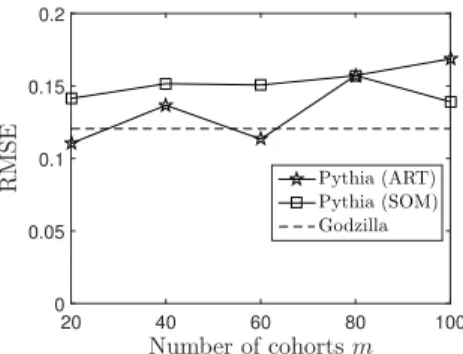
as observed in Figure 6. The same RMSE was also achieved by Godzilla. Accordingly, there was no significant statisti-cal difference observed between the accuracy of Pythia and Godzilla. Please note that Pythia adopting the best cohort prediction scheme and using KNN yields a higher RMSE compared to Godzilla. This is due to the fact that, using KNN, Godzilla would provide the global nearest K points, whereas in Pythia, the best cohort, even when storing irrel-evant data, will be contributing its local nearest K points. The latter necessarily implies that a single-cohort tion might involve points, which adversely affect imputa-tion accuracy. Using EM, however, the lowest and highest RMSE were achieved by Pythia (base on ART signature), 0.11 and 0.16, respectively; see Figure 7. Comparing against the RMSE of Godzilla, 0.12, still there is no significant dif-ference. This indicates that Pythia has comparable RMSE with Godzilla regardless of the imputation algorithms and the signature creation algorithms.
Number of cohortsm 20 40 60 80 100 R M S E 0 0.02 0.04 0.06 0.08 0.1 Pythia (ART) Pythia (SOM) Godzilla
Figure 6: RMSE vs. number of cohortsmfor Pythia ART, Pythia SOM and Godzilla using KNN.
Finally, Table 2 shows the total number of representatives
b=Pm
i=1ξi and representativesb=` 2
min ART and SOM
signatures that are stored in Pythia for making predictions against the number of cohorts m forα = 0.2 and `= 20, respectively; we also show the percentage storage b
|X | with
respect to the entire dataset size. One can observe that, in the case of the ART signature, the average number of representatives per cohort decreases with the number of co-horts. This indicates the robust behavior of Pythia in terms
Number of cohortsm 20 40 60 80 100 R M S E 0 0.05 0.1 0.15 0.2 Pythia (ART) Pythia (SOM) Godzilla
Figure 7: RMSE vs. number of cohortsmfor Pythia ART, Pythia SOM and Godzilla using EM.
of storage requirements. Specifically, the total number of representatives remains the same for all values ofm. In the case of the SOM signature, the number of representatives is explicitly controlled by the`parameter and is not deter-mined by the underlying data distribution. Given a number of cohortsm≤50, by comparing the imputation accuracy of both signature methods, ART and SOM (see also Figures 6 and 7), we observe that a Pythia variant with SOM sig-nature requires 50% less storage than a Pythia variant with ART signature for achieving quite similar accuracy levels for both KNN and EM imputation algorithms. In this case, we can conclude that, when deploying a relatively low num-ber of cohorts for missing values imputation, the adoption of SOM signature is preferable than an ART signature scheme. On the other hand, for a relatively high number of deployed cohorts, both variants (ART and SOM) can be applied with ART signature resulting into slightly better accuracy per-formance and SOM signature requiring 2% less storage.
ART ART pct. SOM SOM pct.
m b=Pm i=1ξi (%)|X |b b=` 2 m (%) b |X | 20 40,047 3.09 8,000 0.61 40 40,630 3.13 16,000 1.23 60 40,813 3.15 24,000 1.85 80 41,153 3.17 32,000 2.47 100 41,190 3.18 40,000 3.08
Table 2: Storage requirement in Pythia.
6.
CONCLUSIONS & FUTURE RESEARCH
We have tackled the problem of scaling out MV impu-tations, a common problem in many big data applications. We studied and developed some of the fundamentals of the problem, based on which we developed Pythia, a framework and algorithms designed for this aim. The Pythia frame-work is drastically different, as it on the one hand avoids the need to access all cohorts (and all associated costs for com-munication and for running MVAs at all cohorts), while on the other can achieve better or comparable MV imputation accuracy, compared to centralized solutions. The major pur-pose of this paper is to examine whether the Pythia frame-work introduced in [1] is robust and independent of any MVA and signature creation algorithm. Specifically, through our comprehensive experiments in this paper we showed that
Pythia can provide drastically better efficiency/scalability and competitive accuracy compared to a centralized ap-proach (Godzilla). This is achieved by introducing the idea of the signature, a statistical learning structure over the dis-tributed datasets. The signatures are exploited by Pythia to decide on the most appropriate subset of data nodes to be access upon a stream of imputation requests. We proposed two methods for constructing a signature structure based on adaptive vector quantization and competitive learning. The central conclusions of our study are as follows. Godzilla suffers from obvious severe scalability and efficiency limita-tions. Hence, Pythia is deemed as an appropriate solution since it not only significantly outperforms Godzilla in terms of efficiency (storage, latency) but, also, performs as good as Godzilla with respect to imputation accuracy. Moreover, the Pythia is independent of any particular imputation al-gorithm and signature construction alal-gorithm. This renders the Pythia framework capable of coping with MV imputa-tion requests, which are directed to subsets of cohorts for local MVA invocations.
6.1
Discussion on Limitations
A primary functionality of the Pythia is the swiftly de-termination of the most relevant subset of cohorts to direct the incoming MV imputation request (input vectori) based on the signatures. In this context, the Pythia node decides on the closest representative c of each cohort’s signature by calculating the Euclidean distance over the dimensions of the input that contain non-missing values. In the case of high-dimensional data (dis relatively high) and when the probability of a missing value is low (pis relatively low) then the Pythia node has to calculate the Euclidean distance over (1−p)d dimensions. In that case, the Euclidean distance metric might change in some non-obvious ways [31]. Specif-ically, as it has been argued in [32], under certain reasonable assumptions on the underlying data distribution, the ratio of the distances of the nearest and farthest neighbors to a given target in a high dimensional space is almost unity for a wide variety of data distributions and distance functions. In such a case, the nearest neighbor identification (which refers to the closest representative in our context) becomes ill defined, since the contrast between the distances to dif-ferent data points does not exist. In such cases, even the concept of proximity may not be meaningful from a qualita-tive perspecqualita-tive: a problem which is even more fundamental than the performance degradation of high dimensional al-gorithms. In our case, theLk= (Pdj=1(ij−cj)k)1/knorm
with k = 2, i.e., L2 = (Pdj=1(ij−cj)2)1/2 is susceptible
to the dimensionality curse for many classes of data distri-butions [32]. Specifically, based on the analysis in [32], the relative contrast of the distance of an input vectoriwith a representative vectorc depends heavily on the adoptedLk
distance metric. This provides considerable evidence that the meaningfulness of the Lk norm worsens faster with
in-creasing dimensionality for higher values ofk. Thus, in our problem with a high value of the dimensionalityd, it may be preferable to use lower values ofk. This means that theL1
distance metric (i.e., the Manhattan distance metric) is the most preferable for high dimensional applications, followed by the Euclidean (L2), then theL3 metric, and so on.
En-couraged by the analysis in [32], we are planning, as a future work, to examine the behavior offractionaldistance metrics for the distance between i and c, in whichk is allowed to
be a fraction smaller than unity. Further, the limitations of the adopted algorithms for the signatures construction and the possible directions for dealing with these limitations are discussed in Section 4.4.
6.2
Future Research
Apart from the future work discussed in Sections 4.4 and 6.1 triggered by the limiations of the Pythia framework, we further plan to incorporate to our research agenda the fol-lowing items. This work has shown that the Pythia frame-work improves not only the imputation efficiency but also achieves at least the same imputation accuracy comparing against the performance of the Godzilla variant. The exper-imental evaluation focuses on stationary data. In station-ary data, the underlying probability distribution function does not change over time. Hence, the signatures of the Pythia do not change frequently so that they remain as a reliable representation (through the derived clusters). In a non-stationary data environment, e.g., an environment deal-ing with data streams, such distribution function (estimated through clusters) changes over time swiftly [30]. In this con-text,newclusters can be formated andexistingclusters have to be updated to follow the data streams trend. Therefore, our future research items include the enhancement of the Pythia framework to access only a relevant part of the whole dataset in order to improve scalability, efficiency and predic-tion accuracy in a dynamic environment with ever-changing data patterns. As the probability distribution function of the data streams changes frequently, we plan to investigate methods for updating the Pythia signatures to efficiently support MV imputation requests.
7.
REFERENCES
[1] C. Anagnostopoulos,et al, Scaling out big data missing value imputations: pythia vs. godzilla.Proc. 20th ACM SIGKDD (KDD’ 14) International Conference on Knowledge discovery and data mining. ACM, New York, NY, USA, pp.651–660.
[2] X. Su,et al, ‘Using Classifier-Based Nominal
Imputation to Improve Machine Learning’,Proc. 15th PAKDD, Part I, LNAI 6634, pp. 124–135, 2011. [3] A. Farhangfar,et al, ‘Impact of imputation of missing
values on classification error for discrete data’,Pattern Recognition, 41(12): 3692–3705, Dec 2008.
[4] M.T. Asif,et al, ‘Low–Dimensional Models for Missing Data Imputation in Road Networks’,Proc. 38th IEEE ICASSP, pp.3527–3531, 2013.
[5] T. Kohonen. 2001. ‘Self-Organizing Maps’ (3rd ed.). Springer-Verlag New York, Inc., Secaucus, NJ, USA. [6] E.C. Chi,et al, ‘Genotype imputation via matrix
completion’,Genome Research, 23(3):509–18, Mar 2013.
[7] I.B. Aydilek,et al, ‘A novel hybrid appoach to estimating missing values in databases usingk–nearest neighbors and neural networks’,Innovative
Computing, Information and Control, 8(7A): 1349–4198, Jul 2012.
[8] A. Farhangfar,et al, ‘A Novel Framework for Imputation of Missing Values in Databases’,IEEE Trans. Sys. Man Cyber. (A), 37(5): 692–709, Sep 2007. [9] K. Lakshminarayan,et al, ‘Imputation of missing data in industrial databases’,Appl. Intell., 11(3): 259–275,
Nov / Dec 1999.
[10] L. A. Kurgan,et al, ‘Mining the cystic fibrosis data’, J. Zurada & M. Kantardzic (Eds.),Next Generation of Data–Mining Applications, IEEE Press, 415–444, 2005. [11] A.W. Liew,et al, ‘Missing value imputation for gene
expression data: computational techniques to recover missing data from available information’,Brief. Bioinform., 12(5): 498–513, Sep 2011.
[12] J. Dean,et al, ’MapReduce: Simplified Data Processing on Large Clusters’,Proc. USENIX OSDI, 2004.
[13] S. Ghemawat,et al, ‘The Google File System’,Proc. ACM SOSP, 2003.
[14] C-T. Chu,et al, ‘Map-Reduce for Machine Learning on Multicore’,NIPS 19, MIT press, 281–288, 2006. [15] C. K. Enders, ‘Applied Missing Data Analysis’,
Guilford Press, NY, 2010.
[16] D. W. Joenssen,et al, ‘Hot Deck Methods for Imputing Missing Data’,Proc. 8th MLDM, LNCS 7376, pp.63–75, 2012.
[17] O. Troyanskaya,et al, ‘Missing value estimation methods for DNA microarrays’,Bioinformatics, 17(6):520–525, 2001.
[18] R.J. Little,et al, ‘Statistical Analysis with Missing Data’,Wiley, NY, 1987.
[19] T.E. Raghunathan,et al, ‘A multivariate technique for multiply imputing missing values using a sequence of regression models’,Survey Methodology, 27(1):85–95, 2001.
[20] D.B. Rubin, ‘Multiple Imputation After 18+ Years’,J. of the American Statistical Association,
91(434):473–489, 1996.
[21] L. Li,et al, ‘DynaMMo: mining and summarization of coevolving sequences with missing values’,Proc. 15th KDD, 527–534, 2009.
[22] S. Yang,et al, ‘Online recovery of missing values in vital signs data streams using low–rank matrix completion’,Proc. 11th IEEE ICMLA, 281–287, 2012. [23] M. Ouyang,et al, ‘Gaussian mixture clustering and
imputation of microarray data’,Bioinformatics, 20(6): 917–923, Apr 2004.
[24] T. Aittokallio,et al, ‘Dealing with missing values in large-scale studies: microarray data imputation and beyond’Brief. Bioinform.11(2):253–264, 2010. [25] D-W. Kim,et al, ‘Iterative Clustering Analysis for
Grouping Missing Data in Gene Expression Profiles’,
Proc. PAKDD 2006, LNAI 3918, pp.129–138, 2006. [26] G. A. Carpenter,et al, ‘The ART of adaptive pattern
recognition by a self–organizing neural network’,IEEE Computer, 21(3): 77–88, Mar 1988.
[27] L. Meng,et al, ‘Vigilance adaptation in adaptive resonance theory’Neural Networks (IJCNN), IEEE International Joint Conference on, pp.1–7, 2013. [28] Y. Prudent,et al‘An incremental growing neural gas
learns topologies’Neural Networks (IJCNN), IEEE International Joint Conference on, vol.2, no., pp.1211–1216, 2005.
[29] A. Ahmad,et al, ‘Ak–mean clustering algorithm for mixed numeric and categorical data’Data & Knowledge Engineering, 63(2):503–527, 2007. [30] Y. Chen and L. Tu. Density-based clustering for
real-time stream data. InProceedings of the 13th ACM SIGKDD International Conference on Knowledge Discovery and Data Mining, 133–142, ACM, 2007. [31] C. Aggarwal,et al, On the surprising behavior of
distance metrics in high dimensional space.Springer. 2001.
[32] K. Beyer,et al.‘When is Nearest Neighbors Meaningful?’ ICDT Conference Proceedings, 1999. [33] K. Bache,et al, UCI Machine Learning Repository
[http://archive.ics.uci.edu/ml] Irvine, Uni. of California, School of Inform. and Comp. Sci., 2013.