Frequency dependence of hysteresis curves in conducting magnetic materials

Ames Laboratory Publications

Ames Laboratory

11-15-1994

Frequency dependence of hysteresis curves in

conducting magnetic materials

David C. Jiles

Iowa State University, [email protected]

Follow this and additional works at:

http://lib.dr.iastate.edu/ameslab_pubs

Part of the

Electromagnetics and Photonics Commons

, and the

Engineering Physics Commons

The complete bibliographic information for this item can be found at

http://lib.dr.iastate.edu/

ameslab_pubs/159

. For information on how to cite this item, please visit

http://lib.dr.iastate.edu/

howtocite.html

.

Frequency dependence of hysteresis curves in conducting magnetic

materials

Abstract

An extension of the hysteresis model has been developed that takes into account the effects on the hysteresis

curves of eddycurrents in electrically conducting media. In the derivation presented it is assumed that the

frequency of the applied field is low enough (or the thickness of the material medium small enough) that the

skin effect can be ignored so that the magnetic field penetrates uniformly throughout the material. In this case,

the dc hysteresis equation is extended by the addition of a classical eddy‐current‐loss term depending on (i)

the rate of change of magnetization with time, (ii) the resistivity of the material, and (iii) the shape of the

specimen; and on an anomalous (or excess) eddy‐current‐loss term which depends on (

dB

/

dt

)

3/2

. In the

limit, as the frequency of the magnetic field tends to zero, the frequency‐dependent hysteresis curve

approaches the dc curve.

Keywords

Magnetic hysteresis, Magnetic materials, Electrical hysteresis, Magnetic fields, Alternating current power

transmission

Disciplines

Electromagnetics and Photonics | Engineering Physics

Comments

The following article appeared in

Journal of Applied Physics

76 (1994): 5849 and may be found at

http://dx.doi.org/10.1063/1.358399

.

Rights

Copyright 1994 American Institute of Physics. This article may be downloaded for personal use only. Any

other use requires prior permission of the author and the American Institute of Physics.

Frequency dependence of hysteresis curves in conducting magnetic materials

D. C. Jiles

Citation: Journal of Applied Physics 76, 5849 (1994); doi: 10.1063/1.358399

View online: http://dx.doi.org/10.1063/1.358399

View Table of Contents: http://scitation.aip.org/content/aip/journal/jap/76/10?ver=pdfcov

Published by the AIP Publishing

Articles you may be interested in

A modified Preisach hysteresis operator for the modeling of temperature dependent magnetic material behavior

J. Appl. Phys. 109, 07D338 (2011); 10.1063/1.3562520

Amplitude and frequency dependence of hysteresis loss in a magnetsuperconductor levitation system J. Appl. Phys. 78, 2097 (1995); 10.1063/1.360187

Erratum: ‘‘Frequency dependence of hysteresis curves in conducting magnetic materials’’ [J. Appl. Phys. 76, 5849 (1994)]

J. Appl. Phys. 77, 4834 (1995); 10.1063/1.359615

Frequency dependence of hysteresis curves in conducting magnetic materials (abstract) J. Appl. Phys. 75, 5511 (1994); 10.1063/1.355672

On the Relation Between Magnetization Curves and Hysteresis Loops Am. J. Phys. 1, 121 (1933); 10.1119/1.1992846

Frequency

dependence

of hysteresis

curves in conducting

magnetic materials

D. C. Jiles

Ames Laboratory, Iowa State Universiq, Ames, Iowa 50011

(Received 12 January 1994; accepted for publication 4 August 1994)

An extension of the hysteresis model has been developed that takes into account the effects on the hysteresis curves of eddy currents in electrically conducting media. In the derivation presented it is assumed that the frequency of the applied field is low enough (or the thickness of the material medium small enough) that the skin effect can be ignored so that the magnetic field penetrates uniformly throughout the material. In this case, the dc hysteresis equation is extended by the addition of a classical eddy-current-loss term depending on (i) the rate of change of magnetization with time, (ii) the resistivity of the material, and (iii) the shape of the specimen; and on an anomalous (or excess) eddy-current-loss term which depends on (~@ldf)~‘~. In the limit, as the frequency of the magnetic field tends to zero, the frequency-dependent hysteresis curve approaches the dc curve.

I. INTRODUCTION

The hysteresis model equation used in this work has been described previous1y.r” The hysteresis equation can be used to describe both major (symmetric) loops and minor (asymmetric) 100~s.~ Previously, the model equation has been extended to take into account the change in shape of hysteresis loops under a constant applied stress.5 The earlier work on the development of the hysteresis model was con- cerned with quasistatic or dc hysteresis loops. The model is based on the concept of the anhysteretic, which provides a global optimum macroscopic state for the magnetization of a material subjected to a magnetic field. The equation for the anhysteretic magnetization was derived, and this resulted in the following expression:

M,,(H) =M,B f

H+ aM,(H) a _i 2

where qx) is the Langevin function,

2&?$) = coth x- l/x. ₍₂₎

In IQ. (l), M,(H) is the anhysteretic magnetization un- der an applied field H, M, is the saturation magnetization, a is a coupling coefficient which arises from the exchange in- teraction, and a = kBT/puo(m), where kB is Boltzmann’s con- stant (1.38X1O-23 J K-r), T is the temperature in K, ,uo is the permeability of free space (4rX 10V7 H ml), and (m) is the effective domain size. This (m) is the size of a typical do-

main in a classical ferromagnetic Ising array with a mean- field interaction which obeys the Langevin equation. The pa- rameter a is therefore proportional to the effective domain density and the absolute temperature.

The equation for hysteresis can be derived from an energy-balance equation in which the magnetic energy sup- plied, for example, to an initially demagnetized material, can appear either as a change in total magnetization M (magne- tostatic energy), or be dissipated due to irreversible changes in magnetization Mi, (hysteresis loss). If there is no dissipa- tion (hysteresis) then, by definition, the magnetization must

follow the anhysteretic {hysteresis-free) curve. In the pres- ence of hysteresis, the energy-balance equation is

PO

_{I Ma,}

dff,=~uo

_I

M dH,

+p,k&l-c) (3)

where the first term of the right-hand side is the contribution to the magnetostatic energy, and the second term on the right-hand side is the dissipation loss due to pinning. In this equation H,= H + CYM, the coefficient k is the pinning pa- rameter which determines the amount of energy dissipated, and 6 is a directional parameter which ensures that energy is always lost through dissipation. S= + 1 when dHldt> 0 and S= - 1 when dHldt<O. The coefficient c is a measure of the amount of reversible change in magnetization, as is dis- cussed shortly. Under quasistatic or equilibrium conditions, energy losses arise only from changes in the irreversible magnetization Mh. The irreversible magnetization is the component of magnetization that would remain if all domain walls were relaxed back to the planar state and all reversible rotations were reset.

The irreversible and reversible components of magneti- zation can be separated by differentiating Eq. (3). Since M=Mh+M,,,,

dMim

M,=Mi~+hf,,+kS(l-~) ~7 e

and simply by considering that if c= 0 and M,,=O, it fol- lows that

dMh Min=Man-ka do,

and

M,,=c(M,-Mh). (6)

J. Appl. Phys. 76 (IO), 15 November 1994 0021-8979/94/76(10)/5849/7/$6.00 0 1994 American Institute of Physics 5849

Equations (5) and (6) are the basic equations of hyster- esis which have been given previously,6 and the energy equa- tion (3) can be derived directly from them.

The rate of change of magnetization with field dMldH is then dependent on the displacement of the magnetization from the anhysteretic. In order that the pinning always gives rise to a loss of energy (i.e., is dissipative), this dependence on the displacement M,(H)-Mi,,(H) applies when the magnetization is below the anhysteretic and the field is in- creasing (Man>Mi= and dH/dt>O) and when the magneti- zation is above the anhysteretic and the field is decreasing (M,<Mi, and dH/dt<O).

The differential susceptibility dMJdH can be expressed as a sum of the irreversible and reversible components,

dM(H) dMirr(H) + dMrev(H)

-=

dH dH dH ’

where M&H) is the irreversible component of magnetiza- tion and M,,(H) is the reversible component of magnetiza- tion. This leads to the differential equation for hysteresis,6

dWH)

M,(H) -Mi&O

-=

dH k& a[M,(H) -M(H)]

Man(H) -MinW)

- kc% a[M,(H) - M(H)] (8)

where the terms on the right-hand side are, respectively, the irreversible and reversible differential susceptibilities. The term c, which determines the amount of reversible magneti- zation, is derived from the amount of domain-wall bending7 and is dependent on the domain-wall surface energy.

II. OBJECTIVE OF THE PRESENT WORK

Recently it has been shown how the frequency depen- dence of hysteresis can be described in “nonconducting” media, such as high-frequency ferrites, through a second- order differential equation.8 In the present work, the hyster- esis equation is extended to describe the frequency depen- dence of hysteresis in electrically conducting materials. In this extension of the model to account for these effects it is assumed, for the sake of simplicity, that the magnetic field penetrates the entire cross-sectional area of the material uni- formly. In most practical cases, the frequency of operation of electrically conducting magnetic media, such as transformer or motor laminations, is much lower than for nonconducting magnetic media, such as high-frequency inductor cores. Therefore, the effects of magnetic relaxation and resonance which have been described in a previous article* can be ig- nored and these phenomena can be entirely separated from the effects of eddy currents. Furthermore, the cross sections of laminations are chosen so that the thickness is compa- rable, or less than, the depth of penetration of the magnetic field, to ensure high penetration of the field throughout the volume of material.

III. DERIVATION OF THE FREQUENCY-DEPENDENT HYSTERESIS EQUATION

Additional energy dissipation resulting from eddy cur- rent losses that arise in electrically conducting media can be added to the right-hand side of Eq. (3) and will thereby lead to a modification of the hysteresis loops with the rate of change of field dHldt.

The approach taken in this work is to determine the in- stantaneous power losses due to eddy currents, and then to include these in the energy-balance equation given above. The power losses are therefore separated into hysteresis loss dW,ldt, classical eddy current loss dW,,ldt, and anoma- lous (or excess) loss d WJdt. The classical eddy current loss is obtained by solving the Maxwell equation VXE = -dBl dt for a given geometry, assuming that the magnetic field penetrates uniformly throughout the material.

The classical eddy current instantaneous power loss per unit volume is proportional to the square of the rate of change of magnetization as discussed by Chikazumi.’ This gives

(9)

Where p is the resistivity in fl m, d is the cross-sectional dimension in meters (thickness for laminations, diameter for cylinders and spheres) and p is a geometrical factor which varies from /?=6 in laminations to p=16 in cylinders and /?=20 in spheres. The approximation B =,q,M, which is valid for soft magnetic materials, has been made in Eq. (9). Under the restricted condition of sinusoidal variation of B with time, at moderate and low frequencies of magnetic-field excitation, such that the flux penetration is complete, the eddy current power loss per unit volume becomes equal to the well-known expression”

d WEc rr2B2 d2 2 max

f

-=

dt _{PP ’} (10)

where B,, is the peak flux density in the cycle and

f

is the frequency in Hz.

The anomalous loss results from domain-wall motion during changes in the domain configuration, and this has been treated in detail by Bertotti11-13 and Fiorillo and Novikov.14 In many cases, this component of the loss can be expressed as

d? -(GyiJo)l’2(

g)3’2,

₍₁₁₎

where G is a dimensionless constant of value 0.1356, w is the width of laminations, d the thickness, p the resistivity, and Ho is a parameter representing the fluctuating internal poten- tial experienced by domain walls. Ho has dimensions of A m-l and so is equivalent to a magnetic field.

Incorporating the eddy-current-loss mechanisms into the theory of hysteresis allows perturbations to the hysteresis curve arising from eddy current losses to be modeled. The energy Eq. (3) which forms the starting point of the deriva- tion of the hysteresis equations can be extended to

5850 J. Appl. Phys., Vol. 76, No. 10, 15 November 1994 D. C. Jiles

+g;iF,.

dMau

M,“(H)=M(H)+ka

z--k& dH,

_{( i}

e’

PO M,W)dH,

_I

W)

where the final two terms on the right-hand side are the clas- sical eddy current loss and the anomalous loss.

This equation needs to be modified slightly before pro- ceeding further,

Mi,=& (M-GM,), 03)

and therefore Eq. (12) becomes

PO ManW)dHe

_I

(14)

A. Case 1: Classical loss only

In the case of a material in which the classical loss is the dominant frequency-dependent term, the quasistatic hyster- esis model can be extended using a perturbation of the hys- teresis equation. In other words, we set Ho equal to 0 in Eq. (14). The differential equation now needs to be converted into a manageable form.

Therefore, replacing (dM/dt)2dt by (dMldt)(dMl dH,)dH,, gives

Substituting this back into the hysteresis equation, and divid- bis by PI-,>

+$ j- (f)(~)dK

Differentiating with respect to H, ,

J. Appl. Phys., Vol. 76, No. 10, 15 November 1994

W-5)

(17)

Equation (17) is equivalent to the quasistatic hysteresis equation with the addition of the final term on the right-hand side. The equation can now be rearranged. Let

(18)

so that under dc conditions k’ = k8, and the difference be- tween k and k’ depends on dMldt.

dM _dM,n

M,,(H)=M(H)+k’ =-kSC =.

₍₁₉₎

It can then be seen that the effects of the classical eddy currents can be incorporated into a modified energy-loss pa- rameter k’ while maintaining the same form of hysteresis equation

dM M,,(H)-M(H)+k& 2

e (20)

and substituting H, = H + aM gives

dM M,(H) - M(H) + k&(dM,ldH,) dH= k’-a[M,(H)-M(H)+kSc(dM,,/dH,)]’

w which gives an equation for the differential susceptibility as a result of both hysteresis and classical eddy currents that is analogous to the equation obtained under quasistatic hyster- esis conditions. The equivalent expressions to Eqs. (5) and (6) for the irreversible and reversible components of magne- tization are

Mrdff) =~[Man(H)-MdfOl*

(23) In order to determine dM/dH, Eq. (21) can be reduced to a quadratic,

($~)(~i”+[k&aiM,.--M+k& $$)I g

dM,,

- Ma,--M+kScz ₍₂₄₎

which can then be solved directly.

In most cases, the external excitation on a material, that is the magnetic field H generated by an electrical current in a solenoid, can be controlled and known, and is often sinu- soidal. Therefore, this form of Eq. (24) can be used to cal- culate the effects on the hysteresis curve of various different, but known, dependencies of magnetic field on time dHldt, such as sinusoidal or triangular field wave forms. On the other hand the response of the material dBldt is dependent on the magnetic properties of the material and is rarely sinu- soidal, as mentioned by Fiorillo and N0vik0v.l~ Equation

D. C. Jiles 5851

(24) therefore provides a means of calculating the time de- pendence of M(t) [and hence B(t)] under a given form of external excitation H(t) for situations in which the dominant eddy current power loss term is the classical loss.

B. Case 2: Classkl and anomalous losses

In those cases where both types of losses are involved, the presence of the excess loss term depending on (dMldt)3’2 in Eq. (12) makes it impossible to get an expres- sion for dM/dH in the same form as Fq. (24). Therefore, the solution is a little more difficult but can be achieved by nu- merical methods.

-I

Beginning again from Eq. (12) and making the same substitution for (dM/dt)2 dt, leads to

I

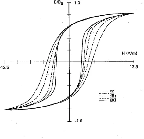
MaaWWe l-I.0

M(H)dH,+kS(l-c) FIG. 1. Measured hysteresis curves of Pennalloy 80 at dc, 400, 1000, 3000,

and 6000 Hz (see Ref. 15).

Differentiating this equation gives the following:

(w) (~~,~~~~~~~)~~~~~~~~~~~~3’2

- -dH

(oqy)+,;$ (ci~)(ci~) -(M,(H)-M(H)+k~c %)=O-= (30)

+~lj$$$f-)d&

+( Gdw;oHo)1’2j- (,)I” gdH,.

M,(H)=M(H)+kS(l-c) - -

+(

GdwyHojliz(

q”( g), (26)

This equation can then be solved for dMfdH using nu- merical methods, and from the- solution the frequency- dependent hysteresis curve can be calculated.

and using the expression for Mi, in Eq. (13), Ill. RESULTS

dM M,(H)=M(H)+kag-k& e

e e

+5$$z)(~)

+( G~yy1’2pLf)1’2(

!K),

₍₂₇₎

which is equivalent in form to the standard quasistatic hys- teresis equation

M,,(H)=‘M(H)+k’? (28)

where the energy-loss parameter k” is now

k”=k+

Equation (27) can then be rearranged in terms of the differential susceptibility dMfdH to give

Permalloy 80 was chosen as a widely used material for testing the agreement between the model predictions and measured properties. The hysteresis curves of Permalloy 80 measured at various frequencies are given in Fig. 1. From the dc hysteresis curve, the magnetic properties were determined and these are shown in Table I. The hysteresis parameters for the model equation were determined from these measured

TABLE I. Comparison of measured and modeled magnetic properties of square Pennalloy 80.

Measured Saturation magnetic induction

Anhysteretic permeability Initial permeability Field at loop tip

Magnetic induction at loop tip Differential permeability at loop tip Magnetic induction at remanence Differential permeability at remanence Coercivity

Differential permeability at coercive point

1.05 T . . . 26X103 12.8 A/m

0.8 T 1.9x103

0.62 T 23xIo3 2.4 A/m 0.73 x lo6

Modeled 1.0 T -0.56X lo6

24x103 12.5 A/m

0.8 T 8.1X103

0.61 T 43x103 2.7 A/m 1.2x106

5852 J. Appl. Phys., Vol. 76, No. 10, 15 November 1994 D. C: Jiles

[image:7.579.30.547.24.732.2]

I iI : i :I ’ / H (A/m)

FIG. 2. Modeled hysteresis curves of Pennalloy 80 at dc, 400, 1000, 3000, and 6000 Hz calculated by incorporating effects of classical eddy current power losses into the hysteresis equation.

properties using the methods described previously.6 The model hysteresis loop was then calculated under quasistatic conditions and the values of the modelled magnetic proper- ties of Permalloy 80 obtained from the solution of the equa- tion are also shown in Table I.

The modeled hysteresis curves were calculated first us- ing only the classical eddy current contribution and then us- ing both classical and anomalous (or excess) eddy current contributions. The hysteresis curves obtained by considering only the classical eddy currents are shown for various differ- ent frequencies in Fig. 2. These show a progressive widening of the hysteresis loops as the frequency was increased, lead- ing ‘to higher coercivity. The dependence of coercivity on frequency, according to the model calculations, is shown in Table II together with the measured values at the same fre- quency.

The measured hysteresis curves show two other features of interest. The remanence remains independent of the fre- quency of excitation, and the loop tips show no evidence of “rounding” as the field is reduced from its maximum excur- sion. Both of these features also result naturally from the model calculations.

However, one feature of the calculations based solely on the effects of classical eddy currents did not give such good agreement with observation; this was the numerical values of the coercivity at higher frequencies. At 6 kHz the discrep- ancy was 1.5 A m-r in a coercivity of 5.9 A m-t. Therefore the effects of anomalous (or excess) eddy currents were in- corporated into the calculation. The results are shown in Fig. 3. In this case the increase in coercivity with frequency is more accurately modeled, as shown in Table II, while the invariance of remanence with frequency and the sharpness of the recoils at the loop tips are maintained.

TABLE II. Comparison of measured and modeled values of coercivity of square Permalloy 80 at different frequencies. These values were obtained using the following model parameters: B,=l T, a=3.75 Am-‘; k=2.4 Am-‘; c~=1.5XlO-~; c = 0.35. For classical losses the following additional parameters were used: p=0.57X10-6 am; d=15X10W6 m; B=6. For anomalous (or excess) losses the following additional parameters were used: w=O.O05 m; Ha=0.0.075 Am-‘.

H, (A m-l) Modeled Frequency (Hz) Measured

Classical loss only

Classical + excess losses dc 2.4 2.4 2.5

400 2.9 2.8 3.5 1000 3.6 3.1 4.0

3000 4.6 3.7 4.9 6000 5.9 4.4 5.6

IV. CONCLUSlONS

The work presented here shows how the hysteresis equa- tion can be extended to account for energy losses resulting from the generation of eddy currents in electrically conduct- ing media. The model represents a first approximation in which the skin effect is ignored, or equivalently the field penetration is assumed to be uniform throughout the mate- rial. This means that the calculations are really only appli- cable to thin laminations.

Both classical and excess eddy current losses have been included in the model, and these appear as different terms in the energy-balance equation (25). The results show some in- teresting features, including the increase in coercivity with frequency, the increase in energy loss per cycle, the invari-

FIG. 3. Modeled hysteresis curves of Permalloy 80 at dc, 400, 1000, 3000, and 6000 Hz calculated by incorporating effects of both classical and anomalous (or excess) eddy current power losses into the hysteresis equa- tion.

J. Appl. Phys., Vol. 76, No. IO, 15 November 1994 D. C. Jiles 5853

[image:8.578.40.276.29.256.2] [image:8.578.297.546.92.263.2] [image:8.578.306.537.438.666.2]

ante of remanence with frequency, and the persistence of total magnetization M, whereas the hysteresis loss depends sharp reversal points at the loop tips, as distinct from the on Mi, . As we shall see, compared with earlier derivations, rounding of the hysteresis curves observed in high-frequency this merely results in a scaling correction to k, which ferrites where were modeled via a relaxation mechanism. amounts to multiplying k by a constant.

Differentiating the above equation, The model provides a relatively simple way of predict-

ing the changes in hysteresis curves as a result of eddy cur- rents at different frequencies. The information needed to cal- culate the hysteresis curves where only classical eddy current losses occur is limited to the dc hysteresis curve of the ma- terial, the resistivity, and the shape of the component (e.g., lamination, cylinder), including its cross-sectional width (e.g., lamination thickness or cylinder diameter). In order to calculate hysteresis curves in the presence of excess eddy current losses, additional information is needed, including the width of the laminations and the field parameter repre- senting the Auctuating internal potential experienced by the domain walls.

dMi#) M,iH)=MiH)+k~ dH ,

E (A4)

and from previous result8

M(H) = (1 - c)M&H) + CM,(H), WI

and therefore, rearranging Eq. (A4) with this substitution leads to

k8 dMi,(H)

Man(H) =MirriH) + (I_ c) dH, 7

iA6)

Future work should include a means of correcting these

curves for the effects of the depth of penetration of the mag- netic field, or skin depth, in conducting media. This would enable the model to be extended to “thick” components in which the energy dissipation at a given frequency was not uniform over the entire cross section.

which is identical to previous equations except for the l/(1 -c) factor, which effectively leads only to a scaling of k. Equation (A6) is an exact derivative of the energy-balance equation (A3). It can be manipulated into an expression for the differential susceptibility dM,(H)/dH which is particu- larly useful for calculating hysteresis curves. Equation (A6) can be shown to be exactly equivalent to

ACKNOWLEDGMENTS

This work was supported by the U.S. Department of En- ergy, Office of Basic Energy Sciences, Division of Materials Sciences, under Contract No. W-7405ENG-82. The author wishes to thank Dr. G. Bertotti for useful discussions which have led to a more general exposition of the eddy current losses within the hysteresis model presented here, and Mag- netics Technology, Inc. for use of proprietary hysteresis mod- eling software.

APPENDIX: ENERGY-BALANCE EQUATION FOR QUASISTATIC HYSTERESIS

In the absence of time-dependent effects, the energy bal- ance equation is given by

energy supplied=change in magnetostatic energy

fenergy dissipated. _iAl)

If there is no hysteresis, then the energy dissipated is zero and consequently the magnetization follows the anhys- teretic. Therefore,

I PoM,W)dH,= I POWWH,; WY

where H, = H + CH is used instead of H because of the need to include internal coupling energy. If there is hysteresis, then this hysteresis arises from irreversible changes in mag-

netization M,, and therefore the most precise form of the energy equation for hysteresis is

I ~oMan(H)dHe= I /~oMifWH,+k&~o I dMim(W iA% using the notation described in the text. The important dif- ference here is that the magnetostatic energy depends on the

dMir#O

M,(H) -MirrW)

dH = k6

(1-c)- dM,W) -MiAff>l g

in

(A7) Now it has also been shown elsewhere2 that

M=Min+M,,, _w>

=(l-c)M,+cM,, _(A9)

and therefore for small values of c it follows that dMldM,*l, and therefore Eq. (A7) becomes equal to the equation for the irreversible differential susceptibility that has been quoted beforeP namely

dMirr(W

M&O -MirriW

dH = [kLV(l -c)] - a[M,(H) -Mb(H)]

iAl01

and when summed with the reversible differential suscepti- bility,

dMrw dManV-0 dMiAf8

dH=c dH - dH ’ (All)

so that the total differential susceptibility becomes

d:f’ -(1-c> ks M.&O-MirrW

~-

4ManW) - Mirr(H)

1

(1-c)

+c dM,iH)

dH ’ 6412)

Another possibility that has not been fully explored is what happens when c is not small, so that dMldMh#l, and the approximations leading to Eq. (A12) cannot be made. The only known case in this situation is c= 1, when the solution is simply M(H)=M,(H).

5854 J. Appl. Phys., Vol. 76, No. 10, 15 November 1994 D. C. Jiles

‘D. C. Jiles and D. L. Atherton, J. Appl. Phys. 552115 (1984). ‘D. C. JiIes and D. L. Atherton, J. Magn. Magn. Mater. 61, 48 (1986). 3D. C. JiIes and J. B. Thoelke, IEEE Trans. Magn. MAG-253928 (1989). 4D. C JiIes, IEEE ‘Darts. Magn. MAG28, 2603 (1992).

5D. A. Kaminski, D. C. Jiles, and M. J. Sablik, J. Magn. Magn. Mater. 104, 382 (1992).

“D. C. JiIes, J. B. Thoelke, and M. K. Devine, IEEE Trans. Magn. MAG- 28, 27 (1992).

7D. C. Jiles, in 37th Annual Conference on Magnetism and Magnetic Ma- terials, Houston, 1992; J. Appl. Phys. 73, 5854 (1993).

J. Appl. Phys., Vol. 76, No. 10, 15 November 1994

8D. C. Jibes, IEEE Trans. Magn. MAG-29, 3490 (1993).

9S. Cbikazumi, Physics of Magnetism (Wiley, New York, 1964), p. 321. “D. C. JiIes, Introduction to Magnetism and Magnetic Materials (Chapman

and HalI, London, 1991), p. 271. “G. Bertotti, J. Appl. Phys. 55, 4339 (1984). “G. Bertotti, J. Appl. Phys. 57, 2210 (1985).

t3G. Bertotti, IEEE Trans. Magn. MAG-24, 621 (1988).

14F. Fiorillo and A. Novikov, IEEE Trans. Magn. MAG-26, 2904 (1990). “Design Manual for Tape Wound Cores (Magnet& Inc., 1987), p. 37.

D. C. Jiles 5855