Pseudorandom Generators from
One-Way Functions:
A Simple Construction for Any Hardness
Thomas Holenstein
ETH Zurich, Department of Computer Science, CH-8092 Zurich [email protected]
Abstract. In a seminal paper, H˚astad, Impagliazzo, Levin, and Luby showed that pseudorandom generators exist if and only if one-way func-tions exist. The construction they propose to obtain a pseudorandom generator from an n-bit one-way function uses O(n8) random bits in
the input (which is the most important complexity measure of such a construction). In this work we study how much this can be reduced if the one-way function satisfies a stronger security requirement. For exam-ple, we show how to obtain a pseudorandom generator which satisfies a standard notion of security using onlyO(n4
log2(n)) bits of randomness if a one-way function with exponential security is given, i.e., a one-way function for which no polynomial time algorithm has probability higher than 2−cn in inverting for some constantc.
Using the uniform variant of Impagliazzo’s hard-core lemma given in [7] our constructions and proofs are self-contained within this paper, and as a special case of our main theorem, we give the first explicit description of the most efficient construction from [6].
1
Introduction
A pseudorandom generator is a deterministic function which takes a uniform random bit string as input and outputs a longer bit string which cannot be distinguished from a uniform random string by any polynomial time algorithm. This concept, introduced in the fundamental papers of Yao [16] and Blum and Micali [1] has many uses. For example, it immediately gives a semantically se-cure cryptosystem: the input of the pseudorandom generator is the key of the cryptosystem, and the output is used as a one-time pad. Other uses of pseu-dorandom generators include the construction of pseupseu-dorandom functions [2], pseudorandom permutations [11], statistically binding bit commitment [13], and many more.
Such a pseudorandom generator can be obtained from an arbitrary one-way function, as shown in [6]. The given construction is not efficient enough to be used in practice, as it requiresO(n8) bits of input randomness (for example, if one would like to have approximately the security of a one-way function with n = 100 input bits, the resulting pseudorandom generator would need several
petabits of input, which is clearly impractical). On the other hand, it is possible to obtain a pseudorandom generator very efficiently from an arbitrary one-way permutation [4] or from an arbitrary regular one-way function [3] (see also [5]), i.e., a one-way function where every image has the same number of preimages. In other words, if we have certain guarantees on the combinatorial structure of the one-way function, we can get very efficient reductions.
In this paper we study the question whether a pseudorandom generator can be obtained more efficiently under a stronger assumption on the computational difficulty of the one-way function. In particular, assume that the one-way func-tion is harder to invert than usually assumed. In this case, one single invocafunc-tion of the one-way function could be more useful, and fewer invocations might be needed. We will see that is indeed the case, even if the pseudorandom generator is supposed to inherit a stronger security requirement from the one-way function, and not only if it is supposed to satisfy the standard security notion.
2
Overview of the Construction
The construction given in [6] uses several stages: first the one-way function is used to construct a false entropy generator, i.e., a function whose output is com-putationally indistinguishable from a distribution with more entropy. (This is the technically most difficult part of the construction and the security proof can be significantly simplified by using the uniform hard-core lemma from [7].) Next, the false entropy generator is used to construct a pseudoentropy generator (a function whose output is computationally indistinguishable from a distribution which has more entropy than the input), and finally a pseudorandom generator is built on top of that. If done in this way, their construction is very inefficient (requiring inputs of length O(n34)), but it is also sketched in [6] how to “un-roll” the construction in order to obtain anO(n10) construction. Similarly it is mentioned that anO(n8) construction is possible (by being more careful).
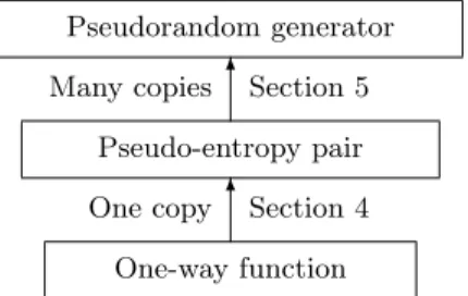
Pseudorandom generator Pseudo-entropy pair One-way function 6Section 4 6Section 5 One copy Many copies
Fig. 1.Overview of our construction.
In this work we explicitly describe an O(n8) construction (in an unrolled version the construction we describe is the one sketched in [6]). Compared to [6]
we choose a different way of presenting this construction; namely we use a two-step approach (see Figure 1). First, (in Section 4) we use the one-way function to construct a pair (g, P) whereg is an efficiently evaluable function andP is a predicate. The pair will satisfy that predictingP(x) fromg(x) is computationally difficult (in particular, more difficult than it would be information theoretically). In [5] the termpseudo-entropy pair is coined for such a pair and we will use this term as well. In a second step we use many instances of such a pseudo-entropy pair to construct a pseudorandom generator.
Further, we generalize the construction to the case where stronger security guarantees on the one-way function are given. This enables us to give more efficient reductions under stronger assumptions.
Indepenently of this work, Haitner, Harnik, and Reingold [5] give a bet-ter method to construct a pseudo-entropy pair from a one-way function. Their construction has the advantage that the entropy ofP(x) giveng(x) can be esti-mated, which makes the construction of the pseudorandom generator from the pseudo-entropy pair more efficient.
3
Definitions and Result
3.1 Definitions and Notation
Definition 1. A one-way function with securitys(n) againstt(n)-bounded in-verters is an efficiently evaluable family of functionsf :{0,1}n → {0,1}m such that for any algorithm running in time at mostt(n)
Pr x←R{0,1}n
[f(A(f(x))) =f(x)]< 1 s(n) for all but finitely manyn.
For example the standard notion of a one-way function is a function which is one-way with securityp(n) against p(n)-bounded inverters for all polynomi-alsp(n).
In [15] it is shown that a random permutation is 2n/10-secure against 2n/5 -bounded inverters, and also other reasons are given why it is not completely unreasonable to assume the existence of one-way permutations with exponential security. In our main theorem we can use one-way functions with exponential security, a weaker primitive than such permutations.
Definition 2. Apseudorandom-generator with securitys(`) againstt(` )-boun-ded distinguishers is an efficiently evaluable family of (expanding) functions h:{0,1}`→ {0,1}`+1 such that for any algorithm running in time at most t(`)
x Pr ←R{0,1}` [A(h(x)) = 1]− Pr u←R{0,1}`+1 [A(u) = 1] ≤ 1 s(`), for all but finitely many`.
The standard notion of a pseudorandom generator is a pseudorandom gen-erator with securityp(`) againstp(`)-bounded distinguishers, for all polynomi-alsp(`).
As mentioned above, we use pseudo-entropy pairs as a step in our construc-tion. For such a pair of functions we first define the advantage an algorithm A has in predictingP(w) fromg(w) (by convention, we use the letterwto denote the input here).
Definition 3. For any algorithm A, any function g : {0,1}n → {0,1}m and any predicateP :{0,1}n→ {0,1}, the advantage ofAin predictingP givengis
AdvA(g, P) := 2 Pr w←R{0,1}n [A(g(w)) =P(w)]−1 2 .
The following definition of a pseudo-entropy pair contains (somewhat surpris-ingly) the conditioned entropy H(P(W)|g(W)); we give an explanation below.
Definition 4. A pseudo-entropy pair with gap φ(n) against t(n)-bounded pre-dictors is a pair (g, P) of efficiently evaluable functions g : {0,1}n → {0,1}m andP :{0,1}n→ {0,1} such that for any algorithmA running in timet(n)
AdvA(g, P)≤1−H(P(W)|g(W))−φ,
for all but finitely manyn(where W is uniformly distributed over {0,1}n). The reader might think that it would be more natural if we used the best advantage for computationally unbounded algorithms (i.e., the information the-oretic advantage), instead of 1−H(P(W)|g(W)). Then φ would be the gap which comes from the use oft(n)-bounded predictors. We quickly explain why we chose the above definition. First, to get an intuition for the expression 1−H(P(W)|g(W)), assume that the pair (g, P) has the additional property that for every inputw, g(w) either fixes P(w) completely or does not give any information about it, i.e., for a fixed value v either H(P(W)|g(W) = v) = 1 or H(P(W)|g(W) = v) = 0 holds. Then, a simple computation shows that 1−H(P(W)|g(W)) is a tight upper bound on the advantage of computationally unbounded algorithms, i.e., in this case our definition coincides with the above “more natural definition”. We mention here that the pairs (g, P) we construct will be close to pairs which have this property. If there are values v such that 0< H(P(W)|g(W) =v)<1, the expression 1−H(P(W)|g(W)) is not an up-per bound anymore and in fact one might achieve significantly greater advantage than 1−H(P(W)|g(W)). Therefore in this case, Definition 4 requires something stronger than the “more natural definition”, and, consequently, constructing a pseudorandom generator from a pseudo-entropy pair becomes easier.1
We use k to denote concatenation of strings,ax denotes the multiplication of bitstrings a and xover GF(2n) (with an arbitrary representation), and x|λ
1
In fact, we do not know a direct way to construct a pseudorandom generator from a pseudo-entropy pair with the “more natural definition”.
denotes the first bλc bits of the bit string x. For fixed x and x, x 6= x, the probability that (ax)|i equals (ax)|i for uniformly chosenacan be computed as
Pr a←{0,1}n (ax)|i = (ax)|i = Pr a←{0,1}n (a(x−x))|i= 0i= 2−i, (1)
an expression we will use later.
For bitstringsxandrof the same lengthnwe usexr:=Lni=1xiri for the inner product. We use the convention thatf−1(y) :=
x∈ {0,1}n|f(x) =y , i.e.,f−1returns a set.
For two distributionsPX0 andPX1 overX the statistical distance is
∆(X0, X1) := 1 2 X x∈X |PX0(x)−PX1(x)|.
We also say that a distribution is ε-close to another distribution if the statis-tical distance of the distributions is at most ε. For a distribution PX over X the min-entropy is H∞(X) := −log(maxx∈XPX(x)). For joint distributions
PXY over X × Y the conditional min-entropy is defined with H∞(X|Y) :=
miny∈YH∞(X|Y =y).
Finally, we define [n] :={1, . . . , n}.
3.2 Result
We give a general construction of a pseudorandom generator from a one-way function. The construction is parametrized by two parametersεandφ. The pa-rameterεshould be chosen such that it is smaller than the target indistinguisha-bility of the pseudorandom generator: an algorithm which distinguishes the out-put of the pseudorandom generator with advantage less thanεwill not help us in inverting f. The second parameter φ should be chosen such that the given one-way function cannot be inverted with probability more than about 2−nφ(as an example, for standard security notions choosing φ= 1n andε = 2−n would be reasonable – these should be considered the canonical choices).
Theorem 1. Let functionsf :{0,1}n → {0,1}m,φ:
N→[0,1],ε:N→[0,1] be given, computable in timepoly(n), and satisfying2−n≤ε≤ 1
n ≤φ.
There exists an efficient to evaluate oracle function hfε,φ with the following properties:
– hfε,φ is expanding,
– hfε,φ has input of lengthO(nφ44log( 1 ε)), and
– an algorithm A which distinguishes the output of hfε,φ from a uniform bit string with advantageγ can be used to get an oracle algorithm which inverts f with probabilityO(n13)2−nφ, usingpoly(n,
1
For example, if we set φ := log(n)/n and ε := n−log(n) = 2−log2(n) and use a standard one-way function in the place of f, thenhfε,φ will be a standard pseudorandom generator, usingO(n8) bits2 of randomness.
Corollary 1. Assume that f : {0,1}n → {0,1}m is a one-way function with security p(n) against p(n)-bounded inverters, for all polynomials p(n). Then there exists a pseudorandom generatorh:{0,1}`→ {0,1}`+1 with security p(`) against p(`)-bounded distinguishers, for all polynomials p(`). The construction calls the one-way function for one fixedndependent of`and satisfies`∈ O(n8). Alternatively if we have a much stronger one-way function which no poly-nomial time algorithm can invert with better probability than 2−cn for some constant c, we can set φto some appropriate small constant andε:=n−log(n), which gives us a pseudorandom generator using O(n4log2
(n)) bits of input:
Corollary 2. Assume that f :{0,1}n→ {0,1}m is a one-way function with se-curity2−cn against p(n)-bounded inverters, for some constantc and all polyno-mials p(n). Then there exists a pseudorandom generator h:{0,1}`→ {0,1}`+1 with security p(`) against p(`)-bounded distinguishers, for all polynomials p(`). The construction calls the one-way function for one fixed ndependent of`, and satisfies`∈ O(n4log2(n)).
If we want a pseudorandom generator with stronger security we setεsmaller in our construction. For example, if a one-way functionf has security 2cnagainst 2cn bounded distinguishers, we set φ (again) to an appropriate constant and ε:= 2−n. With these parameters our construction needsO(n5) input bits, and, for an appropriate constantd, an algorithm with distinguishing advantage 2−dn, and running in time 2dn, can be used to get an inverting algorithm which con-tradicts the assumption aboutf. (A corollary similar to the ones before could be formulated here).
The proof of Theorem 1 is in two steps (see Figure 1). In Section 4 we use the Goldreich-Levin Theorem and two-universal hash-functions to obtain a pseudo-entropy pair. In Section 5 we show how such a pair can be used to obtain a pseudorandom generator.
3.3 Extractors
Informally, an extractor is a function which can extract a uniform bit string from a random string with sufficient min-entropy. The following well known left-over hash lemma from [10] shows that multiplication over GF(2n) with a randomly chosen string aand then cutting off an appropriate number of bits can be used to extract randomness. For completeness we give a proof (adapted from [12]).
Lemma 1 (Left-over hash lemma). Let x∈ {0,1}n be chosen according to any source with min-entropyλ. Then, for anyε >0, and uniform randoma, the distribution of (ax)|λ−2 log(1 ε) a is ε
2-close to a uniform bit string of length
bλ−2 log(1ε)c+n.
2
Proof. Letm:=bλ−2 log(1
ε)c, andPV Abe the distribution of (ax)|mka. Further, letPU be the uniform distribution over{0,1}m+n. Using the Cauchy-Schwartz inequality (Pki=1ai)2≤k
Pk i=1a
2
i we obtain for the statistical distance in ques-tion ∆(V A, U) = 1 2 X v∈{0,1}m,a∈{0,1}n PV A(v, a)− 1 2n2m ≤ 1 2 √ 2n2m v u u t X v,a P2 V A(v, a)−2 X v,a PV A(v, a) 2n2m + X v,a 1 2n2m 2 = 1 2 √ 2n2m s X v,a P2 V A(v, a)− 1 2n2m. (2)
Let now X0 and X1 be independently distributed according to PX (i.e., the source with min-entropyλ). Further, letA0andA1be independent over{0,1}n. The collision probability of the output distribution is
Prh (X0A0)|m A0= (X1A1)|m A1 i =X v,a PV A2 (v, a).
Thus we see that equation (2) gives an un upper bound on∆(V A, U) in terms of the collision probability of two independent invocations of the hash-function on two independent samples from the distribution PX. We can estimate this collision probability as follows:
Prh (X0A0)|m A0 = (X1A1)|m A1 i = Pr[A0=A1] Pr[(X0A0)|m= (X1A0)|m] ≤Pr[A0=A1] Pr[X0=X1] + Pr h (X0A0)|m= (X1A0)|m X06=X1 i ≤ 1 2n 1 2m+2 log(1/ε)+ 1 2m =1 +ε 2 2n2m, (3)
where we used (1) in the last inequality. We now insert (3) into (2) and get ∆(V A, U)≤ ε
2. ut
Using the usual definition of an extractor, the above lemma states that mul-tiplying with a random element of GF(2n) and then cutting off the last bits is a strong extractor. Consequently, we will sometimes use the notation Extm(x, a) to denote the function Extm(x, a) := (ax)|m
a, extractingbmcbits from x. Further we use the following proposition on independent repetitions from [8], which is a quantitative version of the statement that for k independent repetitions of random variables, the min-entropy of the resulting concatenation is roughlyktimes the (Shannon-)entropy of a single instance (assumingklarge enough and tolerating a small probability that something improbable occured). A similar lemma with slightly weaker parameters is given in [10] (the latter would be sufficient for our application, but the expression from [8] is easier to use).
Proposition 1. Let (X1, Y1), . . . ,(Xk, Yk) i.i.d. according to PXY. For any ε there exists a distribution PX Y which has statistical distance at most 2ε from (X1, . . . , Xk, Y1, . . . , Yk)and satisfies
H∞(X|Y)≥kH(X|Y)−6
p
klog(1/ε) log(|X |).
We can combine the above propositions as follows:
Lemma 2. Let k,εwithk >log(1/ε)be given. Let(X1, Y1), . . . ,(Xk, Yk)i.i.d. according toPXY overX × Y withX ⊆ {0,1}n. LetAbe uniform over{0,1}kn.
Then, Ext kH(X|Y)−8 log(|X |) √ klog(1/ε) X1k · · · kXk, A kY1k · · · kYk
is ε-close to U ×Yk, where U is an independent uniform chosen bitstring of lengthbkH(X|Y)−8 log(|X |)pklog(1/ε)c+kn.
Proof. Combine Lemma 1 and Proposition 1. ut
4
A Pseudo-entropy Pair from any One-way Function
The basic building block we use to get a pseudo-entropy pair is the following theorem by Goldreich and Levin [4] (recall thatxr=x1r1⊕ · · · ⊕xnrnis the inner product ofxandr):
Proposition 2 (Goldreich-Levin). There is an oracle algorithm B(·) such that for anyx∈ {0,1}n and any oracleA satisfying
Pr r←R{0,1}n
[A(r) =xr]≥ 1
2 +γ BAdoesO(n
γ2)queries toAand then efficiently outputs a list ofO( 1
γ2)elements such that xis in the list with probability 1
2.
This proposition implies that for any one-way functionf, no efficient algo-rithm will be able to predict xr from f(x) and r much better than random guessing, as otherwise the one-way function can be broken.
This suggests the following method to get a pseudo-entropy pair: if we define g(x, r) := f(x)kr and P(x, r) := xr, then predictingP(x, r) from g(x, r) is computationally hard. The problem with this approach is that since f(x) may have many different preimages,H(P(X, R)|g(X, R))≈1 is possible. In this case, P(x, r) would not only be computationally unpredictable, but alsoinformation theoretically unpredictable, and thus (g, P) will not be a pseudo-entropy pair.
The solution of this problem (as given in [6]), is that one additionally ex-tracts some information of the input x to f; the amount of information ex-tracted is also random. The idea is that in case one is lucky and extracts roughly
log f−1(f(x))
bits, then these extracted bits and f(x) fix xin an informa-tion theoretic way, but computainforma-tionally xr is still hard to predict because of Proposition 2.
Thus, we define functionsg:{0,1}4n → {0,1}m+4nandP :{0,1}4n→ {0,1} as follows (wherei∈[n] is a number3,x,a, and rare bitstrings, and we ignore padding which should be used to get (ax)|i to lengthn)
g(x, i, a, r) :=f(x)i a (ax)|i r (4) P(x, i, a, r) :=xr. (5)
We will alternatively write g(w) and P(w), i.e., we use w as an abbreviation for (x, i, a, r). We will prove that (g, P) is a pseudo-entropy pair in case f is a one-way function. Thus we show that no algorithm exceeds advantage 1−
H(P(W)|g(W))−φ in predictingP(w) fromg(w) (the gapφdoes not appear in the construction, but the pair will have a bigger gap if the one-way function satisfies as stronger security requirement, as we will see).
We first give an estimate onH(P(W)|g(W)). The idea is that we can distin-guish two cases: eitheri≥log(|f−1(f(x))|), in which caseH(P(W)|g(W))≈0, since (ax)|i, a, and f(x) roughly fix x, ori < log(|f−1(f(x))|), in which case H(P(W)|g(W))≈1.
Lemma 3. For the functions g andP as defined above H(P(W)|g(W))≤ Ex←R{0,1}n[log(|f
−1(f(x))|)] + 2 n
Proof. From (1) and the union bound we see that ifi >log(|f−1(y)|) the prob-ability thatxis not determined by the output ofgis at most 2−(i−log(|f−1(y)|)). This impliesH(P(W)|g(W), f(X) =y, I =i)≤2−(i−log(|f−1(y)|)), and thus
H(P(W)|g(W)) = 1 2n X x∈{0,1}n H P(W)|g(W), f(X) =f(x) = 1 2n X x∈{0,1}n 1 n n X i=1 H P(W)|g(W), f(X) =f(x), I=i ≤ 1 2n X x∈{0,1}n log(|f−1(f(x))|) n +1 n n X i=dlog(|f−1(f(x))|)e 2−(i−log(|f−1(f(x))|)) ! ≤ 1 2n X x∈{0,1}n log(|f−1(f(x))|) + 2 n 3
Technically, we should chooseias a uniform number from [n]. We can use annbit string to choose a uniform number from [2n] and from this we can get an “almost”
uniform number from [n] (for example by computing the remainder when dividing byn). This only gives an exponentially small error which we ignore from now on.
= Ex←R{0,1}n[log(|f
−1(f(x))|)] + 2
n .
u t
We can now show that (g, P) is a pseudo-entropy pair. For this, we show that any algorithm which predicts P from g with sufficient probability can be used to invertf. Recall thatφis usually 1n.
Lemma 4. Let f : {0,1}n → {0,1}m and φ :
N → [0,1] be computable in timepoly(n). Let functions g andP be as defined above. There exists an oracle algorithm B(·) such that, for anyA which has advantage AdvA(gf, Pf) ≥1−
H(Pf(W)|gf(W))−φin predicting Pf from gf,BA inverts f with probability Ω( 1
n3)2
−nφandO(n3)calls to A.
We find it convenient to present our proof using random experiments called “games”, similar to the method presented in [14].
Proof. Assume that a given algorithmA(y, i, a, z, r) has an advantage exceeding the bound in the lemma in predictingPfromg. To invert a given inputy=f(x), we will choose i, a, and z uniformly at random. Then we run the Goldreich-Levin algorithm usingA(y, i, a, z,·), i.e., the Goldreich-Levin callsA(y, i, a, z, r) for many different r, but always using the same y, i, a, and z. This gives us a list L containing elements from {0,1}n. For every x ∈ L we check whether f(x) =y. If at least onex∈Lsatisfies this we succeeded in invertingf.
In order to see whether this approach is successful, we first define αto be the advantage ofAfor a fixedy,i,aandzin predictingxrfor a preimagex ofy: α(y, i, a, z) := max x∈f−1(y) 2 Pr r←{0,1}n[A(y, i, a, z, r) =xr]−1 .
We maximize over all possible x ∈ f−1(y), since it is sufficient if the above method findsanypreimage ofy. We will set the parameters of the algorithm such that it succeeds with probability 1
2 if α(y, i, a, z)> 1
4n (i.e., with probability 1 2 the list returned by the algorithm contains x). It is thus sufficient to show for uniformly chosen x, i, a, and z the inequality α(f(x), i, a, z) > 4n1 is satisfied with probability Ω(n13)2
−nφ.
Together with Lemma 3, the requirement of this lemma implies that in the following Game 0 the expectation of the output is at least 1−H(Pf(W)|gf(W))−
φ≥1−1
nEx[log(|f
−1(f(x))|)]−2
n−φ(this holds evenwithoutthe maximization in the definition ofαand usingx=xinstead – clearly, the maximization cannot reduce the expected output of Game 0).
Game 0:
x←R{0,1}n,y:=f(x),i←R[n] a←R{0,1}n,z:= (ax)|i
Note that even though we can approximateα(y, i, a, z) we do not know how to compute the exact value in reasonable time. However, we do not worry about finding an efficient implementation of our games.
Ifiis much larger than log(|f−1(y)|) then predictingP(w) fromg(w) is not very useful in order to invert f, since (ax)|i gives much information about x which we do not have if we try to inverty. Thus, we ignore the cases whereiis much larger than log(|f−1(y)|) in Game 1.
Game 1: x←R{0,1}n,y:=f(x),i←R[n] if i≤log(|f−1(y)|) +nφ+ 3then a←R{0,1}n, z:= (ax)|i outputα(y, i, a, z) fi output0
It is not so hard to see that the probability that the if clause fails is at most 1−1
nEx[log(|f
−1(f(x))|)]−3
n−φ. Thus, in Game 1 the expectation of the output is at least 1
n (because the output only decreases in case the if clause fails, and in this case by at most one).
In Game 2, we only choose the firstj bits of z as above, where j is chosen such that these bits will be 4n1-close to uniform (this will be used later). We fill up the rest of z with the best possible choice; clearly, this cannot decrease the expectation of the output.
Game 2:
x←R{0,1}n,y:=f(x),i←R[n]
if i≤log(|f−1(y)|) +nφ+ 3then
j:= min(blog(|f−1(y)|)−2 log(4n)c, i) a←R{0,1}n, z1:= (ax)|j
set z2∈ {0,1}j−i such thatα(y, i, a, z1kz2) is maximal
outputα(y, i, a, z1kz2)
fi output0
We now chosez1 uniformly at random. Lemma 1 implies that the statistical distance of the previous distribution ofz1to the uniform distribution (givena,i, andybut notx) is at most 4n1. Thus, the expecation of the output is at least 2n1 .
Game 3:
x←R{0,1}n,y:=f(x),i←R[n]
if i≤log(|f−1(y)|) +nφ+ 3then j:= min(blog(|f−1(y)|)−2 log(4n)c, i) a←R{0,1}n, z1←R{0,1}j
set z2∈ {0,1}j−i such thatα(y, i, a, z1kz2) is maximal
outputα(y, i, a, z1kz2)
fi output0
As mentioned above, we will be satisfied if we have valuesy, i, a,(z1kz2) such that α(y, i, a, z1kz2)≥4n1. In Game 4, we thus do not compute the expectation ofαanymore, but only outputsuccessif this is satisfied, andfailotherwise.
Game 4:
x←R{0,1}n,y:=f(x),i←R[n]
if i≤log(|f−1(y)|) +nφ+ 3then
j:= min(blog(|f−1(y)|)−2 log(4n)c, i) a←R{0,1}n, z1←R{0,1}j
set z2∈ {0,1}j−i such thatα(y, i, a, z1kz2) is maximal
if α(y, i, a, z1kz2)> 4n1
outputsuccess
fi fi
outputfail
The usual Markov style argument shows that the probability that the output is successis at least 1
4n (this is easiest seen by assuming otherwise and computing an upper bound on the expectation of the output in Game 3: it would be less than 1
2n).
In Game 5, we choose all ofz uniformly at random.
Game 5: x←R{0,1}n,y:=f(x),i←R[n] if i≤log(|f−1(y)|) +nφ+ 3then a←R{0,1}n, z←R{0,1}i if α(y, i, a, z)> 1 4n outputsuccess fi fi outputfail
In Game 5, we can assume thatzis still chosen asz1kz2. Forz1, the distribution is the same as in Game 4, forz2, we hope that we are lucky and choose it exactly as in Game 4. The length ofz2is at most 2 log(4n)+nφ+3, and thus this happens with probability at least 128n1 22−
nφ. Thus, in Game 4, with probability at least 1
512n32−
nφthe output issuccess. As mentioned at the start of the proof, in this case running the Goldreich-Levin algorithm with parameter 1
4n will invert f with probability 1
2, which means that in total we have probabilityΩ( 1 n3)2
−nφin
invertingf. ut
5
A Pseudorandom Generator from a Pseudo-entropy
Pair
We now show how we can obtain a pseudorandom generator from a pseudo-entropy pair (g, P) as constructed in the last section. The idea here is that we use many (sayk) parallel copies of the functiong. We can then extract about
kH(g(W)) bits from the concatenated outputs ofg, about kH(W|g(W)P(W)) bits from the concatenated inputs, and aboutk(H(P(W)|g(W)) +φ) bits from the concatenated outputs ofP. Using the identityH(g(W)) +H(P(W)|g(W)) + H(W|g(W)P(W)) =H(W), we can see that this will be expanding, and we can say that thekφbits of pseudorandomness fromP are used to get the expanding property ofh.
The key lemma in order to prove the security of the construction is the following variant of Impagliazzo’s hard-core lemma [9] proven in [7]4. For a set
T letχT be the characteristic function ofT:
χT(x) :=
(
1 x∈ T
0 x /∈ T .
Proposition 3 (Uniform Hard-Core Lemma).Assume that the given func-tionsg:{0,1}n→ {0,1}m,P :{0,1}n → {0,1},δ:
N→[0,1]andγ:N→[0,1] are computable in timepoly(n), whereδ is noticeable andγ >2−n/3.
Further, assume that there exists an oracle algorithmA(·) such that, for in-finitely many n, the following holds: for any set T ⊆ {0,1}n with |T | ≥ δ2n, AχT outputs a circuitC satisfying
E Pr x←RT
[C(g(x)) =P(x)]≥ 1 +γ
2 (where the expectation is over the randomness of A).
Then, there is an algorithmB which callsAas a black boxpoly(γ1, n)times, such that
AdvB(g, P)≥1−δ
for infinitely many n. The runtime of B is bounded by poly(1
γ, n) times the runtime ofA.
The advantage of using Proposition 3 is as follows: in order to get a con-tradiction, we will use a given algorithm A as oracle to contradict the hard-ness of a pseudo-entropy pair, i.e., we will giveB such that AdvB(g, P)≥1−
H(P(W)|g(W))−φ. Proposition 3 states that for this it is sufficient to show how to get circuits which perform slightly better than random guessing on a fixed set of size 2n(H(P(W)|g(W)) +φ), given access to a description of this set. Often, this is a much simpler task.
In the following construction of a pseudorandom generator from a pseudo-entropy pair we assume that parametersεand φare provided (thus they reap-pear in Theorem 1). The parameterε describes how much we lose in the indis-tinguishability (by making our extractors imperfect), while φ is the gap of the pseudo-entropy pair.
4 The proposition here is slightly stronger then the corresponding lemma in [7], as we
do not requireγto be noticeable. It is easy to see that the proof in [7] works in this case as well.
Further we assume that parametersα and β are known which give certain information about the combinatorial structure of the given predicate. We will get rid of this assumption later by trying multiple values forαand β such that one of them must be correct.5
Lemma 5. LetgandP be efficiently evaluable functions,g:{0,1}n→ {0,1}m, P : {0,1}n → {0,1}, ε : [0,1] →
N, and φ : [0,1] → N be computable in polynomial time, φ > 1n. Assume that parametersαandβ are such that
α≤H(P(W)|g(W))≤α+φ/4 β ≤H(g(W))≤β+φ/4.
There is an efficient to evaluate oracle function hgα,β,ε,φ with the following properties:
– hgα,β,ε,φ is expanding,
– hgα,β,ε,φ has inputs of lengthO(n3 1 φ2log(
1 ε)), and
– any algorithmAwhich distinguishes the output ofhgα,β,ε,φfrom a uniform bit string with advantageγcan be used to get an oracle algorithmBA satisfying AdvB(g, P)≥1−H(P(W)|g(W))−φ which doespoly(γ−1ε, n)calls to A. Proof. Letk:= 4096·(nφ)2·log(3
ε) be the number of repetitions (this is chosen such that kφ 8 = 512 n2 φ log 3 ε = 8n r klog3 ε , (6)
which we use later). To simplify notation we set λ:=n−α−β −φ/2. Using the notation wk :=w
1k. . .kwk, g(k)(wk) :=g(w1)k. . .kg(wk) and P(k)(wk) := P(w1)k. . .kP(wk), the functionhα,β,ε,φis defined as
hα,β,ε,φ(wk, s1, s2, s3) := Extk(β−φ/8) g(k)(wk), s1 Extk(α+7φ/8) P (k)(wk), s 2 Extk(λ−φ/8) w k, s 3 . Clearly, the input length is O(n3 1
φ2log( 1
ε)). We further see by inspection that, excluding the additional randomnesss1,s2, ands3, the functionhmapsknbits to at leastk(α+β+λ) + 5kφ8 −3 =k(n−φ2) +k5φ8 −3 =k(n+φ8)−3> kn bits. Since the additional randomness is also completely contained in the output, hα,β,ε,φis expanding for almost alln.
We now show that an algorithmA which has advantageγ in distinguishing hα,β,ε,φ(wk, s1, s2, s3) from a uniform bit string of the same length can be used to predictP(w) giveng(w) as claimed above. Per definition the probability that the output istruein the following game is at least 1+γ2 .
5
Haitner, Harnik, and Reingold [5] construct a pseudo-entropy pair for which H(P(W)|g(W)) =1
2 is fixed. Because of this, they are able to save a factor ofnin
the seed length under standard assumptions (they do not need to try different values forα).
Game 0:
(w1, . . . , wk)←R{0,1}nk b←R{0,1}
if b= 0 then (Run Awith the output of h) s1←R{0,1}mk,v1:= Extk(β−φ/8) g(k)(wk), s1
s2←R{0,1}k,v2:= Extk(α+7φ/8) P(k)(wk), s2 s3←R{0,1}nk,v3:= Extk(λ−φ/8) wk, s3
else (Run Awith uniform randomness) v1←R{0,1}mk+k(β−φ/8)
v2←R{0,1}k+k(α+7φ/8) v3←R{0,1}nk+k(λ−φ/8)
fi
outputb=A(v1kv2kv3)
We now make two transition based on statistical indistinguishability. First, we replace the last part v3 in theif-clause of Game 0 with uniform random bits. Because H(W|g(W)P(W)) = H(W)−H(g(W))−H(P(W)|g(W)) ≥ n−
α−β − φ2 = λ, Lemma 2 implies that conditioned on the output of g(k) and P(k) (and thus also conditioned on the extracted bits of those outputs) Extkλ−kφ/8(wk, s3) = Extkλ−8n·√klog(3
ε)
(wk, s3) is ε3-close to the uniform dis-tribution (here we used (6)). Thus this only loses ε/3 of the advantage γ in distinguishing.
Second, we replacev1in theelse-clause with Extk(β−φ/8)(g(k)(wk), s1). Since H(g(W))≥β, Lemma 2 implies that we only loseε/3 in the advantage again. In total, in the following Game 1 we have advantage at leastγ−2ε/3 over random guessing. Game 1: (w1, . . . , wk)←R{0,1}nk b←R{0,1} if b= 0 then s1←R{0,1}mk,v1:= Extk(β−φ/8) g(k)(wk), s1 s2←R{0,1}k,v2:= Extk(α+7φ/8) P(k)(wk), s2 v3←R{0,1}nk+k(λ−φ/8) else s1←R{0,1}mk,v1:= Extk(β−φ/8) g(k)(wk), s1 v2←R{0,1}k+k(α+7φ/8) v3←R{0,1}nk+k(λ−φ/8) fi outputb=A(v1kv2kv3)
We would like to ignore the parts which are the same in caseb = 0 and b= 1. It is easy to see thatA0 in Game 2 can be designed such that it callsAwith the same distribution as in Game 1.
Game 2: (w1, . . . , wk)←R{0,1}nk b←R{0,1} if b= 0 then s←R{0,1}k, v:= Extk(α+7φ/8) P(k)(wk), s else v←R{0,1}k+k(α+7φ/8) fi outputb=A0(g(k)(wk)kv)
Later we want to use Proposition 3. Thus we will have an oracleχT which
implements the characteristic function of a setT of size at least (α+φ)2n. From now on we will use the oracle implicitly in the games by testing whetherw∈ T. In Game 3 it is easy to check that in caseb= 0 the distribution with whichA0 is called does not change from Game 2. On the other hand, ifb= 1, then (since
|T | ≥2n(α+φ)) thep
i contain independent random variables with entropy at leastα+φ(where the entropy is conditioned ong(wi)). Using Lemma 2 we see that in this casevis 3ε-close to uniform, implying that in Game 3 the advantage ofA0 in predictingbis stillγ−ε. Game 3: (w1, . . . , wk)←R{0,1}nk b←R{0,1} for i∈[n]do if wi∈ T ∧b= 1 then pi←R{0,1} else pi:=P(wi) fi od s←R{0,1}k,v:= Extk(α+7φ/8) pk, s outputb=A0(g(k)(w(k))kv)
From Game 3, we will now apply a standard hybrid argument to get a pre-dictor for a single position. For this, consider Game 4.
Game 4: (w1, . . . , wk)←R{0,1}nk j←R[n] for i∈ {1, . . . , j−1}do if wi∈ T thenpi ←R{0,1} elsepi:=P(wi)fi od for i∈ {j+ 1, . . . , n} dopi :=P(wi)od b←R{0,1} if wj ∈ T ∧b= 1thenpj←R{0,1}else pj :=P(wj)fi s←R{0,1}k,v:= Extk(α+7φ/8) pk, s outputb=A0(g(k)(w(k))kv)
The distributionA0 is called in Game 4 in caseb= 0 andj = 1 is the same as in Game 3 in case b= 0; the distribution used in Game 4 in case b= 1 andj =n is the same as in Game 3, in case b = 1. Further, the distribution in Game 4 does not change if b is set from 1 to 0 andj is increased by one. This implies that the advantage ofA0 in predictingb is (γ−ε)/k.
In Game 5, we replaceA0 withA00which does all the operations common in case b= 0 and b = 1 (thew chosen in Game 5 corresponds to wj in Game 4, andA00 chooses the value ofj, and all otherwi before calling A0).
Game 5: w←R{0,1}n b←R{0,1} if w∈ T ∧b= 1then p←R{0,1} outputA00(g(w)kp) =b else outputA00(g(w)kP(w)) =b fi
An easy calculation now yields that forw←RT andp←R{0,1}the probabillity that
1⊕p⊕A00(g(w)kp) =P(w)
is at least 12+γ−kε. Since this works for anyT with|T | ≥(α+φ)2n, and thus for everyT with|T | ≥(H(P(W)|g(W)) +φ)2n, we can apply Proposition 3 and
get the lemma. ut
With this lemma, we can now prove Theorem 1.
Proof (of Theorem 1). Given εand φ, we use the construction of Lemma 4 to get a predicate which we use in the construction of Lemma 5 for 16nφ2 differ-ent values of α and β (note that 0 ≤ H(g(W)) ≤ n), such that for at least one of those choices the requirements of Lemma 5 hold. Further, in those ap-plications we use ε0 := Ω(εnφ54) in place of ε. Since ε0 = Ω(ε
10), this satisfies
O(log(1ε)) =O(log(ε10)).
For every choice of α and β we concatenate hα,β,ε0,φ : {0,1}` → {0,1}`+1
with itself, in order to obtain a functionh0
α,β,ε0,φ:{0,1}`→ {0,1}16nφ −2`+1
, i.e., the first part of the output of hα,β,ε0,φ is used to call hα,β,ε0,φ again, and this
process is repeated 16nφ−2`∈ O(n5 1
φ4) times, and every time we get one more bit of the final output.
The functionhε,φ :{0,1}16nφ
−2`
→ {0,1}16nφ−2`+1
divides its input into 16nφ2 blocks of length`, calls the functions h0α,β,ε0,φ with seperate blocks, and XORs
the outputs.
Assume now that an algorithm A can distinguish the output of hε,φ from a unifrom random string with advantage γ. For every choice of α and β (and in particular the choice which satisfies the requirements of Lemma 5) we try
the following to invert f. First, since we can simulate the other instances, we see that we have advantage γ in distinguishing the output of h0α,β,ε0,φ from a
random string. We can use the hybrid argument to get an algorithm which has advantage γ0 :=Ω(γφ4n−5) in distinguishing the output of h
α,β,ε0,φ from a
random string. From Lemma 5 we get an algorithm which predictsPfromgwith advantage at least 1−H(P(W)|g(W))−φ, and the number of calls is bounded by poly(γ0−1ε0, n) = poly(
1
γ−ε, n). Finally, Lemma 4 implies that we can get an inverter with the claimed complexity and success probability. ut
Acknowledgments
I would like to thank Ueli Maurer, Krzysztof Pietrzak, Dominik Raub, Renato Renner, Johan Sj¨odin, and Stefano Tessaro for helpful comments and discussions. Also, I would like to thank the anonymous referees who provided helpful criticism about the presentation of this paper. I was supported by the Swiss National Science Foundation, project no. 200020-103847/1.
References
1. Manuel Blum and Silvio Micali. How to generate cryptographically strong se-quences of pseudo-random bits. Siam Journal on Computation, 13(4):850–864, 1984.
2. Oded Goldreich, Shafi Goldwasser, and Silvio Micali. How to construct random functions. Journal of the ACM, 33(4):792–807, 1986.
3. Oded Goldreich, Hugo Krawczyk, and Michael Luby. On the existence of pseudo-random generators. Siam Journal on Computation, 22(6):1163–1175, 1993. 4. Oded Goldreich and Leonid A. Levin. A hard-core predicate for all one-way
func-tions. InProceedings of the Twenty First Annual ACM Symposium on Theory of Computing, pages 25–32, 1989.
5. Iftach Haitner, Danny Harnik, and Omer Reingold. On the power of the random-ized iterate. Technical Report TR05-135, Electronic Colloquium on Computational Complexity (ECCC), 2005.
6. Johan H˚astad, Russell Impagliazzo, Leonid A. Levin, and Michael Luby. A pseu-dorandom generator from any one-way function. Siam Journal on Computation, 28(4):1364–1396, 1999.
7. Thomas Holenstein. Key agreement from weak bit agreement. InProceedings of the Thirty Seventh Annual ACM Symposium on Theory of Computing, pages 664–673, 2005.
8. Thomas Holenstein and Renato Renner. On the smooth R´enyi entropy of inde-pendently repeated random experiments. In preparation, 2005.
9. Russell Impagliazzo. Hard-core distributions for somewhat hard problems. In
The 36th Annual Symposium on Foundations of Computer Science, pages 538– 545, 1995.
10. Russell Impagliazzo, Leonid A. Levin, and Michael Luby. Pseudo-random gener-ation from one-way functions (extended abstract). InProceedings of the Twenty First Annual ACM Symposium on Theory of Computing, pages 12–24, 1989.
11. Michael Luby and Charles Rackoff. How to construct pseudorandom permutations from pseudorandom functions.Siam Journal on Computation, 17(2):373–386, 1988. 12. Michael Luby and Avi Wigderson. Pairwise independence and derandomiza-tion. Technical Report ICSI TR-95-035, International Computer Science Institute, Berkeley, CA, 1995.
13. Moni Naor. Bit commitment using pseudorandomness. Journal of Cryptology, 4(2):151–158, 1991.
14. Victor Shoup. Sequences of games: a tool for taming complexity in security proofs. Technical Report 332,http://eprint.iacr.org/2004/332, 2004.
15. Hoeteck Wee. On obfuscating point functions. InProceedings of the Thirty Seventh Annual ACM Symposium on Theory of Computing, pages 523–532, 2005.
16. Andrew C. Yao. Theory and applications of trapdoor functions (extended ab-stract). In The 23rd Annual Symposium on Foundations of Computer Science, pages 80–91, 1982.