NULL MODEL ANALYSIS OF SPECIES NESTEDNESS PATTERNS
WERNERULRICH1,3ANDNICHOLASJ. GOTELLI21Nicolaus Copernicus University in Torun´, Department of Animal Ecology, Gagarina 9, 87-100 Torun´, Poland 2
Department of Biology, University of Vermont, Burlington, Vermont 05405 USA
Abstract. Nestedness is a common biogeographic pattern in which small communities form proper subsets of large communities. However, the detection of nestedness in binary presence–absence matrices will be affected by both the metric used to quantify nestedness and the reference null distribution. In this study, we assessed the statistical performance of eight nestedness metrics and six null model algorithms. The metrics and algorithms were tested against a benchmark set of 200 random matrices and 200 nested matrices that were created by passive sampling. Many algorithms that have been used in nestedness studies are vulnerable to type I errors (falsely rejecting a true null hypothesis). The best-performing algorithm maintains fixed row and fixed column totals, but it is conservative and may not always detect nestedness when it is present. Among the eight indices, the popular matrix temperature metric did not have good statistical properties. Instead, the Brualdi and Sanderson discrepancy index and Cutler’s index of unexpected presences performed best. When used with the fixed-fixed algorithm, these indices provide a conservative test for nestedness. Although previous studies have revealed a high frequency of nestedness, a reanalysis of 288 empirical matrices suggests that the true frequency of nested matrices is between 10%and 40%.
Key words: biogeography; matrix temperature; nestedness; nestedness temperature calculator; null model; passive sampling; presence–absence matrix; statistical test.
INTRODUCTION
A common biogeographic pattern is species nested-ness: smaller communities form proper subsets of larger communities (Patterson and Atmar 1986, Atmar and Patterson 1993). In an ordered binary presence–absence matrix, nestedness leads to a maximally ‘‘packed’’ pattern of ones and zeroes. Unexpected presences or absences from a maximally packed matrix can be used to quantify the extent of nestedness, both for the matrix as a whole and for individual species (Atmar and Patterson 1993).
Although Darlington (1957) first described the pattern of nestedness and its possible causes, the study of nestedness was popularized by the pioneering work of Patterson and Atmar (1986). These authors compiled published matrices, developed convenient software (the nestedness temperature calculator, NTC), and intro-duced an appealing index of matrix temperature to quantify nestedness (Atmar and Patterson 1993, 1995). The matrix temperature metric uses the Euclidian distances of unexpected empty or filled cells from the isocline that separates presences from absences in a perfectly nested matrix. The sum of these distances is rescaled relative to the maximum possible value for a given matrix size and fill. Using the NTC, Wright et al. (1998) found a large percentage of the matrices compiled
by Atmar and Pattterson (1995) were nested and argued that selective extinction and ordered collapse of com-munities were the primary causes of nested patterns. However, subsequent analyses have revealed potential problems with the NTC and the index of matrix temperature. Wright et al. (1998) found that the matrix temperature index is sensitive to matrix size. Fischer and Lindenmayer (2002) and Higgins et al. (2006) showed that the randomization procedure of NTC is prone to identify nestedness as an artifact of passive sampling. Greve and Chown (2006) found that endemicitiy biases the tests and causes the analyses to incorrectly identify nestedness after the addition of non-nested endemic species to the matrix.
Moreover, high frequencies of mutual species exclu-sions (checkerboards) or pronounced classes of ubiqui-tous and infrequent species (a core-satellite pattern) may cause unstable results or inflated type I error rates (Fischer and Lindenmayer 2002, Rodrı´guez-Girone´s and Santamarı´a 2006). The nearly exclusive use of the matrix temperature measure has given the impression that it is the only index of the degree of nestedness. However, Patterson and Atmar (1986), Cutler (1991), Wright and Reeves (1992), and Brualdi and Sanderson (1999) proposed other measures of nestedness that are based on simple counts of unexpected presences and/or absences. The statistical properties of these indices have not been well-studied, but they do appear to be sensitive to matrix size when used with null model algorithms that include equiprobable row or column constraints (Wright et al. 1998). In contrast, null models that use fixed row Manuscript received 17 July 2006; revised 29 November
2006; accepted 4 December 2006. Corresponding Editor: M. Holyoak.
3E-mail: [email protected]
and column totals (and thus retain more of the structure of the original matrix) may be less sensitive to matrix size, but may also have less power to detect nestedness (Cook and Quinn 1998).
The statistical significance of any nestedness index value has to be tested against some null hypothesis. The respective null distributions are obtained from null models that generate expected index values and the associated confidence limits. Before large meta-analyses are conducted with empirical data sets, it is therefore important to understand the statistical properties of the different indices and null model algorithms (Gotelli 2001). There are two goals of the current study: (1) to systematically analyze the performance of eight nested-ness indices, crossed with six null model algorithms, and two matrix structure types; (2) to re-evaluate the pattern of nestedness in the original collection of published matrices that were compiled by Atmar and Patterson (1995).
MATERIALS ANDMETHODS
We used two types of random presence–absence matrices (200 matrices each) to study the properties of six randomization algorithms and eight measures of nestedness.
Matrix structures
Nested matrices.—Two hundred nested matrices (MN set) were created by randomly sampling individuals from a metacommunity in which population sizes of the species were distributed according to a lognormal species rank order distribution:
S¼S0e½aðRR0Þ 2
ð1Þ in whichSis the number of species per log2(abundance classR),S0is the number of species in the modal class
R0, andais the shape-generating parameter.
Individuals were randomly sampled until a predefined number of species per site was achieved. For each matrix, the shape-generating parameterawas sampled randomly from a uniform distribution between 0.1 and 0.5 (a canonical lognormal has a¼ 0.2 [May 1975]). Total numbers of speciesmand sitesnper matrix were also sampled from uniform distributions (3m200 and 3 n 50). This sampling protocol produced matrices that should be moderately to strongly nested due to passive sampling (Higgins et al. 2006).
Non-nested matrices.—In the second type of matrix (M0set), species occurrences were again determined by Eq. 1, but species numbers per sitemiwere held nearly constant (randomly takingmi,miþ1, ormi1 species). This second type of matrix by definition should not be nested. Note that if all sites have identical numbers of species, the six nestedness measuresN0,N1, UA, UP, and UT (described inNestedness metrics) are undefined. Empirical matrices.—We also analyzed 288 published presence–absence matrices from the set of 294 matrices that were compiled by Atmar and Patterson (1995) We
excluded six matrices from the Atmar and Patterson (1995) compilation because three of them contained only one row or one column, and three others did not allow for computation of all of the nestedness metrics. Prior to analysis, we transposed matrix rows and columns to match the format used here and in species-co-occurrence and biodiversity analyses (rows ¼ species, columns¼ sites).
Nestedness metrics
We analyzed eight indices that have been proposed to quantify the pattern of nestedness in a presence–absence matrix. For all of these indices except NC, the lower the index value, the stronger the pattern of nestedness.
1)N0is a count of how often a species is absent from a site with greater species richness than the most impoverished site in which it occurs (Patterson and Atmar 1986).
2)N1 is the compliment ofN0and is a count of the number of occurrences of a species at sites with fewer species than the richest site in which it occurs (Cutler 1991).
3) NC is a count of the number of species shared over all pairs of sites (Wright and Reeves 1992). NC is invariant if the column totals of the matrix are fixed, so it was not analyzed with the FF and FE algorithms (described inNull model algorithms).
4) UA is a count of unexpected absences of species from more species-rich sites for which the sum of unexpected absences and presences is minimal (Cutler 1991).
5) UP is a count of unexpected presences of species from more species-poor sites for which the sum of unexpected absences and presences is minimal (Cutler 1991).
6) UT is the sum of deviations from perfect nestedness (UT¼UAþUP [Wright et al. 1998]).
7) BR is a count of the number of discrepancies (absences or presence) that must be erased to produce a perfectly nested matrix (Brualdi and Sanderson 1999).
8) MT is a modified version of the matrix temperature measure of Atmar and Patterson (1993).
The original matrix temperature measure did not strictly define the method for isocline construction and it produced unstable results for matrices rich in checker-boards (Rodrı´guez-Girone´s and Santamarı´a 2006) or endemics (Greve and Chown 2006). Therefore, we modified the matrix temperature measure in three ways. First, we did not exclude totally filled rows and columns as does the NTC to compute the isocline. Because such rows and columns occur frequently in observed pres-ence–absence matrices, exclusion might substantially change matrix dimensions and distort the comparisons between different nestedness metrics.
Second, instead of calculating a curved isocline (as in the NTC), we defined the isocline as two line segments that span from the lower-left corner of the first filled column and the upper-right corner of the first filled row
to the point in the center of the matrix that represents the percentage of matrix fill (Fig. 1). The curved isocline in the NTC approximates these linear isoclines, but crosses them twice.
Third, we excluded from the computation of matrix temperature those matrix cells that fell directly on the isocline. If presences or absences close to the isocline are more probable than those that are distant from the isocline, cells directly at the boundary between the filled and the empty parts of the matrix should simply reflect Poisson errors. Their presence might contribute to noise in the matrix, making it more difficult to detect nestedness when it is present. Exclusion of these points also seems appropriate because of small differences that might arise from using linear vs. nonlinear isoclines.
Null model algorithms
We used six null model algorithms to generate randomized matrices. For binary presence–absence matrices, these algorithms reshuffle the values within the matrix, either preserving matrix row or column totals (‘‘fixed’’ algorithms) or allowing row and column totals to vary freely (‘‘equiprobable’’ algorithms). Both types of algorithms retain different amounts of the information contained in the original matrix. The equiprobable algorithms are constrained only by total (matrix-wide) species occurrences. Fixed algorithms additionally constrain species numbers per site or occurrences across sites to match the original matrix. We used the following six algorithms to generate randomized matrices:
1) FF (fixed-fixed) maintains both observed row and column totals (Connor and Simberloff 1979, Gotelli 2000). We implemented this null model with a variation
of the ‘‘sequential swap algorithm’’ (Manly 1995, Gotelli and Entsminger 2001), in which we sequentially reshuffled 5000 randomly sampled 2 32 submatrices that have the same row and column totals after their elements are swapped. Matrices created this way have the same row and column totals as the original matrix. Each subsequent matrix was created with an additional 5000 swaps. The sequential swap algorithm has been extensively studied in the context of species co-occur-rence analyses (Gotelli 2000, Simberloff and Zaman 2000, Miklo´s and Podani 2004, Ulrich 2004). This algorithm has a small bias against finding species segregation patterns (Miklo´s and Podani 2004), but has good statistical properties and performs well on test matrices (Gotelli 2000, Gotelli and Entsminger 2001).
2) FE (fixed row totals, equiprobable column totals) maintains observed row totals but allows column totals to vary randomly. This null model preserves species occurrence frequencies (row totals), but allows species richness per site (column totals) to vary randomly and equiprobably (Gotelli 2000).
3) EF (equiprobable row totals, fixed column totals) maintains observed column totals but allows row totals to vary randomly. This null model preserves species richness per site (column totals), but allows species occurrence frequencies (row totals) to vary randomly and equiprobably (Gotelli 2000). This model was used by Patterson and Atmar (1986) as theirR0model.
4) EE (equiprobable row totals, equiprobable column totals) maintains the total number of species occurrences in the matrix, but allows both row and column totals to vary freely (Gotelli 2000).
5) PE (proportional row totals, equiprobable column totals) maintains column totals, but species are not drawn equiprobably. Instead, species are drawn ran-domly with probabilities set proportional to observed row totals. This model was used by Patterson and Atmar (1986) as theirR1model.
6) LF (lognormal row totals, fixed column totals) maintains column totals, but row totals are determined by a random draw from a lognormal species abundance distribution (Eq. 1).
All null models and nestedness indices were calculated with the software applications Nestedness and Matrix (see Supplement).
Summary statistics
For each combination of null model (six variants), nestedness index (eight indices), and matrix (three matrix types: nested, unnested, empirical), we created 100 null matrices to compare to the observed matrix. Null model distributions appeared to be not significantly skewed. Therefore, we calculated a standardized effect size (SES) as aZ-transformed score (Z¼[xl]/r) to compare the observed index to the distribution of simulated indices (x¼observed index value,l¼mean,
r¼standard deviation of the 100 index values from the simulated matrices). SES values below2.0 or above 2.0 FIG. 1. Matrix temperature isocline construction for a
binary presence–absence matrix. The computation of the distances (dij) of unexpected empty cells (A) and unexpected
filled cells (P) from the isoclines I1and I2 defines the matrix
temperature index. The point F marks the percentage of matrix fill on the matrix diagonal.
indicate approximate statistical significance at the 5% error level (two-tailed test). The SES is derived from meta-analysis (Gurevitch et al. 1992) and can be used to compare results among different matrices and algo-rithms (Gotelli and McCabe 2002).
Diagnostic tests
We used two additional tests to evaluate the statistical behavior of the FF algorithm. First, for the set of nested matrices, we used linear regressions of the SES of each index on matrix shape (the ratiom/n), matrix size (the product m 3n), matrix fill (percentage of 1’s in the matrix), and the difference in species richness of the sites (the quotient of maximum to minimum richness). These analyses reveal the sensitivity of the different nestedness metrics to simple measures of matrix size and shape.
Second, we tested the power of the FF algorithm to detect matrices that are progressively more nested. We began with a set of random matrices created by the EE algorithm and progressively eliminated the unexpected absences and unexpected presences, thus adding more nested structure to the matrix. At each step, we measured the SES for the resulting matrix. Eventually the matrix is completely nested (although note that the fixed-fixed algorithm cannot actually be used for a matrix that is perfectly nested because there are no other matrix rearrangements possible that maintain fixed row and column sums). This analysis reveals how well the algorithm detects pattern is a series of progressively structured matrices. We also conducted the analysis in the other direction, beginning with a perfectly nested matrix and adding more randomness to it. This is a version of the ‘‘noise test’’ introduced by Gotelli et al. (1997), in which random noise is sequentially added to a perfectly ordered matrix.
RESULTS
Non-nested matrices
There were strong differences among the null models in their performance on random matrices. For all of the
nestedness metrics, the fixed-fixed algorithm (FF) gave a random result for approximately 95% of the test cases (lightface, upright type in Table 1). In other words, 95% of the random matrices generated an SES ,j2j, which encompasses approximately 95%of the standard normal distribution. The other algorithms generally failed this criterion, often with substantially inflated type I error rates (boldface type in Table 1). There were a few combinations of algorithm and index that correctly identified null matrices as random in greater than 70%of the cases (italic type in Table 1), but these error rates would still be considered unacceptably high (P,0.30) for conventional hypothesis testing.
Nested matrices
For the nested matrices, a powerful null model and nestedness metric should detect non-randomness at least 50%of the time. In other words, the test should be more likely to reject the null hypothesis than to fail to reject it when the null hypothesis is false and the matrix is actually nested.
By this criterion, the EE, FE, EF, and PE algorithms had good statistical power, and usually rejected the null hypothesis for more than 70%of the matrices (lightface, upright type in Table 2). In contrast, the FF and LF algorithms performed poorly, and usually rejected the null hypothesis less than 25%of the time, even though the set of test matrices was non-random and contained nested structure (boldface type in Table 2).
For both nested and non-nested matrices, the differences among the eight nestedness metrics were less marked than the differences among the six null model algorithms. For the nested matrices, the FF algorithm (fixed row and column sums) and theN1metric (species absences) detected nestedness in 41% of the nested matrices (italic type in Table 2), which was substantially higher for this algorithm than the other nestedness metrics. However, even with this combination, there would still be a substantial risk of a type II error TABLE1. Proportion of random matrices (M0set) for which
randomness was correctly detected by the null model analysis (2,SES,2). Null model Nestedness index N0 N1 NC UA UP UT BR MT FF 0.96 0.93 0.95 0.93 0.96 0.96 0.93 EE 0.13 0.13 0.03 0.40 0.42 0.10 0.12 0.26 FE 0.59 0.55 0.66 0.67 0.48 0.77 0.32 EF 0.37 0.36 0.04 0.39 0.42 0.23 0.05 0.08 PE 0.81 0.34 0.31 0.47 0.79 0.35 0.35 0.37 LF 0.66 0.56 0.52 0.75 0.71 0.50 0.48 0.56
Notes:Typeface indicates the proportion of matrices scored as random: boldface,P,0.70; italic, 0.70,P,0.90; lightface roman,P.0.90. Empty cells occur where the score could not be computed. Null model algorithms are described inMaterials and methods: Null model algorithms, and nestedness indices are described inMaterials and Methods: Nestedness matrices.
TABLE 2. Proportion of nested matrices (MNset) for which
nestedness was detected by the null model analysis (SES, 2 for all indices except NC, for which SES.2 indicates nestedness). Null model Nestedness index N0 N1 NC UA UP UT BR MT FF 0.01 0.41 0.22 0.02 0.02 0.02 0.16 EE 0.94 0.96 0.90 0.87 0.78 0.96 0.98 0.94 FE 0.87 0.9 0.8 0.74 0.91 0.89 0.86 EF 0.88 0.93 0.96 0.82 0.7 0.94 0.94 0.91 PE 0.76 0.85 0.91 0.72 0.59 0.84 0.85 0.81 LF 0.02 0.02 0.04 0.01 0.02 0.02 0.03 0.03
Notes:Typeface indicates the proportion of nested matrices detected; boldface,P,0.25; italic, 0.25,P,0. 50; lightface roman,P.0.50. Empty cells occur where the score could not be computed. Null model algorithms are described inMaterials and methods: Null model algorithms, and nestedness indices are described inMaterials and Methods: Nestedness matrices.
(probability of incorrectly accepting the null hypothesis ¼0.59).
Empirical matrices
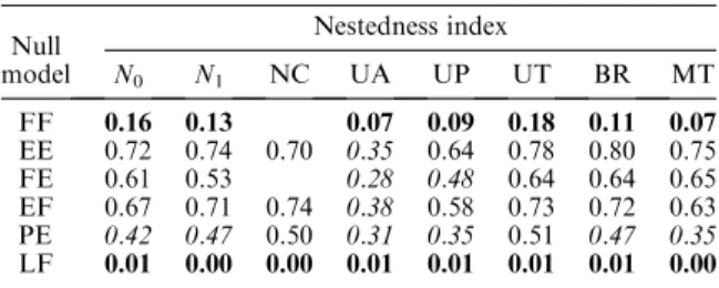
Table 3 gives the frequencies with which nestedness was detected for the 288 empirical matrices compiled by Atmar and Patterson (1995). The proportion of signif-icant matrices varied from a low of 0–1%(all nestedness metrics with the LF algorithm) to a high of 80%(the EE algorithm with the BR nestedness index). The variation in the detection of nestedness mirrored the results of the benchmark tests with random and non-random matri-ces. Namely, conservative algorithms (FF and LF) detected nestedness infrequently (compare with Table 1), whereas liberal algorithms (EE, FE, EF, and PE) detected nestedness frequently (compare with Table 2).
Diagnostic tests
We used the FF null model to test for the behavior of the BR and MT indices during sequential reduction or enhancement of the degree of nestedness. A sequential
elimination of unexpected absences and occurrences in random matrices that were generated by the EE algorithm showed an increase in the number ofZscores ,2 for the BR index (Fig. 2A). Maximally, about 75% of the matrices were correctly identified as being nested. In contrast, MT (matrix temperature) failed to detect nestedness even for the very ordered matrices and identified at most 10% of them as being nested (not shown). The stepwise reduction of the degree of nested-ness starting with an ideally nested matrix resulted for BR in a decrease in the frequency ofZscores,2 until at 50%decrease in nestedness only 6% of the matrices were identified as being nested (Fig. 2B). MT identified 90%of these matrices initially as being disordered (the opposite of nested). With decreasing nestedness, the proportion of matrices identified as being random increased to 90%. The percentage of matrices identified as being nested remained at all steps below 10% (not shown). For the Atmar and Patterson (1995) data set, the BR index identified a maximum of 37% of the matrices as being nested during the stepwise increase in nestedness (Fig. 2C). The MT index identified at most 9%of them as being nested (not shown).
Bivariate correlations using the FF algorithm showed that theZscores of the BR index were least affected by matrix properties (Table 4). Other indices showed significant associations with matrix size, although the signs of the correlations were different. ForN1, UA, and MT, the larger the matrix, the more likely the test would detect nestedness (Fig. 3). However, forN0and UP, the correlation was in the opposite direction, so that nestedness was more likely to be detected in small matrices.
DISCUSSION
Our diagnostic tests clarified the behavior of different null models and different nestedness algorithms, but also complicated the interpretation of empirical nestedness patterns. The analyses of a set of nested and non-nested TABLE 3. Proportion of nested matrices of the Atmar and
Patterson (1995) data set for which nestedness was detected by the null model analysis (SES,2 for all indices except NC, for which SES.2 indicates nestedness).
Null model Nestedness index N0 N1 NC UA UP UT BR MT FF 0.16 0.13 0.07 0.09 0.18 0.11 0.07 EE 0.72 0.74 0.70 0.35 0.64 0.78 0.80 0.75 FE 0.61 0.53 0.28 0.48 0.64 0.64 0.65 EF 0.67 0.71 0.74 0.38 0.58 0.73 0.72 0.63 PE 0.42 0.47 0.50 0.31 0.35 0.51 0.47 0.35 LF 0.01 0.00 0.00 0.01 0.01 0.01 0.01 0.00
Notes:Typeface indicates the proportion of nested matrices detected: boldface,P,0.25; italic, 0.25,P,0.50; lightface roman,P.0.50. Empty cells occur where the score could not be computed. Null model algorithms are described inMaterials and methods: Null model algorithms, and nestedness indices are described inMaterials and Methods: Nestedness matrices.
FIG. 2. Percentage of significantZscores (Z,2) of the BR metric (a count of the number of discrepancies [absences or presence] that must be erased to produce a perfectly nested matrix) under the FF (fixed-fixed) null model (described inMaterials and Methods: Null model algorithms). Three sets of matrices are used in which there is a progressive increase (A, C) or decrease (B) in nestedness. (A) One hundred random matrices (generated by the EE [equiprobable row totals, equiprobable column totals; described inMaterials and Methods: Null model algorithms] algorithm); (B) 100 perfectly nested matrices; (C) 288 empirical matrices compiled by Atmar and Patterson (1995). Note that, in panels A and C, once the 50% increase in nestedness is reached, progressively more matrices became perfectly or nearly perfectly nested. FF is not able to detect nestedness in such cases, and the percentage of significantZscores deceased (not shown).
matrices illustrate the classic trade-off between type I and type II statistical errors. The FF algorithm, in which row and column totals are preserved, has good type I error properties when tested against null matrices (Table 1), but has poor power for detecting nestedness in patterned matrices (Table 2). Because the FF algorithm preserves row and column totals, the observed matrix will more closely resemble matrices created by the FF algorithm than by algorithms that relax row or column totals. This similarity makes it more difficult for the FF algorithm to detect nestedness. Other algorithms, including PE and EF, which were introduced by Patterson and Atmar (1986), have good power to detect nested matrices (Table 2), but are prone to reject the null hypothesis for random matrices (Table 1). For standard statistical tests, guarding against Type I error has traditionally been a high priority (Gotelli and Ellison 2004), so the FF algorithm should be used on these grounds for a conservative test of nestedness. The FF algorithm used with theN1index had the best chance of detecting nested matrices (41%; Table 2).
For this test, 13%of the compiled empirical matrices were significantly nested. Because this is a conservative test, this result represents a lower bound on the true frequency of nestedness in nature. Alternatively, we could use a test that has more power, but at a cost of increased type I error. From the analyses in Table 1 and Table 2, the combination of theN0metric with the PE algorithm has a moderately high type I error frequency (P¼0.19), but comparably good power for detecting nestedness (P ¼ 0.76). By this criterion, 42% of the empirical matrices were nested (Table 3). Thus, the true frequency of nestedness in the empirical matrices is probably between 13% and 42%. This is a substantial fraction, although it is probably lower than the frequencies of 20% (UA index with the EP algorithm) to 70%(NC index with the PE algorithm) reported by Wright et al. (1998) for matrices withP,0.01.
An additional complication is that the N0 and N1 indices appear to be sensitive to matrix size, so that the
probability of detecting nestedness will depend on how large or small the matrix is (Table 4). Wright et al. (1998) reported a similar result for the EE and PE algorithms. With N1 and the FF algorithm, there is a greater chance of detecting nestedness with large matrices than with small. Based on regression of SES against matrix size (Table 4), a nested matrix of at least 340 elements (row number3column number) is needed for an SES of2 (the traditionalP¼0.05 cutpoint). In the Atmar and Patterson (1995) data sets, 138 of the 288 matrices are this size or larger, and of those 20% were significantly nested (SES,2).
Is there a way to distinguish between nestedness patterns caused by passive sampling and nestedness patterns caused by ecologically more relevant mecha-nisms (Andre´n 1994)? Our artificial matrices were generated by passive sampling and the N0, UA, UP, UT, and BR indices identified them with the FF null model as being not nested (Table 2). This raises the question of whether the FF algorithm is generally able to detect nestedness caused by forces other than passive sampling. We used the BR index for this test because it appeared to be least affected by matrix properties (Table 4). We found that the BR index is able to correctly detect and reject nestedness with the FF algorithm for a series of matrices in which we sequentially increased or decreased the degree of nestedness (Fig. 2A, B). In contrast, the BR index did not point to nestedness in the MN matrices (Fig. 2C), which were created by passive sampling.
These analyses suggest that the BR index, used with the FF algorithm, may be able to discriminate between a nested pattern due to passive sampling and nestedness due to other ecological mechanisms. However, matrices constructed by passive sampling may have been less nested than those used in tests that sequentially increased nestedness in the initially random matrices. Moreover, FF tends to retain part of the structure (particularly species numbers and occurrences) of the original matrix (Cook and Quinn 1998). Hence, it might fail to detect nestedness caused by very unequal species numbers and/or site occurrences. For such matrices, other null models that TABLE4. Bivariate Pearson correlation coefficients betweenZ
scores (FF null model) of nestedness measures and matrix shape (the quotient of numbers of rows m to numbers of columnsn), matrix size (m3n), matrix fill (percentage of 1’s in the matrix), and the difference in species richness of the sites (the quotient of maximum to minimum richness). Nestedness index Matrix shape Matrix size Matrix fill Richness difference N0 0.07 0.69*** 0.26 0.43*** N1 0.071* 0.86*** 0.30*** 0.46*** UA 0.14* 0.4*** 0.10 0.23** UP 0.19*** 0.62*** 0.09 0.28** UT 0.09 0.15 0.01 0.09 BR 0.10 0.17 0.03 0.18 MT 0.13 0.27** 0.31*** 0.01
Note:Data are the 200 matrices of the MNdata set, which
were generated by passive sampling. Nestedness indices are described inMaterials and Methods: Nestedness matrices.
*P,0.05; **P,0.01; ***P,0.001.
FIG. 3. The dependence of Zscores of the MT metric (a
modified version of the matrix temperature measure of Atmar and Patterson [1993]) on matrix size (square ofm3n) for the MNmatrices (R2¼0.07,P,0.001).
contain fewer constraints might be more appropriate. Future studies should clarify whether the different biological mechanisms known to produce nested species distributions (Patterson and Atmar 2000) require different null model algorithms and measurements.
In spite of its conceptual appeal, matrix temperature did not perform well as an index for detecting nestedness; the modifications of the MT index that we introduced (calculation of linear isoclines, inclusion of all rows and columns, and exclusion of cells that intercept the isocline) did not improve its performance. With the FF algorithm, the MT index decreased with matrix size and fill (Table 4). This sample-size dependency has also been detected for matrix temperature when used with the EE algorithm (Sfenthourakis et al. 2004, Greve and Chown 2006). From our analyses we conclude that although the concept of matrix temperature was important for popularizing nestedness studies, this index should no longer be used to test for nestedness patterns.
In contrast, the BR index appeared to be largely independent of matrix properties (Table 4). Greve and Chown (2006) reported similarly good statistical prop-erties of BR using the EE algorithm. The reason for this might be that BR links observed and maximally packed matrices in a simple mechanistic way, without making additional assumptions that might be influenced by matrix structure. Although the N1index is sensitive to matrix size, it is not prone to type I errors (Table 1) and has the best power for detecting nested matrices when they are present (Table 2). We suggest, therefore, that the combination of the FF algorithm with the N1 and the BR indices is a conservative test for patterns of nestedness.
Our analyses have clarified the power of different proposed algorithms and metrics to detect patterns of nestedness in binary presence-absence matrices. They focused on the FF algorithm and extend existing tests (Cook and Quinn 1998, Wright et al. 1998) that were based on the EE, EF, and EP algorithms (Table 1). Once nestedness is detected, however, additional analyses may be necessary to distinguish among the hypotheses of selective extinction (Patterson and Atmar 2000, Bruun and Moen 2003), differential dispersal (Cook and Quinn 1995, Loo et al. 2002, McAbendroth et al. 2005), passive sampling (Andre´n 1994, Fischer and Lindenmayer 2002, Higgins et al. 2006), differential habitat quality (Hy-lander et al. 2005), or nesting of habitats (Hausdorf and Hennig 2003, Wethered and Lawes 2005).
ACKNOWLEDGMENTS
This work was supported in part by grants from the Polish Committee for Scientific Research to W. Ulrich (KBN, 3 P04F 034 22, 2 P04F 039 29). N. J. Gotelli was supported by NSF grant 0541936.
LITERATURECITED
Andre´n, H. 1994. Can one use nested subset pattern to reject the random sample hypothesis? Examples from boreal bird communities. Oikos 70:489–491.
Atmar, W., and B. D. Patterson. 1993. The measure of order and disorder in the distribution of species in fragmented habitat. Oecologia 96:373–382.
Atmar, W., and B. D. Patterson. 1995. The nestedness temperature calculator: a visual basic program, including 294 presence absence matrices. AICS Research, Inc., University Park, New Mexico, USA and The Field Museum, Chicago, Illinois, USA.
Brualdi, R. A., and J. G. Sanderson. 1999. Nested species subsets, gaps, and discrepancy. Oecologia 119:256–264. Bruun, H. H., and J. Moen. 2003. Nested communities of alpine
plants on isolated mountains: relative importance of coloni-zation and extinction. Journal of Biogeography 30:297–303. Connor, E. F., and D. Simberloff. 1979. The assembly of species communities: chance or competition? Ecology 60: 1132–1140.
Cook, R. R., and J. F. Quinn. 1995. The influence of colonization in nested species subsets. Oecologia 102:413– 424.
Cook, R. R., and J. F. Quinn. 1998. An evaluation of randomization models for nested species subsets analysis. Oecologia 113:584–592.
Cutler, A. 1991. Nested faunas and extinction in fragmented habitats. Conservation Biology 5:496–505.
Darlington, P. J. 1957. Zoogeography: geographical distribu-tion of animals. Wiley, New York, New York, USA. Fischer, J., and D. B. Lindenmayer. 2002. Treating the
nestedness temperature calculator as a ‘‘black box’’ can lead to false conclusions. Oikos 99:193–199.
Gotelli, N. J. 2000. Null model analysis of species co-occurrence patterns. Ecology 81:2606–2621.
Gotelli, N. J. 2001. Research frontiers in null model analysis. Global Ecology and Biogeography 10:337–343.
Gotelli, N. J., N. J. Buckley, and J. A. Wiens. 1997. Co-occurrence of Australian land birds: Diamond’s assembly rules revisited. Oikos 80:311–324.
Gotelli, N. J., and A. M. Ellison. 2004. A primer of ecological statistics. Sinauer Associates, Sunderland, Massachusetts, USA.
Gotelli, N. J., and G. L. Entsminger. 2001. Swap and fill algorithms in null model analysis: rethinking the Knight’s Tour. Oecologia 129:281–291.
Gotelli, N. J., and D. J. McCabe. 2002. Species co-occurrence: a meta-analysis of J. M. Diamond’s assembly rules model. Ecology 83:2091–2096.
Greve, M., and S. L. Chown. 2006. Endemicity biases nested-ness metrics: a demonstration, explanation and solution. Ecography 29:347–356.
Gurevitch, J., L. L. Morrow, A. Wallace, and J. S. Walsh. 1992. A meta-analysis of field experiments on competition. American Naturalist 140:539–572.
Hausdorf, B., and C. Hennig. 2003. Nestedness of north-west European land snail ranges as a consequence of differential immigration from Pleistocene glacial refuges. Oecologia 135: 102–109.
Higgins, C. L., M. R. Willig, and R. E. Strauss. 2006. The role of stochastic processes in producing nested patterns of species distributions. Oikos 114:159–167.
Hylander, K., C. Nilsson, B. G. Jonsson, and T. Go¨thner. 2005. Differences in habitat quality explain nestedness in a land snail meta-community. Oikos 108:351–361.
Loo, S. E., R. MacNally, and G. P. Quinn. 2002. An experimental examination of colonization as a generator of biotic nestedness. Oecologia 132:118–124.
Manly, B. F. J. 1995. A note on the analysis of species co-occurrences. Ecology 76:1109–1115.
May, R. M. 1975. Patterns of species abundance and diversity. Pages 81–120inM. L. Cody and J. M. Diamond, editors. Ecology and evolution of communities. Belknap, Cambridge, UK.
McAbendroth, L., A. Foggo, D. Rundle, and D. T. Bilton. 2005. Unravelling nestedness and spatial pattern in pond assemblages. Journal of Animal Ecology 74:41–49. Miklo´s, I., and J. Podani. 2004. Randomization of presence–
absence matrices: comments and new algorithms. Ecology 85: 86–92.
Patterson, B. D., and W. Atmar. 1986. Nested subsets and the structure of insular mammalian faunas and archipelagos. Pages 65–82inL. R. Heaney and B. D. Patterson, editors. Island biogeography of mammals. Academic Press, London, UK.
Patterson, B. D., and W. Atmar. 2000. Analyzing species composition in fragments. Bonner Zoologische Monogra-phien 46.
Rodrı´guez-Girone´s, M. A., and L. Santamarı´a. 2006. A new algorithm to calculate the nestedness temperature of pres-ence–absence matrices. Journal of Biogeography 33:924–935. Sfenthourakis, S., S. Giokas, and E. Tzanatos. 2004. From sampling stations to archipelagos: investigating aspects of the
assemblage of insular biota. Global Ecology and Biogeogra-phy 13:23–35.
Simberloff, D., and A. Zaman. 2000. Random binary matrices in biogeographical ecology: Instituting a good neighbor policy. Environmental and Ecological Statistics 9:405–421. Ulrich, W. 2004. Species co-occurrences and neutral models:
reassessing J. M. Diamond’s assembly rules. Oikos 107:603– 609.
Wethered, R., and M. J. Lawes. 2005. Nestedness of bird assemblages in fragmented Afromontane forest: the effect of plantation forestry in the matrix. Biological Conservation 123:125–137.
Wright, D. H., B. D. Patterson, G. M. Mikkelson, A. Cutler, and W. Atmar. 1998. A comparative analysis of nested subset patterns of species composition. Oecologia 113:1–20. Wright, D. H., and J. H. Reeves. 1992. On the meaning and
measurement of nestedness of species assemblages. Oecologia 92:416–428.
SUPPLEMENT