Evolution with Individual and Social Learning in an
Agent-Based Stock Market
Ryuichi YAMAMOTO
Brandeis University
Second Draft
May 30, 2005
Abstract
An agent-based stock market evolves as agents learn from the past experience and adapt their behavior to the evolving market. This paper introduces a learning and adaptation mechanism which allows agents to choose one rule among a set of ideas updated through both individual and social learning. It then examines how the learning mechanism affects the dynamics of the artificial stock market.
1. Introduction
An agent-based stock market consists of a set of interacting heterogeneous agents. The market evolves as agents learn from the past experience and adapt their behavior to the evolving environment. Such learning and adaptive behavior of the agents is usually modeled with approaches of an evolutionary computation. Recent research has shown a variety of computational techniques to describe the evolution in an artificial stock market. One can distinguish the techniques based on at which level the learning of agents is modeled. The previous literature describes learning at either individual or social level. The learning at individual level is usually called “individual learning” where agents update their behavioral rules from their own past performance. The learning at social level is called “social learning” where agents update their rules through directly interacting with other agents. In the previous literature, the level of learning is exogenously given, and agents involve only a particular level of learning when they update their rules. But such a setting doesn’t say anything about why agents choose a particular level of learning to update their trading rules. This paper introduces a learning mechanism which allows agents to choose one rule at each period among a set of ideas updated through both individual and social learning. A trading strategy performed well in the past is more likely to be selected by agents regardless it is created at individual or social level. This framework allows agents to choose a decision rule endogenously among a wider set of ideas. With such evolution, the following two questions are examined.
First, since agents who have a wider set of ideas to choose are more intelligent, a question would arise if the time series from such an economy would move around more closely to a homogeneous rational expectation equilibrium than in an economy with only one level of learning. A convergence property to the rational expectation equilibrium (hereafter REE) is investigated in LeBaron (2000) and Arthur et al. (1996). They find when agents adapt their forecasts very slowly to new observations the market converges to the REE. The more information from the market agents get before updating their rules, the more closely they behave rationally. They deal with such a convergence property by looking at different time-horizon. But this paper investigates a convergence property by looking at different levels of intelligence given a time horizon. Can a market reach the REE if agents have many ideas to process the market information although they adapt their behavior
quickly to new observations? Would agents be able to behave rationally when they are intelligent? However, the result in this paper shows that the economy with more intelligent agents cannot reach the REE. Agents don’t behave rationally when they are intelligent. Intelligent agents are not rational.
The second investigates which level of learning is likely to dominate in the market. This is analyzed by investigating who chooses which level of learning and what proportion of the agents often uses individual or social learning. Agents are allowed to choose endogenously a better idea created from individual and social learning. Some agents with better ideas would use their own idea more often than the others do, while some with less successful ideas would rely on the ideas from other agents. Who has better ideas and who doesn’t? In this paper, it is considered as a better idea that could produce higher wealth over a particular past time span. Agents are more likely to pick an idea which produces higher wealth in the past. So, we would hypothesize that an agent who accumulates more wealth in the past is more likely to pick an idea from her own (from individual learning) than others do, while some who are poor are more likely to adopt an idea from others (from social learning). Then, a question arises what proportion of the agents use their private ideas and imitate others. This paper shows that most of the agents follow the herd, and only agents with very high wealth would possibly rely on private ideas. So, it concludes that the social learning dominates the market. Agents would be better off in an ex ante welfare sense by constraining the use of their own ideas. The second part of the paper eventually indicates that the agent-based stock market in this paper could possibly explain the mechanism of herding behavior in the real world.
The rest of the paper proceeds as follows. Section 2 describes previous literature. Section 3 presents the market structure. Section 4 gives the results from the computer experiments, and the last section concludes.
2. Comparing with Previous Literature
In the previous literature about an agent-based market, a variety of computational techniques are used for evolution in the market. In particular, agents’ trading or forecasting strategies are evolved as agents learn from the past and adapt their behavior to a market. Learning and adaptive behavior of the agents is often described at either individual or
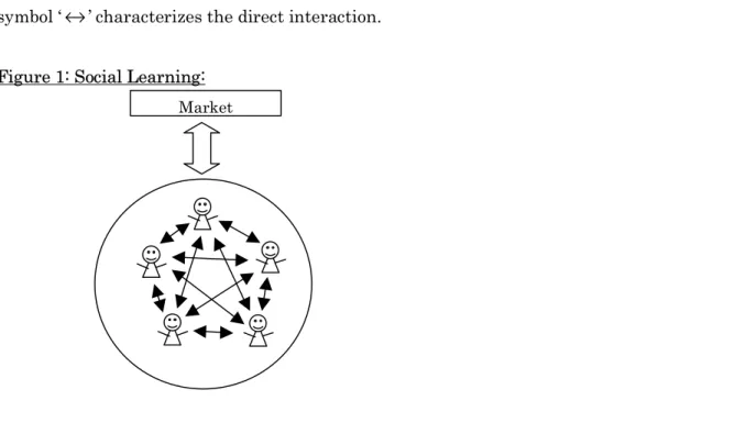
social level. A market with social learning is considered to be a single population consisting of directly interacting heterogeneous agents1 Figure 1 represents a social learning. The symbol ‘
↔
’ characterizes the direct interaction.Figure 1: Social Learning:
In social learning, investors’ behavior is influenced by other investors. Investors meet, for example, at some conferences, communicate each other, and exchange their opinions about the price prediction. Then based on such interactions, they would update their trading strategies.
In a market with individual learning, each agent has a set of her private ideas. The ideas of each agent are not disclosed to other agents so that there is no imitative behavior. Agents learn from their own past experience and update their behavioral rules by themselves. There are no direct exchanges of the ideas among agents in this learning. Reactions to other agents’ behavior only occur indirectly through prices. Figure 2 represents an individual learning. Again, the symbol ‘
↔
’ characterizes the direct interaction, and the symbol ‘=’ shows the indirect interaction. So, in this setting, population indirectly interacts through the market.Mechanisms of learning and adaptive behavior of agents are different in individual and social learning. However, most of the previous papers don’t explain why agents choose
1 Chen et al. (2001) clarifies the distinction between individual and social learnings. Here I follow their
arguments.
a particular level of learning mechanism to update their trading rules. For example, papers Figure 2: Individual Learning
related to the Santa Fe Artificial Stock Market Model adopt an individual learning.2 Some papers allow direct interaction among agents which is represented as social learning.3 Only Vriend (2000) and Yeh and Chen (2000) are the papers which clarify the distinction. Only Yeh and Chen (2000) motivates why agents choose a particular level of learning.
Vriend (2000) compares the simulation results of a simple Cournot model with individual learning and social learning through the same identical genetic algorithm (hereafter GA) for exactly the same identical underlying economic model. The result shows that the difference is essential. For example, the GA with individual learning moves close to the Cournot-Nash output level, whereas the GA with social learning converges to the competitive Walrasian output level. In addition, the social learning GA shows quicker convergence to an equilibrium than the individual learning GA does while the social learning GA reaches higher output levels than the individual learning GA does. So, since the results differ according to the different learning, his result indicates that the choice of the computational modeling between individual and social learning algorithms should be made carefully. Vriend clarifies the distinction but doesn’t mention why and under what condition agents choose a particular level of learning.
Yeh and Chen (2000) construct an artificial stock market which integrates both social learning and individual learning with the genetic programming (GP) framework.
2 These papers include LeBaron, Arthur, and Palmer (1999), Tay and Linn (2001), Arthur, Holland,
Lebaron, Palmer, and Tayler (1996), LeBaron (2001), LeBaron (2002b).
3 Those papers include Arifovic (1996), Arifovic and Gencay (2000), Arifovic (2001a), Arifovic (2001b), and
Arifovic (2002). However, Vriend (2000) and Yeh and Chen (2000) concern the difference of the levels of learning.
Since agents in their market have more ideas to create trading strategies than the single population GP based market, they ask how the degree of traders’ intelligence influences the economy. In particular, first, the econometric properties of time series are examined under different degrees of intelligence. Second, their experiment examines which types of traders are more likely to survive between prediction accuracy and profit oriented traders. Their results show that profit oriented traders are more adaptive and easier to survive while they don’t get much difference of the time series properties in different levels of intelligence. Their paper is the only one which clarifies the distinction between individual and social learning and why agents choose a particular level of learning.
This paper differs on some points from each of the above two papers. First, this paper concerns a model of stock market while Vriend (2000) deals with a Cournot model. Second, although Yeh and Chen (2000) integrate individual and social learning into one model, the agents choose ideas produced either from individual or social learning. Agents select an idea after they go to either level of learning. So, at each stage of decision-making, each agent is allowed to pick one idea only from a particular level of learning. But this paper allows agents to choose one idea from a set of ideas updated from both levels of learning. Each agent has her own ideas and updates them in her mind while she has a set of ideas which evolve with other agents. At a time of decision making, she refers to a set of ideas evolved at individual and social levels.
The second experiment of this paper considers more intelligent agents. Then what would happen to the time series from such an economy? Does it move around more closely to the REE than in an economy with only one level of learning. This investigation differs from works of LeBaron (2000) and Arthur et al. (1996). They deal with the REE property by looking at different time-horizon, and conclude that a market with more observations about the prices can converge to the REE. But this paper asks the convergence property with more intelligent economy.
The last part of the second experiment investigates which level of learning dominates the market, and shows that most of the agents often follow the herd, and only small portion of agents with very high wealth are more likely to use private ideas. This conclusion is consistent with the herding literature4 and the evidence in the actual stock market (Graham (1999)).
3. Market Structure
This section describes an artificial stock market based on the one outlined in LeBaron et al. (1999). In the following sections, the experiments are conducted on an artificial stock market with different styles of learning. But the market structure is exactly identical for all experiments. It is presented as follows.
The artificial stock market has two tradable assets, a risky stock and risk free bond. The risk-free bond is in infinite supply and it pays a constant interest rate,
r
f =10%. The risky stock pays a highly persistent and stochastic dividend which follows an AR(1) mean-reverting dividend process:)
,
0
(
~
,
95
.
0
,
10
)
(
)
1
(
2 1 µσ
µ
ρ
µ
ρ
N
and
d
with
d
d
d
d
t t t t=
=
+
−
+
=
− .The number of shares of the stock is 30, which equals the number of agents in the market. The market consists of many heterogeneous interacting agents who have different methods of prediction on the stock price and dividend. They make predictions about the future stock price and dividend each period based on the market information related to the price and dividend. Using predictions, each agent set her demand for shares. Taking the overall market demand and supply into account, the stock price is determined. The more detailed steps of how events in this artificial market proceed are as follows:
1. Information set:
At time t, agents observe the past price and dividend, and calculate technical indicators. They form a set of information, ‘
z
t’ which is used by agents to predict future prices. Following LeBaron (2001), the technical rules are based on exponential moving averages5 formed as t k t k k t km
p
m
(
1
)
)
2
(
,=
ρ
,−1+
−
ρ
where k=1 and 2.5 “Exponential moving average” is a type of moving average that is similar to a Simple Moving Average,
1
ρ
=0.8 form
1,t−1 andρ
2=0.99 form
2,t−1. The information set, ‘z
t’, includes:1. 2 2 1 1 1 − − − − −
−
+
=
t t t t tp
p
d
p
r
2.d
t−1 3.
− − 1 1log
t tp
d
Agents use the price and dividend information to calculate the following two technical indicators. 4.
− − 1 , 1 1log
t tm
p
5.
− − 1 , 2 1log
t tm
p
At time t, dividend, dt, is revealed and paid.
2. Prediction:
Agents process the past information and make predictions on the future price and dividend. In particular, agent i forecasts the future price and dividend according to:
i t t t i t t t i t
p
d
a
p
d
b
E
ˆ
(
++
+)
=
(
+
)
+
)
3
(
1 1 i tE
ˆ
denotes the best forecast of agent i at time t. Each agent decides the forecast parameters,‘ i t
a
’ and ‘ i tb
’, according to the past information set, ‘z
t’. They are expressed with a particular function in ‘z
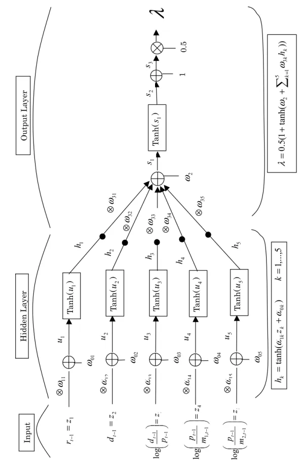
t’ which is described as follows.6The functional form used to generate the two forecasting parameters is assumed to be a feedforward neural network with a single hidden-unit with restricted inputs, which is
6 The linear forecasting model in (3) is optimal when agents believe that prices are a linear function of
dividends and a homogeneous rational expectation equilibrium obtains. But here there is no such
used in LeBaron (2002a) as follows.
)
tanh(
)
(
)
6
(
,
))
(
1
(
*
5
.
0
)
(
)
5
(
)
(
)
4
(
5 1 , 3 2 , 0 , , 1u
u
g
b
a
l
h
g
z
z
g
h
k k k t l k k t k k=
=
+
+
=
+
=
∑
=ω
ω
λ
ω
ω
.Neural network is a particular type of functional form often used in the field of biological nervous systems. Here since the information set, ‘
z
t’,consists of 5 variables, those are first combined with weights (ω
0kandω
1k for k=1,…,5) and transformed in a hidden layer, which is expressed as equation (4), and produce signals, h. Since the information set has 5 variables, hidden layers produce 5 signals in total (h
k for k=1,…,5). Those signals are connected with weights (ω
2andω
3k for k=1,…,5) and produce a signal,λ
, which is expressed as equation (5). ‘λ
’ lies between 0 and 1 by construction. We call “feedforward” since the direction of the signal is just one way from input, ‘z
t’, to output, ‘λ
’. Figure 3 is a picture for this neural network, equation (4) to (6).Permitting to range ‘
λ
’ with the allowable bounds for ‘ i ta
’ and ‘ i tb
’ in LeBaron(1999), that is,
a
∈
[
0
.
7
,
1
.
2
]
andb
∈
[
−
10
,
19
]
7, the forecast parameters ‘ i ta
’ and ‘ i tb
’are given by))
(
1
(
*
7
.
0
)
(
*
2
.
1
)
7
(
i a t a t tz
z
a
=
λ
+
−
λ
.))
(
1
(
*
)
10
(
)
(
*
19
)
8
(
i b t b t tz
z
b
=
λ
+
−
−
λ
.8Agents are heterogeneous in terms of their expectation since each has different values of weights in their own neural net.
Here agents build their forecast using the neural network. This is an extension from the financial market in LeBaron et al. (1999). The agents in LeBaron et al. (1999) forecast using what are called ‘condition-forecast’ rules.9
7 Those ranges are given to be centered around the rational expectation equilibrium values.
8 Each agent has two neural networks since he has two forecasting parameters. Since each has 16
parameters in his neural network, he has 32 in total.
3. Strategy making:
Based on the prediction, each agent i sets his demand for share as:
2 , 1 1
ˆ
)
1
(
)
(
ˆ
*
)
9
(
i d p t f t t i t iE
p
d
r
p
s
+ + ++
−
+
=
σ
γ
. 4. Price determination:The new equilibrium price,
p
t, is determined according to the market equilibrium condition as: N p r b d p a p s N i i t f i t t i N i t i t = + − + + =∑
∑
= =1 1 ˆ2 ) 1 ( ) ( ) ( ) 10 (σ
γ
where N is the number of agents in themarket (=30).
5. Volume determination and updating variance estimates: After revealing the price, forecasting parameters i
t
a
and i tb
are updated according to thefeedforward neural network, (4)-(6) to get i t
a
+1and i tb
+1, and trading volume is recorded. Theprice at time t is derived by solving equation (10). After the price is set, agents update their portfolio and trading volume is recorded.10 Once the equilibrium price
t
p
is revealed, agents change their forecasting rule, it
a
and i tb
. Then the market demand and supply become unbalanced. So,p
tclears the market only temporally. In this sensep
t is a temporary equilibrium price (LeBaron (2002b))11.Here supply and demand are somehow balancing in some unspecified market institution (Arthur et al (1996)). Agents calculate their desired holdings and submit their decisions to the market specialist who functions as a market maker. The specialist collects
defined endogenously. These states map into a forecast for the future price and dividend which is then converted to share demand through the agent’s demand function.”
10 Since there is one market maker and 30 traders, the trading volume is defined as
|
|
2
1
|
|
2
1
30 1 30 1+
∑
∑
=
i=y
i i=y
iv
, wherey
iis trader i’s trading volume.11 This model doesn’t say anything that wealthier people can affect the price. Usually trading by wealthier
bids and offers from agents, and announces a price that clears the market. So, this institution deals with buying and selling in real time. An investor, who wants to buy stock, can always buy stock while seller can always sell the stock in this market.
Wealth, w, for individual i is evolved according to:
)
)(
1
(
)
(
)
11
(
1 1 1 i t t i t f t t i t i ts
p
d
r
w
p
s
w
+=
++
++
+
−
.Each agent is initially allocated 20,000 units of cash.
6. Genetic Algorithm:
Steps 1-5 are repeated for S (=25) periods. Then genetic algorithm (GA)12 is invoked to update their forecasting parameters. The steps 1-5 with GA are repeated 500 times every 25 periods.
The GA manipulates the parameters, ‘
ω
’, in the neural network, equation (4)-(6), to improve the performance according to a fitness criterion. Here the fitness criterion is wealth-based utility of the past 25 periods which is given as:∑
=
= =125(
+1)
)
12
(
S t i t iU
w
V
)
exp(
)
(
w
t+1=
−
−
w
t+1U
where
γ
13γ
is a constant absolute risk aversion coefficient and assumed to be 0.5.The variance estimate is updated according to an exponentially weighted average of squared forecast error,
(
)
[
(
)
]
{
}
2 1 1 1 1 2 1 , , 2 , ,1
ˆ
)
1
1
(
ˆ
)
13
(
i t t t i t t t t i d p t i d p+=
−
τ
σ
+ −+
τ
p
+
d
−
a
−p
−+
d
−+
b
−σ
whereτ
is fixed at 75.All agents involve GA simultaneously. The more detailed steps of the GA are introduced next.
Steps of GA Implementation
12 For an introduction to GA, see Mitchell(1996), Haupt and Haupt (1998), Muhlenbein and
Schlierkamp-Voosen (1993), and Tokinaga (2000). Janikow and Michalewicz (1991) empirically compare floating point and binary based GAs using dynamic control problem. Wright (1991) applies genetic algorithms to optimization problems over several real parameters.
13 As simulation proceeds, the wealth is always normalized to be in 5-digit number dividing by 10 if one of
the wealth exceeds 100,000. When we evaluate the utility, the wealth is divided by 1,000,000 since the utility function is negative exponential.
GA implements to the parameters, ‘
ω
’, in the neural network, equation (4) to (6). This paper considers the markets with individual and social learning. So, GA is run at the individual and social levels. But the steps to implement GA are exactly the same for exactly the identical market structure for social and individual learning. So, the following explanation to implement GA can be applied to market structures both with social and individual learning.A GA consists of a set of operations which manipulate a given population. There is one population in a social learning economy which consists of 30 agents while an individual learning market has 30 populations each of which represents agent who has 30 ideas in her mind. In an individual (social) learning market, each idea (agent) has a set of 32 parameters in her neural network. In individual learning, “ideas” interact within each of the agent’s mind while “agents” interact in social learning. More specific explanations about GA are as follows.
1) Initialization of population:
The initial sets of parameters for each idea (agent) are chosen randomly from the range [-1,1]14. Since there are 30 ideas (agents), the matrix of parameters is 30x32.
2) Ranking and Selection:
In each generation n the agents face 25 (=S) portfolio decisions. The forecasting rules that did well according to the fitness measure will be more likely to be copied than a rule with a lower fitness. The forecasting rule for idea (agent) i is to be copied with the probability:
∑
=
∑
=
= = + = = 25 1 1 30 1)
(
/
1
/
1
)
14
(
S t i t i N j j i iw
U
V
where
V
V
P
.3) Crossover and Mutation:
The GA then introduces new rules through two genetic operators that manipulate some parameters of the population. These two operations are called crossover and mutation. The
algorithm chooses between crossover and mutation with equal probability. After either of crossover and mutation is selected, the algorithm randomly chooses one of the information variables. Then all of the parameters related to that information variable are subject to the crossover or mutation. For example, in Figure 3, when the algorithm chooses crossover (mutation) and information variable,
r
t−1, then the parameters,ω
11,
ω
01,
ω
31,
ω
2, in the selected pair of parents are subject to the crossover (mutation).15A selected set of the parameters in the neural network, which are related to one of the information variables, is crossed over. Intuitively, in social learning, for the crossover on forecasting parameters, two investors who have similar prediction skills are more likely to meet and exchange their opinions for the stock price prediction. They talk about a particular information variable for the prediction. After that, they update their prediction rule of that variable based on the discussion with other agents. For the crossover in individual learning, agents update their own ideas inside their mind.
Here the crossover for the real-valued GA is as follows. A new parameter (offspring) is produced by combining two parameters (parents) as:
(15) offspring=parent 1 +
α
* (parent 2 – parent 1).where
α
is a scaling factor chosen uniformly at random in the interval [-0.25,1.25]. A new ‘α
’ is generated for each pair of parents combined together (Muhlenbein and Schlierkamp-Voosen (1993)).For mutation on the real-valued GA, a parameter
ω
iis selected with probabilityp
m(=0.08) for mutation, and are added a small perturbation.16
15 A pair of parameters undergo crossover with a constant probability of 40% as in Lettau (1997).
16 A value out of an interval
[
,
]
i i
range
range
−
is added to the selected variable. The ‘range’ is defined as0.5 * [-1,1]. The new value
ω
i*
is computed according toδ
ω
ω
i*
=
i±
range
i .The + or – sign is chosen with probability 0.5.
δ
is computed from a distribution that prefers small values.This is realized as follows:
∑
− = −=
1 02
m i i iη
δ
. i4) Reinsertion:
After crossover or mutation is conducted, agents do “back-testing”. The fitness function (12) is calculated with updated parameters and observed prices. A set of the updated fitness is compared with the old fitness. The algorithm conducts insertion of the updated parameters into the current set of parameters when the new ones could produce higher fitness than the old ones do. Offsprings replace least fit parents.17
4. Experiments with Intelligent Agents
This section consists of two investigations in a market with evolution which allows agents to choose one rule at each period among a set of updated ideas produced through individual and social learning. First, the convergence property to the REE is examined with an intelligent economy, and it concludes that the intelligent economy cannot converge to the REE since intelligent agents are not rational. Second, it is examined which level of learning dominates the market. It shows that a wealthy agent picks an idea from individual learning more often than others do while poor agents imitate others.
More details of the evolution are as follows. When agents update their trading rules, they evaluate the past performance of a set of the ideas which are created in both individual and social learning, and choose one idea from them. Each agent has a set of 30 ideas which are updated in her mind. In addition, there are 30 agents in the market, each of whom has one idea for social learning. So, there are 30 ideas in total for social learning. After a GA is conducted, each agent is able to select one idea from 60 ideas by taking two steps. At the first stage, an agent picks two ideas, one of which is taken from individual learning and another from social learning. The ideas are evaluated according to the wealth-based fitness criterion (equation (12)). At the first stage, each agent is more likely to choose one idea which performed better in the past. In the second stage, she selects one from the selected two by comparing absolute values of the fitness.
The ideas used in individual and social learning are totally isolated in this setting. On the one hand, each agent has her private ideas, and never reveals them to others. These ideas are evolved only with individual learning. On the other hand, agents have some ideas, and are willing to reveal them, in order to get new information from other agents. So, in
this setting, each agent has two types of ideas, one of which is totally private while another is for social interaction.
Under this setting, the choice of the level of learning is not exogenous but endogenous. In addition, since each agent has a wider set of idea to choose in this economy, they are considered to be more “intelligent” than the agents in the previous sections. This section deals with such an economy with intelligent agents.
4.1 Are intelligent agents rational?
Simulations are repeated for 10 times under different random seeds to collect cross-sectional statistics. The series of stock price, dividend, and volumes are recorded for the last 5,000 periods, and the following statistics for returns and volumes are calculated, and compared with the economies which have only one level of learning, i.e., individual or social learning. In either individual or social learning economy, each agent can choose one rule from 30 rules while an economy with intelligent agents allows them to choose one from 60 rules created from both levels of learning. The statistics for returns series are the standard deviation, excess kurtosis, volatility clustering, and nonlinear dependence while for the volume series, the averages are calculated.
For the return series statistics, the following regression is first conducted with the simulated data:
(16)
p
t+1+
d
t+1=
α
+
β
(
p
t+
d
t)
+
ε
t.Following LeBaron et al. (1999), the estimated residual series
ε
ˆ
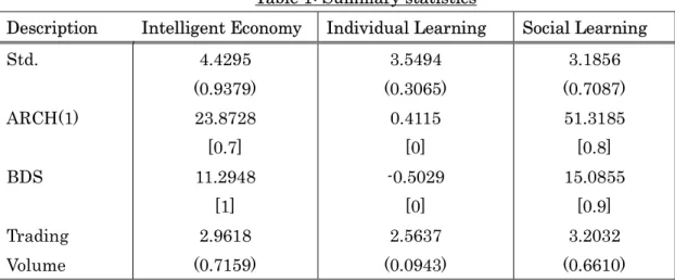
tare analyzed, and the results are in Table 1.Under the homogeneous rational expectation equilibrium, the residual time series follow independent and identical distribution with the standard deviation of 2 (N(0,4)). The standard deviations are 4.4295 in an economy with intelligent agents, 3.5494 in individual learning and 3.1856 in social learning. These show higher variability than should be in the homogeneous rational expectation equilibrium.
The ARCH test deals with the volatility clustering for the return series (Engle (1982)). It tests the null hypothesis that a time series of sample residuals is i.i.d. Gaussian disturbances (i.e., no ARCH effects exist). The numbers reported are the means of the test
statistics. The numbers in the brackets are the fraction of runs that rejected 'no ARCH' at the 95% confidence level.18 When an economy with intelligent agents is in the rational expectation equilibrium, there should be no ARCH phenomena. But the no ARCH null hypothesis is rejected 8 times in an intelligent agent economy. The result indicates the ARCH dependence in the residuals in the economy.
Table 1: Summary statistics
Description Intelligent Economy Individual Learning Social Learning Std. ARCH(1) BDS Trading Volume 4.4295 (0.9379) 23.8728 [0.7] 11.2948 [1] 2.9618 (0.7159) 3.5494 (0.3065) 0.4115 [0] -0.5029 [0] 2.5637 (0.0943) 3.1856 (0.7087) 51.3185 [0.8] 15.0855 [0.9] 3.2032 (0.6610)
Note for Table 1: Means over 10 runs. Numbers in parenthesis are standard errors estimated using the 10 runs. Numbers in brackets are the fraction of tests rejecting the no ARCH, or independent identically distributed null hypothesis for the ARCH and BDS tests, respectively, at the 95% confidence level.
Nonlinear dependence asks if the return series are identically and independently distributed over time. It is tested with the BDS (Brock, Dechert, and Scheinkman) statistic (Brock, Dechert, Scheinkman, and LeBaron (1996)). The BDS test is conducted with the null hypothesis that a time series sample comes from an IID data generating process.19 Under the homogeneous rational expectation equilibrium, the null on BDS test cannot be rejected. However, the IID null hypothesis is rejected 9 times in an economy with intelligent agents. The result shows that there are some correlated patterns on data generating process in the economy with intelligent agents.
18 The test procedure is to run the OLS regression and save the residuals. Then we regress the squared
residuals on a constant and p lags. The asymptotic test statistic is
M
*
R
2, where M is the number ofsquared residuals included in the regression and
R
2 is the sample multiple correlation coefficient. It isasymptotically Chi-Square distributed with p degrees of freedom under the null hypothesis.
19 The alternative hypothesis is not specified. But this test has good power against nonlinear alternatives.
The fifth row is the results for the trading volume. In standard efficient market financial theory, identical investors share rational expectations of an asset’s future price. Taking into account all market information, the investors make an investment decision which clears the market. So, in the standard financial theory, there is no opportunities left open for speculative profit except by luck. In this case, the trading volume is low or zero20. The results show that the average trading volumes over the final 5000 periods are not zero in all economies.
The results are totally opposite to what the homogeneous rational expectation equilibrium says. The economy with more intelligent agents cannot reach the REE as in an economy with either individual or social learning. Agents don’t behave rationally when they are intelligent. Intelligent agents are not rational.
Why doesn’t the market with intelligent agents converge to the REE? Each agent has 60 ideas, each 30 of which are from individual and social learning. Agents update their ideas every 25 periods, and choose one which could achieve higher wealth-based fitness. When the stock price moves much higher level than that of the REE during the 25 periods, agents take the information of the higher level of the prices into account to update their ideas. Agents choose ideas to get higher level of wealth, but those ideas reflect such higher price levels in those periods. During the period of higher variation of the stock price than the REE series, the ideas would reflect such higher variations. So, as far as the price series behave differently from the REE, the ideas are also far from the REE. As a result, the economy never converges to the REE. It would be the only way to reach the REE that agents adapt their forecasts very slowly to new observations as in LeBaron (2000) and Arthur et al. (1996).
In the real world, investors in the stock market have become more intelligent than those in, for example, 40 years ago. They have now more sophisticated ways in analyzing the stock market and forecasting future prices, and so on. However, does that mean that the recent stock market behaves rationally? Definitely, it doesn’t. The stock market behaves in opposite ways to what the rational expectation theory says. The market with intelligent investors is not related to the rationality at all.
4.2 Which Level of Learning Dominates the Market?
20 For liquidity purpose, agents may liquidate (trade) some amount of their own assets. In this case,
Agents in the second experiment can choose ideas from both levels of learning. They basically choose an idea which performed well in the past. Since the fitness function is the wealth-based utility, it is considered as a better idea that could produce higher wealth over a particular past time span. This section investigates a hypothesis that agents who accumulate more wealth in the past are more likely to pick an idea from individual learning than others do while some who have less wealth are more likely to adopt an idea from social learning. Most of the agents follow the herd, and only agents with very high wealth would rely on private ideas. The matrix on the choice of learning levels and the matrix on wealth in the last 5000 periods of 10 simulations are used for the investigation, both of which are described as follows.
Data:
At each generation in a simulation with 500 generations, the choices of the level of learning by agents are stored with 0 if she chose individual learning and 1 if it is social learning. There are 200 generations in the last 5000 periods. Since we have 30 agents in a market, the matrix on the choices is eventually 30x200. For the matrix on wealth, the wealth of each agent over a generation is summed up (the sum of the 25 periods’ wealth). Since we have 200 generations in the last 5000 periods, the dimension of the matrix on wealth is 30x200. At each generation, taking the matrix on the choices as a dependent variable and the matrix on wealth as an independent variable, the parameters in the following model (equation (17)) is estimated.
Model:
Since the dependent variable consists of only 0 and 1, it is convenient to use the binary choice model which links the decision by agents to the wealth variable. The hypothesis is that less wealthy agents are more likely to choose social learning. Using the logistic function, the following probability to choose social learning is useful to analyze the hypothesis.
(17) P(y=1|wealth) =
WEALTH WEALTHe
e
1 0 1 01
β β β β + ++
.A variable, WEALTH, needs to be standardized to have small numbers for this type of probability function.21 The parameters,
0
β
andβ
1, of this logit model are estimated by the maximum likelihood method.Analyses:
There are 200 sets of choice and wealth variables for 30 agents. The parameters are estimated generation by generation to get 200 sets of
β
0 andβ
1. With the parameter estimates, the estimated probabilities are calculated for each agent and for all generations. Our hypothesis which poorer agents are more likely to choose ideas from social learning suggests that there is a negative relation between the probability to choose social learning and the wealth level. So, the estimated probabilities and the wealth levels are compared for all 30 agents and for all 200 generations.As a first investigation, at each generation agents are categorized into the ones who have wealth “more than average” at the generation and the ones who have wealth “less than average”. The estimated probabilities are categorized into “more than 0.5” and “less than 0.5”. If the probabilities are “more than 0.5”, that agent is more likely to pick an idea from social learning. The following four cases are investigated.
(Case 1): Agents with ”more than average wealth” are more likely to choose ideas from
individual learning while agents with “less than average wealth” are more likely to choose ideas from individual learning also.
(Case 2): Agents with “more than average wealth” are more likely to choose ideas from
individual learning while agents with “less than average wealth” are more likely to choose ideas from social learning.
(Case 3): Agents with “more than average wealth” are more likely to choose ideas from
social learning while agents with “less than average wealth” are more likely to choose ideas from individual learning.
(Case 4): Agents with “more than average wealth” are more likely to choose ideas from
social learning while agents with “less than average wealth” are more likely to choose ideas
from social learning also.
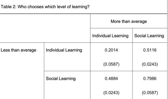
The numbers in Table 2 shows the fractions of agents in whole periods corresponding in each case.22 The numbers in parenthesis are the standard deviations across 10 simulations.
The number in the upper-left corner is the fraction representing two types of agents. Those are the agents, who have more than average wealth and involve individual learning, and the ones, who have less than average wealth and associated with individual learning. Around 20% of all agents in whole periods correspond to this case. The number in down-left corner is the fraction associated with “Case 2” which is about 49% while that in upper-right corner represents “Case 3” which is about 51%. The number is down-right corner shows the highest. This is the fraction satisfying the following two types of agents. Those are the agents who have more than average wealth and involve social learning, and
those who have less than average wealth with social learning. The result shows that about 80% of the agents are more likely to choose ideas from social learning over the whole periods.
The analysis so far categorized the wealth levels into only two, i.e., “more than average” and “less than average”. So the behavior of the agents who have really high
22 Each of the fraction is the average across 10 simulations.
Table 2: Who chooses which level of learning?
More than average
Individual Learning Social Learning
Less than average Individual Learning 0.2014 0.5116
(0.0587) (0.0243)
Social Learning 0.4884 0.7986
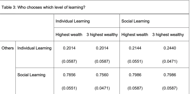
wealth is not clear from the analysis. The following examines the behavior of agents who have highest wealth and are the three highest wealthy at each generation. Two of the important results in Table 3 are as follows.
(Result 1): Agents with “high wealth” in each generation are more likely to choose ideas from individual learning while other agents are more likely to choose ideas from social learning.
(Result 2): Agents who have “high wealth” in each generation are more likely to choose ideas from social learning while other agents are more likely to choose ideas from social learning also.
For example, about 79% of agents are the ones, some of whom with the highest wealth at a particular generation choose ideas from individual learning (or social learning), and some of the others involve social learning. For the wealthy agent, the numbers are quite high regardless of the levels of learning. But the ideas in individual learning is more frequently selected by the wealthy than the others do. So, we would conclude that when agents have really high wealth, they are more likely to choose their own ideas than other agents do. The other agents are more likely to involve social learning.
Table 3: Who chooses which level of learning?
Individual Learning Social Learning
Highest wealth 3 highest wealthy Highest wealth 3 highest wealthy
Others Individual Learning 0.2014 0.2014 0.2144 0.2440
(0.0587) (0.0587) (0.0551) (0.0471)
Social Learning 0.7856 0.7560 0.7986 0.7986
These two results are the same for the cases of the three highest wealthy agents. But the fraction for the wealthy agents using individual learning is decreasing as taking more wealthy agents into account, given that the others choose social learning. Agents use their private ideas more often than the others do only when they have really high wealth. In other words, most of the agents follow social learning since the social learning would possibly produce better ideas. The social learning dominates the market.
The results indicate that the wealth level of each agent is important for choosing a level of learning. It would be because the fitness function in this paper is wealth-based utility. However, if the fitness function is based on, for example, “prediction accuracy”, we would reach a conclusion that an agent with more accurate forecasting methods is more likely to choose individual learning than others do. Regardless of the fitness function we specify, it would be concluded that the social learning dominates the market, and most agents would be better off by constraining the use of their own ideas.
5. Conclusion
This paper introduces a learning and adaptation mechanism which allows agents to choose one rule among a set of ideas updated through both individual and social learning, and mainly showed the following two results. First, the time series from an economy with intelligent agents doesn’t show a convergence to a homogeneous rational expectation equilibrium. The second investigates which level of learning is likely to dominate in the market. It concludes that the social learning dominates the market. Agents would be better off in an ex ante welfare sense by constraining the use of their own ideas.
References
Arifovic, Jasmina. “The Behavior of the Exchange Rate in the Genetic Algorithm and
Experimental Economies.” Journal of Political Economy vol.104 no.3 (1996): 510-541.
Arifovic, Jasmina, and Gencay, Ramazan. “Statistical Properties of Genetic Learning in a Model
of Exchange rate.” Journal of Economic Dynamics and Control 24 (2000): 981-1005.
Arifovic, Jasmina. “Evolutionary Dynamics of Currency Substitution.” Journal of Economic
Dynamics and Control 25 (2001a): 395-417.
Persistent Exchange-Rate Volatility.” Macroeconomic Dynamics 5 (2001b): 204-224.
Arifovic, Jasmina. “Exchange Rate Volatility in the Artificial Foreign Exchange Market.” In:
Chen, Shu-Heng (eds.), Evolutionary Computation in Economics and Finance. Physica-Verlag, (2002):
123-134.
Arthur, W.B., Holland, J., LeBaron, B., Palmer, R., and Tayler, P. “Asset Pricing under Endogenous Expectations in an Artificial Stock Market.” In W. B. Arthur, S. Durlauf, and D. Lane, eds,
The Economy as an Evolving Complex System II, Addison-Wesley, Reading, MA, (1996): 15-44.
Bikhchandani, Sushil, Hirshleifer, David, and Welch, Ivo. “Learning from the Behavior of
Others: Conformity, Fads, and Informational Cascades.” The Journal of Economic Perspectives 12 (1998):
151-170.
Brock, W. A., Dechert, W. D., Scheinkman, J. A., and LeBaron, B. “A Test for Independence Based
on the Correlation Dimension.” Econometric reviews. 15 (3) (1996): 197-235.
Chen, Shu-Heng, and Yeh, Chia-Hsuan. “Evolving Traders and the Business School with Genetic
Programming: A New Architecture of the Agent-Based Artificial Stock Market.” Journal of Economic
Dynamics and Control 25 (2001): 363-393.
Devenow, Andrea, and Welch, Ivo. “Rational Herding in Financial Markets.” European Economic
Review 40 (1996): 603-616.
Engle, Robert F. “Autoregressive Conditional Heteroscedasticity with Estimates of the Variance
of United Kingdom Inflation.” Econometrica 50 (1982): 987-1008.
Goodhart, Charles A. E., and O’Hara, Maureen. “High Frequency Data in Financial Markets:
Issues and Applications.” Journal of Empirical Finance 4 (1997): 73-114.
Graham, John R. “Herding among Investment Newsletters: Theory and Evidence.” The Journal
of Finance 54 (1999): 237-268.
Haupt, Randy L., and Haupt, Sue Ellen. “Practical Genetic Algorithms.” John Wiley and Sons, (1998).
Janikow, Cezary Z., and Michalewicz, Zbigniew. “An Experimental Comparison of Binary and Floating Point Representations in Genetic Algorithms.” In: Belew, Richard K., and Booker Lashon B. (eds.),
Proceedings of the Fourth International Conference on Genetic Algorithms Morgan Kaufmann, (1991): 31-36.
LeBaron, Blake, Arthur, W. Brian, and Palmer, Richard. “Time Series Properties of An Artificial
Stock Market.” Journal of Economic Dynamics and Control 23 (1999): 1487-1516.
LeBaron, Blake. “Evolution and Time Horizons in an Agent-Based Stock Market.”
LeBaron, B. “Calibrating an Agent-Based Financial Market.” Technical report, Brandeis University, Waltham, MA, (2002a).
LeBaron, Blake. “Building the Santa Fe Artificial Stock Market.” Technical Report, Brandeis University (2002b).
Lettau, Martin. “Explaining the Facts with Adaptive Agents: The Case of Mutual Fund Flows.”
Journal of Economic Dynamics and Control 21 (1997): 1117-1147.
Mitchell, Melanie. “An Introduction to Genetic Algorithms.” MIT press, (1996).
Tay, Nicholas S. P., and Linn, Scott C. “Fuzzy Inductive Reasoning, Expectation Formation and
the Behavior of Security Prices.” Journal of Economic Dynamics and Control 25 (2001): 321-361.
Tokinaga, Syozo. “Analysis of Economic Model through Complex System.” Kyusyu University Press, (2000), (Japanese).
Vriend, Nicolaas J. “An Illustration of the Essential Difference between Individual and Social
Learning, and its Consequences for Computational Analyses.” Journal of Economic Dynamics and Control
24 (2000): 1-19.
Wright, Alden H. “Genetic Algorithms for Real Parameter Optimization.” In: Rawlins, Gregory J.
E. (eds.), Foundations of Genetic Algorithms Morgan Kaufmann, (1991): 205-218.
Yeh, Chia-Hsuan, and Chen, Shu-Heng. “Toward an Integration of Social Learning Nd Individual Learning in Agent-Based Computational Stock Markets: The Approach Based on Population
Genetic Programming.” Computing in Economics and Finance (2000): Society for Computational
25 Fi gu re 3: A Fe ed fo rw ar d N eu ral N et w or k w it h a S in gl e H idde n -U n it w it h 5 i n pu ts ( E qu at io n (4) , ( 5) , an d ( 6) Inp u t 1 1