Statistical Downscaling and Bias Correction of Climate Model Outputs for Climate Change Impact Assessment in the U.S. Northeast

Statistical downscaling and bias correction of climate model outputs for climate

change impact assessment in the U.S. northeast

Kazi Farzan Ahmed

, Guiling Wang

⁎, John Silander

, Adam M. Wilson

, Jenica M. Allen

,

Radley Horton

, Richard Anyah

a_{Department of Civil and Environmental Engineering, University of Connecticut, United States}

b

Department of Ecology and Evolutionary Biology, University of Connecticut, United States c

Center for Climate Systems Research, Columbia University and NASA Goddard Institute for Space Studies, United States d

Department of Natural Resources and the Environment, University of Connecticut, United States

a b s t r a c t

a r t i c l e i n f o

Article history: Received 9 March 2012 Accepted 11 November 2012 Available online 20 November 2012 Keywords:

bias correction

climate change impact analysis extreme climate index statistical downscaling

Statistical downscaling can be used to efficiently downscale a large number of General Circulation Model (GCM) outputs to afine temporal and spatial scale. To facilitate regional impact assessments, this study statistically downscales (to 1∕8° spatial resolution) and corrects the bias of daily maximum and minimum temperature and daily precipitation data from six GCMs and four Regional Climate Models (RCMs) for the northeast United States (US) using the Statistical Downscaling and Bias Correction (SDBC) approach. Based on these downscaled data from multiple models,five extreme indices were analyzed for the future climate to quantify future changes of climate extremes. For a subset of models and indices, results based on raw and bias corrected model outputs for the present-day climate were compared with observations, which dem-onstrated that bias correction is important not only for GCM outputs, but also for RCM outputs. For future cli-mate, bias correction led to a higher level of agreements among the models in predicting the magnitude and capturing the spatial pattern of the extreme climate indices. We found that the incorporation of dynamical downscaling as an intermediate step does not lead to considerable differences in the results of statistical downscaling for the study domain.

© 2012 Elsevier B.V. All rights reserved.

1. Introduction

The term“climate change”refers to a persistent, and sometimes irreversible, shift in the long-term statistics of climate variables in a specific region or the entire globe. Increase in the atmospheric con-centrations of greenhouse gases appears to be the predominant cause of recent climate change. The Fourth Assessment Report (AR4) of the Intergovernmental Panel on Climate Change (IPCC) esti-mated that the global atmospheric concentration of CO2 increased from a pre-industrial value of about 280 ppm to 379 ppm in 2005, and the most conservative projection (following the emission scenar-io SRES B1) of atmospheric CO2concentration by the year of 2100 is at about 600 ppm. The CO2-induced climate change, which has already started to impact different sectors around the globe, is expected to become more evident in future decades with far-reaching impact in many sectors. Therefore, assessments of climate change impact, both global and regional, are drawing attentions from different groups of researchers and stakeholders.

All impact assessments require climate data at various spatial and temporal scales. Observed daily climate data, usually at sufficiently fine resolution, are available to perform such impact studies for past decades. However, the lack of daily temperature and precipitation data for future climate at adequately high spatial resolution has been a major obstacle to performingfine-scale analyses of future cli-mate change. Although General Circulation Models (GCMs) are the typical sources for future climate predictions, the spatial resolutions of those model outputs are too coarse to be directly used infine-scale impact studies. Moreover, all model outputs involve a great deal of biases that, if not corrected, can lead to significant errors in impact assessments. Therefore, spatial downscaling and bias correction of GCM outputs are necessary before their use in regional impact analysis (Giorgi and Mearns, 1991; Kidson and Thompson, 1998; Murphy, 1999). There are two distinct approaches to downscaling GCM outputs—

dynamic downscaling using a Regional Climate Model (RCM) and statistical downscaling. Dynamic downscaling is computationally ex-pensive. It is therefore not always feasible to perform dynamic down-scaling at the required spatial resolution, especially if predictions from multiple models are desired. For North America, dynamically downscaled climate data at daily resolution are available from the North American Regional Climate Change Assessment Program (NARCCAP). However, the spatial resolution of the NARCCAP data

Global and Planetary Change 100 (2013) 320–332

⁎ Corresponding author at: Department of Civil and Environmental Engineering, University of Connecticut, Storrs, CT 06269-2037, United States. Tel.: +1 860 486 3548; fax: +1 860 486 2298.

E-mail address:[email protected](G. Wang).

0921-8181/$–see front matter © 2012 Elsevier B.V. All rights reserved. http://dx.doi.org/10.1016/j.gloplacha.2012.11.003

Contents lists available atSciVerse ScienceDirect

Global and Planetary Change

(0.5° × 0.5°) is still not high enough for most impact assessments at local and regional scales. In addition, the outputs from RCMs, too, are likely to contain biases that need to be removed (Marinucci and Giorgi, 1992; Chen et al., 1999). In contrast, statistical downscaling is computationally efficient and can be suitably used to perform the spatial downscaling and bias correction for a large amount of GCM outputs, and has become a commonly used tool in impact studies. Various studies demonstrated that the overall performance of statistical and dynamic downscaling were similar in reproducing the present-day climate for the respective regions (Murphy, 1999; Wilby et al., 2000). In an extensive study, comparing the capacity of statistically and dynamically downscaled data to reproduce the observed re-gional hydrology,Wood et al. (2004)showed that dynamical down-scaling did not provide any additional skill in the context of their study.

Most statistical downscaling approaches are developed based on the assumption that the statistical relationship between large-scale GCM outputs and fine-scale observational data established for the present-day climate will remain unchanged in future climate (Wilby et al., 1998; Boé et al., 2006). For precipitation, conventional statistical downscaling methods use the empirical relationship between large-scale circulation-based predictor variables (geopotential heights, spe-cific humidity, cloud cover, etc.) and regional climate variables (precip-itation) that need to be estimated (Zorita and von Storch, 1999; Wilby and Wigley, 2000; Feddersen and Andersen, 2004). Recently, some sim-pler downscaling methods have been developed that directly use GCM precipitation as a predictor and involve bias correction of model outputs (Widmann et al., 2003; Wood et al., 2004; Schmidli et al., 2006; Iizumi et al., 2011). The performance of bias corrected and statistically downscaled climate model outputs was satisfactory in different hydroclimatological studies (Wilby et al., 2000; Wood et al., 2002; Dettinger et al., 2004). The Bias Correction and Spatial Disaggregation (BCSD) method, a probability mapping approach to correcting bias and downscaling climate model outputs as described inWood et al. (2002)or its variations, was adopted by several studies to assess the hy-drological impacts of climate change (Payne et al., 2004; VanRheenen et al., 2004; Hayhoe et al., 2006).Wood et al. (2004)investigated the per-formances of three different approaches of statistical downscaling methods for GCM outputs and the effects of incorporating RCMs as an intermediate process in hydrologic simulations. They showed that when applied to both raw GCM data and dynamically downscaled GCM data, the method developed byWood et al. (2002)produces sim-ilar results in retrospective hydrologic simulations.

The Bias Correction and Constructed Analogs (BCCA) method, de-veloped byMaurer and Hidalgo (2008), performs a“lumped”bias correction based on the month-speci_fic probability distribution of daily data followed by the constructed analogs approach to statistical-ly downscale climate models' daistatistical-ly output. Different than the BCSD approach that corrects the bias at each grid cell independently, the BCCA method is based on the linear regression of a collection of his-torically observed weather patterns that closely resemble the GCM weather pattern for each specific day, and therefore, is more dynamics-based.Maurer et al. (2010)demonstrated that statistically downscaled NCEP/NCAR reanalysis data using the BCCA method suc-cessfully reproduced daily stream flow observed at 11 stations in California.Abatzoglou and Brown (2011, henceforth AB11)showed that a modified BCSD method, where a 15-day moving window is used to define the probability distribution of daily data for bias cor-rection following the spatial interpolation of GCM outputs to the downscaled grid, performed reasonably well in producingfine-scale daily meteorological data required for wildfire analysis.

In this study, using a modification of the BCSD approach, which is referred to as the Statistical Downscaling and Bias Correction (SDBC) method hereafter, we create a dataset of daily maximum and mini-mum temperature and daily precipitation for direct use in ecological or other impact assessments of climate change for the New England

region, at a spatial resolution of 1∕8° × 1∕8° for the future period of 2046_–2065. Based on these data, we aim to evaluate the importance of bias correction of model outputs before their use in regional impact studies and analyze the effectiveness of the SDBC method in address-ing the model-related uncertainties in future climate predictions. Using a few temperature and precipitation extreme indicators as examples, we also assess the effect of conducting dynamical down-scaling as an intermediate step before statistical downdown-scaling, by comparing the SDBC results from RCMs and those from their driving GCMs.

Section 2describes the data, methodology and de_finitions of the extreme indicators.Section 3presents results on the impact of bias correction on reducing model-related uncertainties taking one ex-treme precipitation indicator for example, and discusses the future pattern offive extreme indicators estimated based on the statistically downscaled and bias corrected model outputs.Section 4summarizes the results and presents the conclusion.

2. Data and methods

2.1. Spatial downscaling and bias correction

Daily precipitation, maximum temperature and minimum tem-perature data during the future period of 2046_–2065 from six GCMs and four RCMs are statistically downscaled to the spatial resolution of 1∕8° × 1∕8° in this study. The study area, that includes the New England region, ranges from 67.0625 W to 75.0625 W in longitudes and from 38.8125 N to 48.8125 N in latitudes. The GCM simulations are taken from the World Climate Research Program (WCRP)'s phase 3 of the Coupled Model Intercomparison Project (CMIP3), and include those from CCSM, GFDL, PCM, CGCM, MPI and MIROC. These GCMs are so chosen that they cover the full range of model sensitivity to changes in the atmospheric CO2concentration as found in IPCC AR4. The RCM simulations are taken from the NARCCAP database that provides high resolution climate simulation using different RCMs driven by outputs from a number of GCMs. For the analysis of temperature extremes, the RCM–GCM combinations are RCM–CGCM, CRCM–CGCM, CRCM–

CCSM and WRFG–CCSM. In the case of precipitation extremes, RCM–

GFDL replaced CRCM–CCSM. These combinations were chosen based on data availability at the beginning of this study. Since NARCCAP data is available for emission scenario SRES A2 only, GCM output is also taken from the SRES A2 scenario for consistency.

The SDBC method proposed in this study is a modification of the BCSD approach ofWood et al. (2002, 2004)andMaurer (2007). One limitation of the BCSD method, like most statistical downscaling ap-proaches, is the sensitivity of thefinally downscaled results to the ini-tial spaini-tial resolution at which bias correction is applied. For example, in the case of precipitation, the coarser initial resolution may lead to an underestimation of frequency and magnitude of the extreme events. In order to address this uncertainty, in the SDBC method, raw GCM and RCM outputs are statistically downscaled to thefinal

Table 1

Extreme climate indicators which were selected and analyzed in this study. Extreme

Indicators

Definitions Unit

Fd Total number of frost days, defined as the number of days per year with minimum temperature below 0 °C

Days GSL Growing season length, defined as the period between the

first spell offive consecutive days with mean temperature above 5 °C and thefirst spell offive consecutive days with mean temperature below 5 °C

Days

TGO Time when the greenup onset occurs in the spring Julian day

R5d Maximum 5-day total precipitation mm

Fig. 1. Future mean (2046 – 2065) of total number of days with precipitation greater than 10 mm from raw GFDL and spatially downscaled and bias corrected GFDL data using the BCSD, the BCCA, the Abatzoglou and Brown, and the SDBC methods (top row), and respective predicted changes from present-day mean (1961 – 1999) (bottom row).

spatial resolution prior to correcting the bias. A similar modification was made by AB11, where the raw model outputs were spatially in-terpolated before bias correction was performed.Li et al. (2010), in their study on bias correction of monthly precipitation and tempera-ture, also regridded coarse-scale model data to the same resolution as the observation before correcting the bias in order to address the un-certainties related to interpolation along with model bias. In this study, the downscaling is applied to a“factor value”. The“factor”for precipitation is the ratio of model precipitation to observed precipita-tion aggregated to the model resoluprecipita-tion, and for temperature is the difference between model temperature and observed temperature ag-gregated to the model resolution. The downscaling of the factor values follows the synergraphic mapping system (SYMAP) algorithm devel-oped byShepard (1968). Combining the downscaled factor with the fine resolution observational data (multiplication for precipitation and addition for temperature) produces a downscaled model output, which retains the model climatology but derives its fine-resolution spatial pattern from observations. Bias correction (following the probability mapping approach) is then applied as a last step to correct the remaining model bias.

The bias correction algorithm of the BCSD method is based on the comparison between the Cumulative Distribution Function (CDF) for the observed climate and that for a given GCM (or RCM) outputs dur-ing the same time period. It assumes that the model biases in both present and future climate simulations follow the same pattern. The observed temperature and precipitation data used in this study are taken from the dataset developed by Maurer et al. (2002). This dataset, having a spatial resolution of 1∕8° × 1∕8° and spanning the period of 1951–2010, was derived from the National Oceanic and

Atmospheric Administration (NOAA) Cooperative Observer (Co-op) stations data. The Co-op data were gridded to the 1∕8° resolution using the SYMAP algorithm. However, in order to perform the bias correction for daily data, both the BCCA and the AB11 method adopted the lumped approach to define the quantile map instead of restricting the distribution to a specific Julian day of interest. Similarly, in this study, the CDF is calculated based on the month-specific probability distribution of daily data of the present-day climate.

In models, it rains almost every day at lower rain intensity, while in observation there are many zero precipitation days and the rain in-tensity during the rainy days is larger than in models. That creates an inconsistency between the daily precipitation CDF of the model and that of the observational data. In order to address this problem, we modified the CDF of model precipitation data. Specifically, if P0is the probability threshold of having zero precipitation days in the ob-served climatology, the values of any model precipitation having probability threshold lower than P0were set to zero. As such, the CDFs of both model and observed data were made consistent. One drawback, however, is that many drizzling days are set to no-rain days, which leads to slight underestimation of the rain amount.

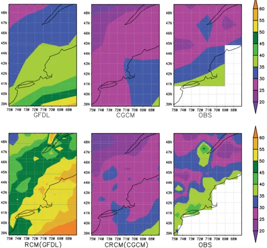
Fig. 2.Mean values of total number of days with precipitation greater than 10 mm in present climate which were calculated using raw GCM simulations (1961–1999) at 2° and

dynamically downscaled RCM simulations (1971–1995) at 0.5° and their comparisons with observation at their corresponding resolutions.

Table 2

Root-mean-square error (RMSE) and coefficient of determination (R2

) for present-day (1971–1995) mean of R10, based on comparison of model present-day climate against observation.

Model GFDL CGCM RCM_GFDL CRCM_CGCM

RMSE 4.94 5.14 13.13 26.22

R2

2.2. Climate extremes

Table 1 lists the definitions for the extreme climate indicators discussed in this study—three indicators for extreme temperature and two indicators for extreme precipitation. Four out of thesefive indi-cators, apart from the Time for Greenup Onset (TGO), follow the defi ni-tions inFrich et al. (2002)and such definitions have been used in other studies (Tebaldi et al., 2006; Orlowsky and Seneviratne, 2011). Despite potential limitations related to the use of afixed threshold (Kiktev et al., 2003; Alexander et al., 2006), thesefive indicators are chosen here for their strong relevance to plant ecology (an area this study was originally designed to serve). TGO was added in this study in order to see how changes in the maximum and minimum temperature may alter vegeta-tion phenology. The greenup onset was determined by calculating the Growing Degree Days (GDD) for plants. In this study, the day of the year when the value of GDD reaches 150 was considered as the be-ginning of greenup according to the Integrated Biosphere Simulator (IBIS) vegetation model (Foley et al., 1996; Kucharik et al., 2000).

Tebaldi et al. (2006)analyzed the historical and future changes in extreme events based on ten extreme indicators (defined byFrich et al., 2002) using the multi-model ensembles of nine GCMs participat-ing in IPCC-AR4. A follow-up study byOrlowsky and Seneviratne (2011)expanded the Tebaldi et al. (2006)study for the complete dataset of available GCMs for the emission scenario SRES A2 including the analysis at seasonal time scales. While these studies were instru-mental in setting the stage for further studies on climate extremes in future years, they lack direct applicability for regional studies because of the coarse spatial resolution of GCM outputs and the biases associ-ated with them. In this study, spatial downscaling and bias correction

are conducted to make the results more accurate for the small region of interest.

2.3. Comparison with other similar approaches

Here we compare the performance of four different statistical downscaling methods for daily climate data in predicting the future changes in climate extremes, using R10 and the GFDL model as an ex-ample. Future mean (2046_–2065) for R10, which were calculated from the bias corrected and downscaled GFDL outputs following the original BCSD, the BCCA, the AB11, and the SDBC method, and the predicted change from present-day climate (1961_–1999) are com-pared (Fig. 1). For the original BCSD data, we performed the bias cor-rection and downscaling following the methodology ofWood et al. (2002)where the quantile maps for daily data were defined based on the probability distribution of a specific Julian day of interest. After the bias correction, the“factor” values (as defined inSection 2.1) were

Fig. 3.Future mean (2046–2065) of total number of days with precipitation greater than 10 mm for GCMs (2°) and RCMs (0.5°), based on raw (top row) and bias corrected (bottom

row) outputs.

Table 3

Root-mean-square deviation (RMSD) and coefficient of determination (R2_{) between} two models for future (2046–2065) mean of R10, based on raw model output and bias corrected model outputs.

Models GFDL and CGCM RCM_GFDL and CRCM_CGCM

(Raw/bias corrected) (Raw/bias corrected)

RMSD 8.81/2.58 22.35/2.09

R2

calculated and downscaled to produce climate data at thefinal resolu-tion. For the AB11 data, following the methodology ofAbatzoglou and Brown (2011), wefirst spatially interpolated the coarse-scale model output to thefinal resolution prior to performing the bias correction where quantile maps were defined using the lumped approach. The BCCA data was downloaded from the“Bias Corrected and Downscaled WCRP CMIP3 Climate Projections”archive athttp://gdo-dcp.ucllnl.org/ downscaled_cmip3_projections. Future changes of R10 derived from the raw GFDL output feature an overall increase for the northeast US. However, the original BCSD approach predicts a decrease over a large region, while results from the BCCA method show a decrease in R10 for the entire region. Both the AB11 and the SDBC, with very similar re-sults for future mean of R10, perform better in retaining the signal from the raw GCM to predict the future changes of extreme precipitation.

3. Results and discussions

A major challenge in using model outputs in impact assessments is the strong model-dependency of future predictions due to unavoidable model biases. The use of bias correction in this study reduces the range of such model uncertainties. As an example, the climatic mean of R10, calculated using the outputs from GFDL and CGCM interpolated at 2° spatial resolution, were compared with the observed mean for the peri-od of 1961–1999 (calculated using theMaurer et al. (2002)dataset spatially aggregated from 1∕8° to 2°) (top row ofFig. 2). GFDL overesti-mates the mean value for R10, while CGCM tends to underestimate. Similar analysis of R10 for the period of 1971–1995 was performed using dynamically downscaled GCM outputs from two NARCCAP

combinations, RCM-GFDL and CRCM-CGCM, at a spatial resolution of 0.5° (bottom row ofFig. 2). The difference between the model outputs and observed data appears to increase after the dynamic downscaling of GFDL output using RegCM, and the level of underestimation in CRCM_CGCM is similar to that in CGCM. The values of root-mean-square error (RMSE, the root-mean-square root of the mean root-mean-squared deviation) and coefficient of determination (R2_{) between model prediction and} observations for present-day (1971–1995) mean of R10 show that after the dynamic downscaling of GCM data, model biases still remain or even become larger (Table 2). Various studies showed that biases in the driving GCM can be ampli_fied by RCM because of the systematic errors in boundary forcing in unconstrained dynamic downscaling (Christensen et al., 1998; Noguer et al., 1998). It is worth mentioning that although disagreements exist among different models, all of them capture the main spatial patterns for the mean value of R10, with a gradual increase of heavy precipitation event from inland to the coast. However, the comparison between the model simulation and observed data, when they were used to perform extreme climate analysis, makes it evident that both GCM and RCM simulations can involve a great deal of biases.

The mean values of R10 for the future period of 2046–2065 calcu-lated using daily precipitation data from GCM and RCM simulations before and after bias correction show variable levels of model dis-agreement depending on bias correction (Fig. 3). Without bias correc-tion, model predictions involve a large degree of uncertainties. For the raw GCM data (top row), the mean value of future R10 in the GFDL model is higher than that in the CGCM for most of the region. Similar comparison between RCM–GFDL and CRCM–CGCM simulations

shows a larger disagreement, with RCM–GFDL always predicting a greater number of heavy precipitation events. The model-related vari-ability decreases when the model outputs are used to perform similar analysis after they are bias corrected (but not downscaled) following the bias correction algorithm of the SDBC method (bottom row). The similarity in the spatial patterns captured by both GCMs and RCMs after bias correction is also remarkable. The comparison of root-mean-square deviation (RMSD) and R2values between two model pre-dictions before and after bias correction reveals a higher degree of agreement between models after the removal of biases (Table 3).

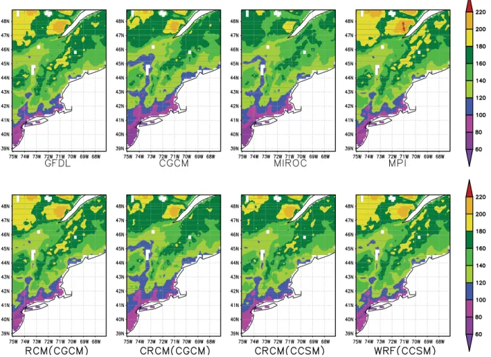
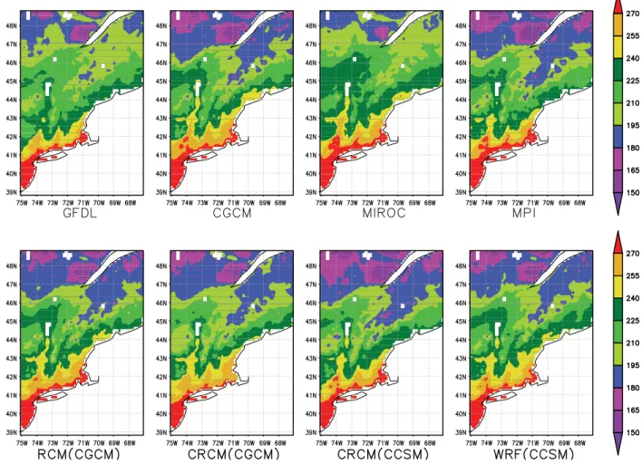
The 20-year (2046_–2065) mean of_five extreme indicators (de-fined inTable 1) were calculated for the northeast US using spatially downscaled and bias corrected data from different GCM and RCM simulations. The indicators were also estimated based on observation for the period of 1976–1995 and the predicted changes were defined as the differences between bias corrected model predictions for 2046–2065 and present-day observations (1976–1995), averaged among GCMs and RCMs respectively. After bias correction, both the magnitude and spatial pattern of Fd in future climate predicted by all GCMs and RCMs are very similar to one another, with a larger number of frost days for inland than coastal areas (Fig. 4). Similarly, bias correction of model outputs leads to a higher level of agreements among the models in predicting both the magnitude and spatial pat-tern of the future mean GSL (Fig. 5). Because of the warmer temper-ature along the coastal areas, the mean growing season is longer as compared to that in inland areas. Similarly, the growing season length is found to be longer in lower latitudes, which is consistent with tem-perature gradient. Because of the decrease in mean temtem-perature from

coastal to inland areas, a spatial trend for later greenup occurrence (as re_flected by the higher values of TGO) further away from the coast or at higher latitudes is predicted by all the models (Fig. 6). The high values of spatial correlation coefficient between each individual model and the multi-model average (GCM and RCM separately) for tem-perature extremes indicate that the SDBC method has been successful in reducing the variability among the outputs from different models and thus reduces the uncertainties related to their use in regional impact studies (Table 4).

The differences between the future mean (2046–2065, based on the bias-corrected and downscaled GCM and RCM ensembles) and the observed mean of the present-day climate (1976–1995) reflect the predicted changes in extreme temperature events in the future climate (Fig. 7). All models predict a decrease in the future mean of Fd because of the warming of the climate. The decrease ranges from 27 to 36 days for most of the area in the northeast US, with the de-crease predicted by the GCM ensemble being slightly larger in magni-tude than the RCM ensemble. Mean GSL will increase because the growing season will start earlier and end later in the warmer future climate. This increase tends to be greater in higher latitudes based on the GCM ensemble, and is relatively uniform in the RCM ensemble (ranging from 15 to 25 days for the entire northeast US). As GDD re-quired for leaf out will be met earlier in a warmer climate, an advance in the greenup onset is predicted by both model ensembles. This ad-vance is faster in the coastal areas than inland areas, and this spatial contrast is stronger in the RCM ensemble than the GCM ensemble.

Except for the WRFG–CCSM, the 20-year (2046–2065) mean values for R10 derived from the bias corrected and downscaled

GCM and RCM outputs agree well, with more frequent heavy precip-itation events occurring in the coastal area (Fig. 8). Despite bias cor-rection, WRFG–CCSM deviates from other models with overall lower values, especially along the coast where it predicts a decrease in R10 as compared to the present-day mean. This is due to the signal from the raw WRFG–CCSM output which predicts a decrease in heavy precipitation events in future climate. Bias corrected model outputs also show some variability in predicting the future mean (2046–2065) for R5d. However, majority of the models capture

similar spatial pattern, with higher values along the coastal area and lower further inland, especially in the northeastern part of the region (Fig. 9). Compared to R10, the larger disparity between individual model and the multi-model average for R5d leads to the lower spatial correlation coefficient for both ensembles (Table 4). Differences be-tween future mean and present-day (1976–1995) observed mean of the extreme precipitation indices show the future changes in extreme precipitation events (Fig. 10). Almost the entire region is projected to experience an increase, albeit small, in the number of days per annum with precipitation greater than 10 mm. The GCM and RCM ensem-bles, both indicating a decrease for some areas in the northeast US, show larger disparity in predicting changes in maximum 5-day total precipitation.

One of the objectives of our study was to investigate whether in-corporating dynamic downscaling by RCM as an intermediate step (i.e., dynamic downscaling of GCM output followed by statistical downscaling of RCM output) can impact thefinal results (compared with statistical downscaling directly from GCM output). In order to test the significance of the impact of dynamic downscaling, variances of the mean values of each extreme indicator obtained from GCM–

SDBC approach were compared with those from GCM–RCM–SDBC ap-proach. Levene's Test was performed to analyze the equality of vari-ances from two groups.Table 5shows the spatially averaged values of Levene's Test statistic. The groups were so chosen to maximize the possibility of getting largest variances between two groups. In all cases, the values of Levene's Tests statistic are less than the critical F-value at 10% level of significance. Therefore, including RCMs as an intermediate step does not considerably reduce (or increase) the

Fig. 6.Future mean (2046–2065) of time for greenup onset (Julian day) from spatially downscaled and bias corrected GCM and RCM simulations.

Table 4

Spatial correlation coefficient between each individual model and the multi-model av-erage (GCM and RCM separately) in predicting temperature and precipitation ex-tremes after statistical downscaling and bias correction.

Model Spatial correlation coefficient with model average

Fd GSL TGO R5d R10

GFDL 0.997 0.989 0.986 0.823 0.984

CGCM 0.998 0.989 0.997 0.823 0.969

MPI 0.999 0.996 0.998 0.776 0.987

MIROC 0.995 0.995 0.995 0.773 0.958

PCM N/A N/A N/A 0.79 0.945

CCSM N/A N/A N/A 0.763 0.972

RCM–CGCM 0.998 0.997 0.998 0.655 0.983

CRCM–CCSM 0.998 0.998 0.999 N/A N/A

CRCM–CGCM 0.994 0.995 0.999 0.746 0.981

WRFG–CCSM 0.997 0.996 0.998 0.708 0.932

disagreement among the models in their future projections of the cli-mate extremes.

4. Summary and conclusion

The BCSD method ofWood et al. (2002)was modified to develop the SDBC approach to process daily outputs from GCMs and RCMs, which results in a multi-model dataset of bias corrected and

downscaled daily maximum and minimum temperature and precipi-tation for the period of 2046–2065 at a spatial resolution of 1∕8° × 1∕8°.

Using the bias corrected and downscaled dataset developed from GCM and RCM simulations for the A2 emission scenario, three temperature-related and two precipitation-related extreme indicators were analyzed for the northeast US. After the spatial downscaling and bias correction, the agreement among the GCM and RCM outputs increased in predicting extreme events in the future climate. The

incorporation of dynamic downscaling by RCMs prior to the statistical downscaling did not cause any significant changes in the prediction of temperature and precipitation extremes in future climate. This implies that statistical downscaling with bias correction is an effective tool to derive fine resolution predictions directly from coarse resolution GCMs' outputs. However, the skill of the downscaling procedure largely depends on the scope of the study. For process-based studies (e.g., in studies on the interaction between different climatic variables or the feedback between different component of the regional climate system; Alo and Wang, 2010), statistical downscaling may not be appropriate and dynamic downscaling will be the choice.

In order to quantify the future changes in extreme events, future predictions from GCM and RCM ensembles were compared against

present-day observations. Results from the ensembles of six GCMs and four RCMs might not be sufficient in completely addressing the uncertainty in model predictions. Including only one emission scenar-io is another limitatscenar-ion related to the predictscenar-ion of climate extremes presented in this study. Also not captured is the uncertainties related to possible absence of low-frequency natural variability in the histor-ical record or model hindcast. However, robust characterization of uncertainty in climate prediction is beyond the scope of our study and the analysis of future changes in the climate extremes is included as an illustration of the applicability offine-scale daily climate dataset developed here in regional climate impact studies. Based on the re-sults of this study, the total number of frost days is projected to decrease in the future due to warming, and the magnitude of the

decrease will be fairly uniform across most of the northeast US. In a warmer climate, the accumulated growing degree days required for leaf greenup will be met earlier causing an earlier greenup onset, while the earlier arrival of spring and delayed fall will lead to an ex-tended growing season. Analysis of precipitation extremes indicates that the number of days with precipitation greater than 10 mm is projected to increase in the northeast US, although in some parts of the region a decrease in the amount of maximum 5-day total precip-itation is projected.

The SDBC method, similar to other statistical downscaling ap-proaches based on probability mapping, retains the large-scale climate change signal predicted by the GCM or RCM. The bias correction implemented as part of the statistical downscaling method potentially offsets the added value of regional climate simulation using a RCM

(which generally performs better than GCMs in simulating regional climate). However, its main contribution is to produce a future value for the climate variable of interest at high resolution, with model bias corrected. The resultingfine-scale climate data provides a more credible future forcing for impact assessment models, which takes the future climate itself as the input (as opposed to the predicted change). This is especially important in the case of nonlinear processes/responses to climate changes.

Acknowledgments

This work was supported by funding from the USDA-NRI (grant no. 2008-003237), the University of Connecticut Center for Environ-mental Sciences and Engineering (CESE), and NSF (AGS-1049017).

References

Abatzoglou, J.T., Brown, T.J., 2011. A comparison of statistical downscaling methods suited for wildfire applications. International Journal of Climatology.http://dx.doi.org/ 10.1002/joc.2312.

Alexander, L.V., Zhang, X., Peterson, T.C., Caesar, J., Gleason, B., Klein Tank, A.M.G., Haylock, M., et al., 2006. Global observed changes in daily climate extremes of tem-perature and precipitation. Journal of Geophysical Research 111 (D5), 1–22.http:// dx.doi.org/10.1029/2005JD006290.

Alo, C.A., Wang, G., 2010. Role of dynamic vegetation in regional climate predictions over Western Africa. Climate Dynamics 35 (5), 907–922.

Boé, J., Terray, L., Habets, F., Martin, E., 2006. A simple statistical-dynamical downscal-ing scheme based on weather types and conditional resampldownscal-ing. Journal of Geophysical Research 111, D23106.http://dx.doi.org/10.1029/2005JD006889. Chen, S.-C., Roads, J.O., Juang, H.-M.H., Kanamitsu, M., 1999. Global to regional

simula-tions of California wintertime precipitation. Journal of Geophysical Research 104 (D24), 31,517–31,532.http://dx.doi.org/10.1029/1998JD200043.

Christensen, Ole B., Christensen, Jens H., Machenhauer, Bennert, Botzet, Michael, 1998. Very high-resolution regional climate simulations over Scandinavia—present cli-mate. Journal of Climate 11, 3204–3229.

Dettinger, M.D., Cayan, D.R., Meyer, M.K., Jeton, A.E., 2004. Simulated hydrologic re-sponses to climate variations and change in the Merced, Carson, and American River basins, Sierra Nevada, California, 1900–2099. Climate Change 62, 283–317. Feddersen, H., Andersen, U., 2004. A method for statistical downscaling of seasonal

en-semble predictions. Tellus Series A 57, 398–408. http://dx.doi.org/10.1111/j.1600-0870.2005.00102.x.

Foley, J.A., Prentice, I.C., Ramankutty, N., Levis, S., Pollard, D., Sitch, S., Haxeltine, A., 1996. An integrated biosphere model of land surface processes, terrestrial carbon balance, and vegetation dynamics. Global Biogeochemical Cycles 10 (4), 603–628. Frich, P., Alexander, L.V., Della-Marta, P., Gleason, B., Haylock, M., Klein Tank, A., Peterson, T., 2002. Observed coherent changes in climatic extremes during the sec-ond half of the twentieth century. Climate Research 19, 193–212.http://dx.doi.org/ 10.3354/cr019193.

Giorgi, F., Mearns, L.O., 1991. Approaches to the simulation of regional climate change: a review. Reviews of Geophysics 29 (2), 191–216.http://dx.doi.org/10.1029/ 90RG02636.

Hayhoe, Katharine, Wake, C.P., Huntington, T.G., Luo, L., Schwartz, M.D., Sheffield, J., Wood, E., et al., 2006. Past and future changes in climate and hydrological indica-tors in the US Northeast. Climate Dynamics 28 (4), 381–407.http://dx.doi.org/ 10.1007/s00382-006-0187-8.

Iizumi, T., Nishimori, M., Dairaku, K., Adachi, S.A., Yokozawa, M., 2011. Evaluation and intercomparison of downscaled daily precipitation indices over Japan in present-day climate: strengths and weaknesses of dynamical and bias correction-type sta-tistical downscaling methods. Journal of Geophysical Research 116 (D1), 1–20. http://dx.doi.org/10.1029/2010JD014513.

Kidson, J.W., Thompson, C.S., 1998. A comparison of statistical and model-based down-scaling techniques for estimating local climate variations. Journal of Climate 11, 735–753.http://dx.doi.org/10.1175/1520-0442(1998)011b0735:ACOSAM>2.0.CO;2. Kiktev, D., Sexton, D.M.H., Alexander, L., Folland, C.K., 2003. Comparison of modeled and ob-served trends in indices of daily climate extremes. Journal of Climate 16, 3560–3571. http://dx.doi.org/10.1175/1520-0442(2003)016b3560:COMAOT>2.0.CO;2. Kucharik, C.J., Foley, J.A., Delire, C., Fisher, V.A., Coe, M.T., Lenters, J.D., Young-Molling,

C., et al., 2000. Testing the performance of a dynamic global ecosystem model: water balance, carbon balance, and vegetation structure. Global Biogeochemical Cycles 14 (3), 795.http://dx.doi.org/10.1029/1999GB001138.

Li, H., Sheffield, J., Wood, E.F., 2010. Bias correction of monthly precipitation and tem-peraturefields from Intergovernmental Panel on Climate Change AR4 models

Fig. 10.Present-day mean (1976–1995) and predicted change for extreme precipitation indicators, based on the GCM and RCM ensemble in future climate (2046–2065).

Table 5

Spatially average values of Levene's test statistics to test the equality of variances in the results obtained from GCM–BCSD approach and GCM–RCM–BCSD approach. At 10% level of significance, for the respective degrees of freedom, the critical F-value is 4.54.

GCM GCM–RCM Extreme index Levene's test statistic GFDL, CGCM, CCSM CRCM–CGCM, WRFG–CCSM, RCM–GFDL R10 3.75 R5d 3.07 GFDL, CGCM, MPI RCM–CGCM, CRCM–CGCM, WRFG–CCSM Fd 0.84 GSL 3.17 TGO 1.66

using equidistant quantile matching. Journal of Geophysical Research 115, D10101. http://dx.doi.org/10.1029/2009JD012882.

Marinucci, M.R., Giorgi, F., 1992. A 2XCO2climate change scenario over europe gener-ated using a limited area model nested in a general circulation model 1. Present-day seasonal climate simulation. Journal of Geophysical Research 97 (D9), 9989–10,009.http://dx.doi.org/10.1029/92JD00615.

Maurer, E.P., 2007. Uncertainty in hydrologic impacts of climate change in the Sierra Nevada, California under two emissions scenarios. Climatic Change 82 (3–4), 309–325.http://dx.doi.org/10.1007/s10584-006-9180-9.

Maurer, E.P., Hidalgo, H.G., 2008. Utility of daily vs. monthly large-scale climate data: an intercomparison of two statistical downscaling methods. Hydrology and Earth System Sciences 12, 551–563.

Maurer, E.P., Wood, A.W., Adam, J.C., Lettenmaier, D.P., Nijssen, B., 2002. A long-term hydrologically-based data set of land surfacefluxes and states for the contermi-nous United States. Journal of Climate 15 (22), 3237–3251.

Maurer, E.P., Hidalgo, H.G., Das, T., Dettinger, M.D., Cayan, D.R., 2010. The utility of daily large-scale climate data in the assessment of climate change impacts on daily streamflow in California. Hydrology and Earth System Sciences 14, 1125–1138. http://dx.doi.org/10.5194/hess-14-1125-2010.

Murphy, J., 1999. An evaluation of statistical and dynamical techniques for downscaling local climate. Journal of Climate 12 (8), 2256–2284.

Noguer, M., Jones, R., Murphy, J., 1998. Sources of systematic errors in the climatology ofa regional climate model over Europe. Climate Dynamics 14, 691–712. Orlowsky, B., Seneviratne, S.I., 2011. Global changes in extreme events: regional and

sea-sonal dimension. Climatic Change.http://dx.doi.org/10.1007/s10584-011-0122-9. Payne, J.T., Wood, A.W., Hamlet, A.F., Palmer, R.N., Lettenmaier, Dennis P., 2004. Mitigating

the effects of climate change on the water resources of the Columbia River Basin. Climat-ic Change 62 (1–3), 233–256.http://dx.doi.org/10.1023/B:CLIM.0000013694.18154.d6. Schmidli, J., Frei, C., Vidale, P.L., 2006. Downscaling from GCM precipitation: a bench-mark for dynamical and statistical downscaling methods. International Journal of Climatology 26 (5), 679–689.http://dx.doi.org/10.1002/joc.1287.

Shepard, D., 1968. A two-dimensional interpolation function for irregularly-spaced data. Proceedings of the 1968 23rd ACM national conference on. ACM Press, New York, New York, USA, pp. 517–524.http://dx.doi.org/10.1145/800186.810616. Tebaldi, C., Hayhoe, Katharinec, Arblaster, J.M., Meehl, G.A., 2006. Going to the

ex-tremes. Climatic Change 79 (3–4), 185–211. http://dx.doi.org/10.1007/s10584-006-9051-4.

VanRheenen, N.T., Wood, A.W., Palmer, R.N., Lettenmaier, Dennis P., 2004. Potential Implications of PCM climate change scenarios for Sacramento–San Joaquin river basin hydrology and water resources. Climatic Change 62 (1–3), 257–281.http:// dx.doi.org/10.1023/B:CLIM.0000013686.97342.55.

Widmann, M.L., Bretherton, C.S., Salath´e Jr., E.P., 2003. Statistical precipitation down-scaling over the Northwestern United States using numerically simulated precipi-tation as a predictor. Journal of Climate 16, 799–816.

Wilby, R.L., Wigley, T.M.L., 2000. Precipitation predictors for downscaling: observed and general circulation model relationships. International Journal of Climatology 20, 641–661.

Wilby, R.L., Wigley, T.M.L., Conway, D., Jones, P.D., Hewistson, B.C., Main, J., Wilks, D.S., 1998. Statistical downscaling of general circulation model output: a comparison of methods. Water Resources Research 34, 2995–3008.

Wilby, R.L., Hay, L.E., Gutowski Jr., W.J., Arritt, R.W., Takle, E.S., Pan, Z., Leavesley, G.H., Clark, M.P., 2000. Hydrological responses to dynamically and statistically down-scaled climate model output. Geophysical Research Letters 27, 1199–1202. Wood, A.W., Maurer, E.P., Kumar, A., Lettenmaier, D.P., 2002. Long-range experimental

hydrologic forecasting for the eastern United States. Journal of Geophysical Re-search 107 (D20), 4429.http://dx.doi.org/10.1029/2001JD000659.

Wood, A.W., Leung, L.R., Sridhar, V., Lettenmaier, D.P., 2004. Hydrologic implications of dynamical and statistical approaches to downscaling climate model outputs. Climatic Change 62, 189–216.

Zorita, E., von Storch, H., 1999. The analog method as a simple statistical downscaling technique: comparison with more complicated methods. Journal of Climate 12, 2474–2489.http://dx.doi.org/10.1175/1520-0442.