Kernel Methods for Learning with Limited Labeled Data

(1)

Kernel Methods for Learning with Limited Labeled Data

by

Aniket Anand Deshmukh

A dissertation submitted in partial fulfillment

of the requirements for the degree of

Doctor of Philosophy

(Electrical and Computer Engineering)

in The University of Michigan

2019

Doctoral Committee:

Associate Professor Clayton Scott, Chair

Professor Alfred O. Hero, III

Assistant Professor Eric Schwartz

Associate Professor Ambuj Tewari

(2)

Aniket Anand Deshmukh

[email protected]

ORCID iD: 0000-0002-7292-8436

(3)

(4)

ACKNOWLEDGEMENTS

I would like to begin my thesis by thanking several mentors and friends who made this thesis possible. First, I would like to thank my advisor Prof. Scott with whom I worked for last five years. Prof. Scott has been an inspiration to me right from the start of my doctoral program. Prof. Scott was patient with me, and whenever I did not understand anything, he would start from very simple ideas and using them explain me the complex ones. During the last five years, we have had long sessions discussing proofs and brainstorming ideas. I am thankful to Prof. Scott for giving me a chance to work with him and investing many subsequent hours on me. Prof. Scott’s openness to new ideas helped me think independently. Prof. Scott is very particular about thoroughness and depth of research in hand. He also helped me improve my writing and communication skills. I thank Prof. Scott for making me a good machine learning researcher, and I will always strive to do thorough research in the future.

I thank the committee members for timely feedback and giving me suggestions whenever I needed them. I thank Prof. Ambuj Tewari for helping me solve some of the queries I had about contextual bandits at the start of my research. His course - “Sequential Decision Making with mHealth Applications" boosted my research in the area of bandits. I also thank Prof. Eric Schwartz for helpful discussions on best arm identification. Prof. Eric helped me understand real-world applications of bandits. Prof. Alfred Hero’s work in the area of sensor network has been helpful for me to understand the best sensor selection problem.

(5)

Michigan. To Becky Turanski, José-Antonio Rubio, Anne Rhoades, Karen Liska, Kristen Thornton, Amy Wicklund, and Judi Jones: thank you for helping me.

I would also like to thank my undergraduate professors at IIT Hyderabad, Prof. K Sri Rama Murty, Prof. Sumohana Channappayya, Prof. Soumya Jana, Prof. Balasubramaniam Jayaram and Prof. Mohammed Zafar Ali Khan for encouraging me to apply for PhD and instilling research ideology in me early in my undergraduate studies.

Next, I would like to thank Dr. Urun Dogan for the collaboration and his immense help in formulating problems during my PhD. Urun’s enthusiasm for innovation in machine learning research and discussions with him on research papers have helped me understand fundamental challenges in machine learning.

I was introduced to online learning and bandits by Prof. Jacob Abernethy in his course “Theoretical Foundations of Machine Learning" in the second year of my PhD. I thank Jake for motivating me to explore the area of bandits. I thank Prof. Raj Rao Nadakuditi, Prof. Sandeep Pradhan and Prof. Laura Balzano for making my fundamentals stronger through various courses during PhD, which helped me conduct my research better.

I would like to thank my collaborator and friend Srinagesh for working with me during PhD. Discussions on mathematics, machine learning and interdisciplinary work with Srinagesh helped me broaden my horizons.

I thank David Hong and John Lipor for introducing me to new ideas and philosophies during my stay at Ann Arbor. I learned a lot through our exchanges on mathematics and philosophy. I also learned the importance of family and effective time management from John. I thank Matthew Kvalheim for collaborating with me and teaching me nonlinear dynamics and control systems. I also would like to thank Aditya Modi and Julian Katz-Samuels for discussing research areas in bandits and introducing me to new techniques of analyzing bandit algorithms. I thank Vikas Dhiman for studying “Regret Analysis of Stochastic and

(6)

Nonstochastic Multi-Armed Bandit Problems" book with me. Our study sessions helped me understand the proofs of various bandit algorithms. Our exchange of thoughts about the education system, activism has also helped me understand this world better.

I thank Abhishek Bafna, Sri Sharan Banagiri, Arnab Hazari, Niket Prakash, Naveen Murthy, Pragya Agrawal, Poornashree Rajendra and Kalyan Tej for being there for me during my ups and downs. Without all of you, my time at Ann Arbor would have never been so much fun. I had a good time with our dinner parties, political discussions and playing squash & racketball. I thank Abhishek Bafna, Naveen Murthy and Pragya Agrawal for collaborating with me on various course projects and teaching me various concepts during coursework.

I would like to thank Chaitanya Kulkarni, Sachin Rathod and Pravin Shedolkar for fun conversations and supporting me in my ambitions. I thank Omkar for being there for me and helping me during my time at Ann Arbor. I learned how to have fun in life and how to be a good cook from Omkar. Next, I would like to thank Piyush who has been a great support for me during the last 12 years and guided me on most major decisions in life. I would also like to thank Aditya who encouraged me to study speech processing and machine learning during my undergraduate. I have always had great technical discussions with Aditya, and he helped me keep up with the machine learning literature during my PhD.

I would like to thank my girlfriend Mansi for encouraging me during my bad times and supporting me to finish my PhD. This journey has been fun and easier with Mansi in my life. I would also like to thank my uncles Shankar and Dhananjay and my grandfather Dnyanoba for nurturing my interest in Science and Technology. Most importantly I would like to thank my brother Anup and my parents Ratnamala and Anand. Without their constant love, support and guidance, I would not have been able to pursue higher education and complete my PhD.

(7)

LIST OF TABLES

TABLE

1.1 Contribution: Simple regret minimization for contextual bandits . . . 7

2.1 RMSE of Marginal Transfer Learning on Parkinson’s Disease Dataset . . . . 29

2.2 RMSE of Pooling on Parkinson’s Disease Dataset . . . 30

2.3 Average Classification Error of Marginal Transfer Learning on Satellite Dataset 32 2.4 Average Classification Error of Pooling on Satellite Dataset . . . 32

2.5 Average Classification Error of Marginal Transfer Learning on Flow Cytometry Dataset . . . 34

2.6 Average Classification Error of Pooling on Flow Cytometry Dataset . . . 34

2.7 Summary of Multiclass Datasets for Domain Generalization . . . 38

(12)

LIST OF FIGURES

FIGURE

1.1 Multi-armed Bandit Problem . . . 4

1.2 Contextual Bandit Problem . . . 6

2.1 Parkinson’s disease telemonitoring dataset . . . 31

2.2 Satellite dataset . . . 33

2.3 Classification error rates for baseline and proposed method for different exper-imental settings, i.e., number of examples per task and number of tasks. . . 35

2.4 Synthetic Dataset: Three tasksθ = {0,90,180} . . . 39

2.5 Synthetic Dataset: Thirteen tasks θ ={0,15,30, ...,180} . . . 39

2.6 MNIST Data with no rotation (first row) and 90 degree rotation (second row) 40 3.1 Synthetic Data . . . 65

3.2 Results on Multiclass Datasets - Empirical Mean Regret . . . 66

4.1 Scientific measurement: magnetic field lines of the Earth (Credit: NASA/God-dard Scientific Visualization Studio) . . . 93

4.2 TBEx Small Satellite with Multiple Magnetometers [1,2] . . . 95

4.3 Contextual-Gap exploration policy: case 1 . . . 100

4.4 Contextual-Gap exploration policy: case 2 . . . 101

(13)

4.6 Average Simple Regret Evaluation on Spacecraft Magnetic Field Dataset . . 110 4.7 Histogram of Arm Selection during exploration . . . 111 4.8 Worst Case Simple Regret Evaluation on Spacecraft Magnetic Field Dataset 112

(14)

ABSTRACT

Machine learning is a rapidly developing technology that enables a system to automatically learn and improve from experience. Modern machine learning algorithms have achieved state-of-the-art performances on a variety of tasks such as speech recognition [3], image classification [4], machine translation [5], playing games like Go [6], Dota 2 [7], etc. However, one of the biggest challenges in applying these machine learning algorithms in the real world is that they require huge amount of labeled data for the training. In the real world, the amount of labeled training data is often limited.

In this thesis, we address three challenges in learning with limited labeled data using kernel methods. In our first contribution, we provide an efficient way to solve an existing domain generalization algorithm and extend the theoretical analysis to multiclass classification. As a second contribution, we propose a multi-task learning framework for contextual bandit problems. We propose an upper confidence bound-based multi-task learning algorithm for contextual bandits, establish a corresponding regret bound, and interpret this bound to quantify the advantages of learning in the presence of high task (arm) similarity. Our third contribution is to provide a simple regret guarantee (best policy identification) in a contextual bandits setup. Our experiments examine a novel application to adaptive sensor selection for magnetic field estimation in interplanetary spacecraft and demonstrate considerable improvements of our algorithm over algorithms designed to minimize the cumulative regret.

(15)

CHAPTER I

Introduction

Machine learning is a rapidly developing technology and has the potential to solve many issues in speech processing, natural language processing, robotics, autonomous cars, and fields where data analysis is essential. Machine learning enables systems to automatically learn and improve from the experience without manually programming it for every scenario. Modern machine learning algorithms have achieved state-of-the-art performances on variety of tasks such as speech recognition [3], image classification[4], machine translation [5], playing games like Go [6], Dota 2 [7] ,etc. However, one of the biggest challenges in applying these machine learning algorithms in the real world is that they require huge amount of labeled data for the training. In real world, we are limited by the labeled data that’s available during training, and which may also be distributionally different from the test data.

Consider an example of categorizing blood cells of a patient in two types, lymphocytes and non-lymphocytes. Doctors measure various physical and chemical properties of a cell using flow cytometry and then based on these properties, doctors have to manually label each cell into two types. Creating such a labeled dataset for learning algorithm is a very time consuming and expensive process. Also, physical and chemical properties of each blood cell may vary according to patient and that’s why data used during training could

(16)

be distributionally different than test data. One more example where collecting labeled data is very expensive is clinical trials. In clinical trials, doctors have number of options for drugs or type of treatments. Doctors try these options on various patients and check how effective the particular option is; which is equivalent to collecting labeled data or training data. Doctors have to minimize number of trials because trying wrong treatment could have adverse effects on patients. In this case, collecting labeled data is not only expensive but is also life threatening.

I.1 Background

In this section, I describe challenges addressed in the thesis and give necessary background. Specifically, I explore three main scenarios where I address issues that arise due to limited labeled data and solve these issues using kernel methods.

I.1.1 Domain Generalization

Transfer learning, domain adaptation, and weakly supervised learning all have the goal of generalizing without access to conventional labeled training data. One particular form of transfer learning that has garnered increasing attention in recent years isdomain generalization

(DG) [8, 9]. In this setting, the learner is given unlabeled data to classify, and must do so by leveraging labeled data sets from similar yet distinct classification problems. In other words, label training data drawn from the same distribution as the test data are not available, but are available from several related tasks (which may have slightly different distribution). We use the terms “task" and “domain" interchangeably throughout this chapter.

Applications of DG are numerous. For example, each task may be a prediction problem associated to a particular individual (e.g., handwritten digit recognition), and the variation

(17)

between individuals accounts for the variation among the data sets. Domain generalization is needed when a new individual appears, and the only training data come from different subjects.

Consider the example of image classification, where one has images of different objects. Each image contains a single object and the goal is recognize or classify these images based on an object in it. We have multiple images of the same objects from different cameras, and we train our image classification model for these cameras (e.g., Apple’s iPhone, Sony’s DSLR, and Google’s Pixel). During the test time, the goal is to classify images from Samsung’s Note. Different cameras have different optical structure and so images from those cameras may look slightly different or may have different optical properties. What makes this more difficult is that there are no labeled images from Samsung’s Note; and the classification model should be able to classify images from Samsung’s Note without any labeled data.

As another application, we consider domain generalization for determining the orbits of microsatellites, which are increasingly deployed in space missions for a variety of scientific and technological purposes. Because of randomness in the launch process, the orbit of a microsatellite is random, and must be determined after the launch. Furthermore, ground antennae are not able to decode unique identifier signals transmitted by the microsatellites because of communication resource constraints and uncertainty in satellite position and dynamics. More concretely, supposec microsatellites are launched together. Each launch is a random phenomenon and may be viewed as a task in our framework. One can simulate the launch of microsatellites using domain knowledge to generate highly realistic training data (feature vectors of ground antennae RF measurements, and labels of satellite ID). One can then transfer knowledge from the simulated training data to label (identify the satellite) the measurements from a real-world launch with high accuracy.

Domain generalization is the problem of assigning labels to an unlabeled data set, given several similar data sets for which labels have been provided [10]. More specifically, in domain

(18)

generalization, the learning algorithm hasN datasets during training with each dataset drawn from different probability distributions such that each point in each dataset has a label or class associated with it. The goal is to learn a classifier such that, given a new dataset (with no training data/labels) drawn from a different but similar probability distribution, it is possible to provide labels to its points.

I.1.2 Multi-Task Learning for Contextual Bandits

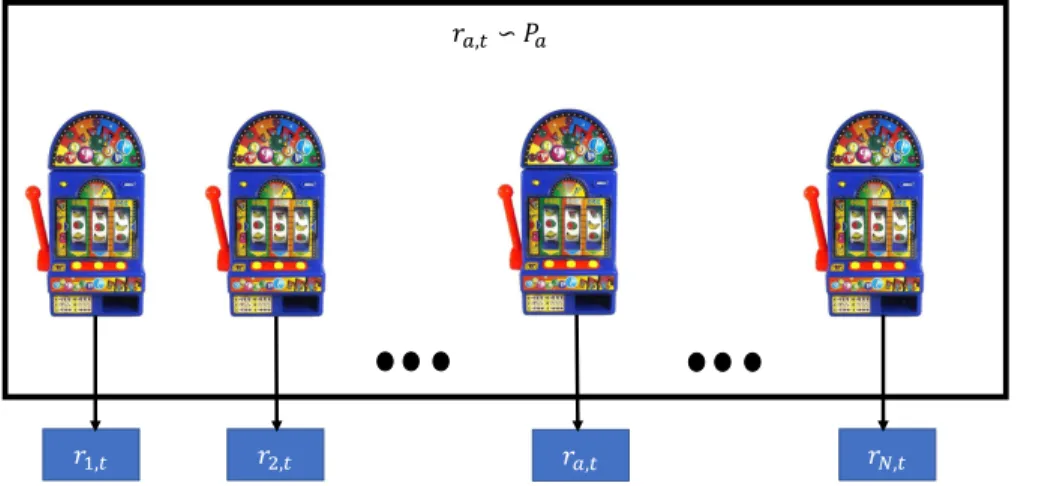
A multi-armed bandit (MAB) problem is a sequential decision-making problem where, at each time step, an agent chooses one of several “arms," and observes high reward for choosing the correct arm and smaller reward if it chooses some other arm. The name "multi-armed bandit" arises from an imaginary gambler who has access to number of slot machines. Slot machines here are also called "one-armed bandits". In order to achieve a goal of maximizing money in hand in certain number of trials, the gambler has to decide how many times to play each machine and in which order to play those machines [11].

𝑟𝑎,𝑡∽ 𝑃𝑎

𝑟𝑁,𝑡

𝑟2,𝑡 𝑟𝑎,𝑡

𝑟1,𝑡

(19)

More formally, the gambler here is called the learner, each slot machine is an arm and the problem of making decision of choosing arms is called the multi-armed bandit (MAB) problem. The “regret" of the learner is the difference between the maximum possible reward and the reward resulting from the chosen action. The reward for each arm is random according to a fixed distribution, and the learner’s goal is to either maximize its cumulative reward or minimize cumulative regret [12] through a combination of exploring different arms and exploiting those arms that have yielded high rewards in the past [13,14]. For example, in Fig. 1.1, there areN arms to choose from, rewardra,t for each arma at timet is sampled

from a probability distribution Pa. In this case, the goal is to minimize cumulative regret

RT =max a∈[N] T X t=1 ra,t − T X t=1

rat,t, where [N]=1, ...,N, at is the arm selected by a learner at time t andT are number of trials. If the learner explores too little, it may never find an optimal arm, which will in consequence increase its cumulative regret. If the learner explores too much, it may select sub-optimal arms too often which will also increase its cumulative regret.

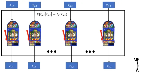
The contextual bandit problem is an extension of the MAB problem where there is some side information, here called the context, associated with each arm [15]. The contextual bandit setting is also called associative reinforcement learning [16] and linear bandits [17,18]. In Fig. 1.2, there is a context xa,t for an arma at timet. The expected reward for each arma given

a contextx_a,t is some fixed but unknown function ofxa,t. More formally, E[rat,t|xa,t]= fa(xa,t). Contextual bandits have been used to model personalized news recommendations, ad placements, and other applications. Each context determines the distribution of rewards for the associated arm. The goal, therefore, in contextual bandits is still to maximize the cumulative reward or minimize cumulative regret, but now leveraging the contexts to predict the expected reward of each arm. i.e. RT =

T X t=1 ra∗ t,t − T X t=1 rat,t, where a ∗

t is the arm with

maximum reward at trial t. Note that arm with maximum reward in contextual bandits depends on the context unlike in MAB. Contextual bandits have been employed to model various applications like news article recommendations [19], computational advertisements

(20)

[20], website optimization [21] and clinical trials [22]. For example, in the case of a news article recommendation, the agent must select a news article to recommend to a particular user. The arms are articles, and contextual features are features derived from the article and the user. The reward is based on whether a user reads the recommended article.

𝑟𝐾,𝑡

𝑟2,𝑡 𝑟𝑎,𝑡

𝑟1,𝑡

𝐸[𝑟𝑎,𝑡𝑥𝑎,𝑡 = 𝑓𝑎(𝑥𝑎,𝑡)

𝑥1,𝑡 𝑥2,𝑡 𝑥𝑎,𝑡 𝑥𝐾,𝑡

Figure 1.2: Contextual Bandit Problem

One common approach to contextual bandits is to fix the class of policy functions (i.e., functions from contexts to rewards) and try to learn the best function with time [23, 24,25]. Most algorithms estimate rewards either separately for each arm or have one single estimator that is applied to all arms. But when rewards are estimated separately for each arm, we may be exploring more because arms could be similar to each other and if rewards are estimated together then we are assuming that there is a single estimator. Both these approaches are at one extreme and in reality arms could be similar to each other to a different extent. Therefore, I use an approach which adopts the perspective of multi-task learning (MTL) where separate estimators or one single estimator are special cases. The intuition is that some arms may be similar to each other, in which case it should be possible to pool the historical data for these arms to estimate the mapping from context to rewards more rapidly. For example, in the case of news article recommendations, there may be thousands of articles, and some of

(21)

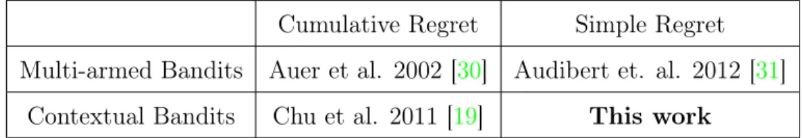
Cumulative Regret Simple Regret Multi-armed Bandits Auer et al. 2002 [30] Audibert et. al. 2012 [31]

Contextual Bandits Chu et al. 2011 [19] This work

Table 1.1: Contribution: Simple regret minimization for contextual bandits

those are bound to be similar to each other. In this case, when news article are similar to each other, we could benefit from estimating their rewards together and we may not need to explore too much to estimate their rewards.

I.1.3 Simple Regret for Contextual Bandits

The previous sub-section has discussed cumulative regret minimization in MAB and contextual bandit. In classical MABs, the goal of the learner is not always to minimize the cumulative regret. In some applications, there is a pure exploration phase during which the learning incurs no regret (i.e., no penalty for sub-optimal decisions), and performance is measured in terms of simple regret, which is the regret assessed at the end of the pure exploration phase. For example, in the best arm identification, the learner must guess the arm with a highest expected reward at the end of the exploration phase. Simple regret minimization clearly motivates different strategies, since there is no penalty for sub-optimal decisions during the exploration phase. Fixed budget and fixed confidence are the two main theoretical frameworks in which simple regret is generally analyzed [26, 27, 28, 29]. The number of trials for the exploration are fixed in the fixed budget setting and the goal is to maximize the probability of returning the best arm. In the fixed confidence setting, the goal is to achieve a fixed confidence about the quality of the returned arm in minimum possible number of trials. [26].

To date, work on contextual bandits has studied cumulative regret minimization i.e.

T X t=1 ra∗ t,t − T X t=1

rat,t, which is motivated by applications in healthcare, web advertisement recommendations and news article recommendations [23]. In this thesis, I extend the idea of

(22)

simple regret minimization to contextual bandits i.e. minimizing the regret at time t > T (after exploration phase)ra∗

t,t −rat,t. In this setting, there is a pure exploration phase during which no regret is incurred, followed by a pure exploitation phase during which regret is incurred, but there is no feedback so the learner cannot update its policy. To my knowledge, previous work has not addressed novel algorithms for this setting.

I.2 Contribution

The three major contributions of this thesis are summarized below.

1. Domain Generalization: In my first contribution (see chapter 2), I provide an efficient way to solve an existing kernel based domain generalization and extend the theoretical analysis to the multi-class classification. To be specific, I propose a kernel approximation technique which reduces the time complexity of the solver in the existing kernel based domain generalization approach to linear in terms of the number of samples. I give empirical evidence based on two medical datasets and one satellite dataset demonstrating the superiority of these algorithms over state-of-the-art ones. This work was done in collaboration with my advisor Prof. Clayton Scott, Prof. Gilles Blanchard and Dr. Urun Dogan at Microsoft Research.

2. Multi-Task Learning for Contextual Bandits: In chapter 3, I propose an upper confi-dence bound-based multi-task learning algorithm for contextual bandits, establish a corresponding regret bound, and interpret this bound to quantify the advantages of learning in the presence of high task (arm) similarity. I also describe an effective scheme for estimating task similarity from data and demonstrate my algorithm’s performance using several data sets. This work was done in collaboration with Dr. Urun Dogan at Microsoft Research and my advisor Prof. Clayton Scott.

(23)

3. Simple Regret for Contextual Bandits: In chapter 4, I formulate a novel problem: that of simple regret minimization for contextual bandits and develop an algorithm, Contextual-Gap, for this setting. I present performance guarantees on the simple regret in the fixed budget framework and present experimental results for adaptive sensor selection in nano-satellites. This work was done in collaboration with Dr. Srinagesh Sharma, my advisor Prof. Clayton Scott, Prof. James Cutler and Prof. Mark Moldwin.

(24)

CHAPTER II

Domain Generalization

We consider the problem of assigning class labels to an unlabeled test data set, given several labeled training data sets drawn from similar distributions. This problem arises in several applications where data distributions fluctuate because of biological, technical, or other sources of variation. [32] has developed a distribution-free, kernel-based approach to the problem. This approach involves identifying an appropriate reproducing kernel Hilbert space and optimizing a regularized empirical risk over the space. But as dataset size increases, computational complexity of the SVM solver can be quadratic or cubic in terms of number of samples. We propose a kernel approximation technique which reduces the time complexity of the solver to linear in terms of number of samples. Kernel methods project input data points into high dimensional feature space (infinite-dimensional in case of Gaussian kernel) and find the optimal hyperplane in that feature space. Using kernel approximation techniques such as random Fourier features we map the input data to a randomized low-dimensional feature space and then apply existing fast linear SVM solvers. Experimental results are shown on three real world datasets. We also extend the generalization error analysis in [32] for the multi class setting and show supporting experimental results.

(25)

II.1

Introduction

Is it possible to leverage the solution of one classification problem to solve another? This is a question that has received increasing attention in recent years from the machine learning com-munity, and has been studied in a variety of settings, including multi-task learning, covariate shift, and transfer learning. In this work, we study domain generalization, another setting in which this question arises, and one that incorporates elements of the three aforementioned settings, and is motivated by many practical applications.

To state the problem, let X be a feature space andY a space of labels to predict. For a given distribution PXY, we refer to the X marginal distribution PX as simply the marginal

distribution, and the conditionalP_XY(Y|X) as the posterior distribution. There are N similar but distinct distributionsP_XY(i) on X × Y,i =1, . . . ,N. For each i, there is a training sample

Si = (Xij,Yij)1≤j≤ni of i.i.d. realizations of P_XY(i). There is also a test distribution PTXY that

is similar to but again distinct from the “training distributions" P_XY(i). Finally, there is a test sample (XT_j ,Y_jT)1≤j≤nT of i.i.d. realizations ofPXYT , but in this case the labelsYj are not

observed. The goal of domain generalization is to correctly predict these unobserved labels. Essentially, given a random sample from the marginal test distributionP_XT, we would like to predict the corresponding labels.

The goal is to predict these unobserved labels corresponding to samples drawn from the marginal test distribution. One of the methods to solve the transfer learning problem in the above setting is described in [32]. Their approach, marginal transfer learning, is a distribution-free, kernel-based and it involves identifying an appropriate reproducing kernel Hilbert space (RKHS) and optimizing a regularized empirical risk over the space. But as dataset size increases, computational complexity of this solver can be quadratic or cubic in terms of number of samples. We propose a kernel approximation to solve marginal transfer learning in linear time.

(26)

II.2

Motivating Application: Automatic Gating of Flow

Cytometry Data

Flow cytometry is a high-throughput measurement platform that is an important clinical tool for the diagnosis of many blood-related pathologies. This technology allows for quantitative analysis of individual cells from a given population, derived for example from a blood sample from a patient. We may think of a flow cytometry data set as a set ofd-dimensional attribute vectors (X_j)1≤j≤n, where n is the number of cells analyzed, andd is the number of attributes recorded per cell. These attributes pertain to various physical and chemical properties of the cell. Thus, a flow cytometry data set is a random sample from a patient-specific distribution.

Now suppose a pathologist needs to analyze a new (test) patient with data (XT_j )1≤j≤nT. Before proceeding, the pathologist first needs the data set to be “purified" so that only cells of a certain type are present. For example, lymphocytes are known to be relevant for the diagnosis of leukemia, whereas non-lymphocytes may potentially confound the analysis. In other words, it is necessary to determine the labelYT

j ∈{−1,1}associated to each cell, where

Y_jT =1 indicates that the j-th cell is of the desired type.

In clinical practice this is accomplished through a manual process known as “gating." The data are visualized through a sequence of two-dimensional scatter plots, where at each stage a line segment or polygon is manually drawn to eliminate a portion of the unwanted cells. Because of the variability in flow cytometry data, this process is difficult to quantify in terms of a small subset of simple rules. Instead, it requires domain-specific knowledge and iterative refinement. Modern clinical laboratories routinely see dozens of cases per day, so it would be desirable to automate this process.

Since clinical laboratories maintain historical databases, we can assume access to a number (N) of historical patients that have already been expert-gated. Because of biological and

(27)

technical variations in flow cytometry data, the distributionsP_XYi of the historical patients will vary. But every cell type of interest has a known tendency (e.g., high or low) for most measured attributes. Therefore, it is reasonable to assume that there is an underlying distribution (on distributions) governing flow cytometry data sets, that produces roughly similar distributions thereby making possible the automation of the gating process [32].

II.3

Formal Setting

As described in the last section let X be feature space andY be the label space or output space. Further assume that we have samples from N distributions Si = (Xij,Yij)1≤j≤ni. For simplicity assume thatni =n. LetPX×Y be the set of probability distributions on X × Y, PX the set of probability distributions on X, and PY |X the set of conditional probabilities ofY givenX. Further, it is assumed that there exists a distributionµ on P_X×Y, whereP_XY1 , ...,P_XYN are i.i.d. realizations from µ and as already described, samples Si are i.i.d. realizations of

(X,Y) following the distribution Pi XY.

Suppose the user has training samplesSi = ((Xij,Yij))1≤j≤n. Each data pointXij along with its distributionP_Xi can be thought of as an extended data point_X˜_ij ₌ _(Pi

X,Xij) Now, consider

a test sampleST = ((XT_j ,Y_jT))1≤j≤nT, whose labels are not observed by a user. The goal here is to predictY_jT as accurately as possible. A decision function is a function f :PX× X →R (i.e. a classifier on extended feature space) that predicts_Yˆ_j ₌ _f₍_Pˆ_X_,_X_j₎_{, where}_Pˆ_X _{is the associated}

empirical distribution. Let ` :R× Y → R₊ be the appropriate loss used, then the average

loss incurred on the test sample is

L= _n1 T nT X j=1 `(_Yˆ_j_,_Y_j_). _(2.1)

(28)

Based on this the empirical error on test sample with sample sizenT is ˆ ε(f,n_T) = _T1 nT X i=1 `(f(_PˆT X,XTi ),YiT), (2.2)

and the generalization error of a decision function with respect to loss ` is

ε(f) =E_PT

X Y∼µE(XT,YT)∼PTX Y`(f(P

T

X,XT),YT). (2.3)

Denoting_X˜ ₌ _(P_X_,_X₎_{, the above can be written as}

ε(f) =E_PT

X Y∼µE(XT,YT)∼PTX Y`(f(

˜

XT),YT). (2.4)

Important points to note here are:

• At training time as well as at test time, the marginal distribution PX for a sample is

only known through the sample itself, that is, through the empirical marginal _Pˆ_X_,

• Despite the similarity to standard binary classification in the infinite sample case, the learning task here is different, because the realizations (_X˜_ij_,_Y_ij₎ _{are neither independent}

nor identically distributed

II.4

Learning Algorithm

We consider an approach based on kernels. The functionk :Ω×Ω → R is called a kernel on

Ω if the matrix (k(xi,xj))1≤i,j≤n is symmetric and positive semi-definite for all positive integers n and allx1, . . . ,xn ∈ Ω. It is well-known that ifk is a kernel on Ω, then there exists a Hilbert

space_H˜ _and_Φ˜ _:_Ω _→ _H˜ _{such that}_k_(x,_x0₎ ₌_h_Φ(x_˜ _),_Φ(x_˜ 0₎_i

˜

H. WhileH˜ andΦ˜ are not uniquely determined by k, the Hilbert space of functions (from Ω toR)H_k ={hv,Φ(˜ ·)i_H_˜ :v ∈H˜}is

(29)

uniquely determined by k, and is called the reproducing kernel Hilbert space (RKHS) ofk.

One way to envision H_k is as follows. Define Φ(x) :=k(·,x), which is called the canonical

feature map associated with k. Then the span of {Φ(x) : x ∈ Ω}, endowed with the inner

product Φ(x),Φ(x0) = k(x,x0), is dense in _H

k. We also recall the reproducing property,

which states that hf,Φ(x)i= f(x) for all f ∈ H_k.

Several well-known learning algorithms, such as support vector machines and kernel ridge regression, may be viewed as minimizers of a norm-regularized empirical risk over the RKHS of a kernel. A similar development has also been made for multi-task learning [33]. Inspired by this framework, we consider a general kernel algorithm as follows.

Consider the loss function ` : R× Y → R₊. Letk be a kernel on P_X × X, and let H_k be the associated RKHS. For the sample Si, let PD

(i) X = 1 ni ni X j=1

δXij denote the corresponding empiricalX distribution. Also consider the extended input space P_X × X and the extended data XHij = (PD

(i)

X ,Xij). Note that PD

(i)

X plays a role analogous to the task index in multi-task

learning. Now define

D fλ = arg min f∈H_k 1 N N X i=1 1 ni ni X j=1 `(f(XHij),Yij)+λ f 2_. _(2.5)

II.4.1

Specifying the kernels

In the rest of the chapter we will consider a kernel k on PX× X of the product form

k((P1,x1),(P2,x2)) =kP(P1,P2)kX(x1,x2), (2.6)

wherek_P is a kernel onPX and kX a kernel on X.

(30)

on X (which might be different fromk_X) that is measurable and bounded. We define the

kernel mean embedding Ψ:PX → Hk0

X: P_X 7→ Ψ(P_X) := X k0 X(x,·)dPX(x). (2.7)

This mapping has been studied in the framework of “characteristic kernels” [34], and it has been proved that universality of k0

X implies injectivity of Ψ [35, 36].

Note that the mapping Ψ is linear. Therefore, if we consider the kernel k_P(P_X,P0

X) =

D

Ψ(P_X),Ψ(P0

X)

E

, it is a linear kernel on PX and cannot be a universal kernel. For this reason, we introduce yet another kernel K onH_k0

X and consider the kernel on PX given by

kP(PX,PX0) = K

Ψ(PX),Ψ(PX0)

. (2.8)

Note that particular kernels inspired by the finite dimensional case are of the form

K(v,v0) = F( v−v 0 ), (2.9) or K(v,v0) =G(v,v0), (2.10)

where F,G are real functions of a real variable such that they define a kernel. For example, F(t) = exp(−t2/(2σ2)) yields a Gaussian-like kernel, whileG(t) = (1+t)d yields a

polynomial-like kernel. Kernels of the above form on the space of probability distributions over a compact space X have been introduced and studied in [37]. Below we apply their results to deduce thatk is a universal kernel for certain choices ofkX,kX0, and K.

(31)

II.4.2

Relation to other kernel methods

By choosing k differently, one can recover other existing kernel methods. In particular, consider the class of kernels of the same product form as above, but where

k_P(P_X,P0 X) =                  1 P_X =P_X0 τ P_X _,P0 X

If τ = 0, the algorithm (2.5) corresponds to training N kernel machines f(PD_X(i),·) using kernel kX (e.g., support vector machines in the case of the hinge loss) on each training data set,

independently of the others (note that this does not offer any generalization ability to a new dataset). If τ = 1, we have a “pooling" strategy that, in the case of equal sample

sizes ni, is equivalent to pooling all training data sets together in a single data set, and

running a conventional kernel learning supervised learning algorithm with kernel k_X (i.e., this corresponds to trying to find a single “one-fits-all” prediction function which does not depend on the marginal). In the intermediate case 0 < τ < 1, the resulting kernel is a

“multi-task kernel," and the algorithm recovers a multitask learning algorithm like that of [33]. We compare to the pooling strategy below in our experiments. We also examined the multi-task kernel withτ < 1, but found that, as far as generalization to a new unlabeled task

is concerned, it was always outperformed by pooling, and so those results are not reported. This fits the observation that the choiceτ =0 does not provide any generalization to a new

task, while τ = 1 at least offers some form of generalization, if only by fitting the same

decision function to all datasets.

In the special case where all labelsYij are the same value for a given task, and kX is taken

to be the constant kernel, the problem we consider reduces to “distributional" classification or regression, which is essentially standard supervised learning where a distribution (observed

(32)

through samples) plays the role of the feature vector. Our analysis techniques could easily be specialized to analyze this problem.

II.5

Implementation

Implementation of the algorithm in (2.5) relies on techniques that are similar to those used for other kernel methods, but with some variations. The first subsection illustrates how, for the case of hinge loss, the optimization problem corresponds to a certain cost-sensitive support vector machine. Subsequent subsections focus on more scalable implementations based on approximate feature mappings.

II.5.1

Representer theorem and hinge loss

For a particular loss `, existing algorithms for optimizing an empirical risk based on that loss can be adapted to the marginal transfer setting. We now illustrate this idea for the case of the hinge loss, `(t,y) = max(0,1−yt). To make the presentation more concise, we will employ the extended feature representationXHij = (PD

(i)

X ,Xij), and we will also “vectorize” the

indices (i,j) so as to employ a single index on these variables and on the labels. Thus the training data are (XHi,Yi)₁_≤i_≤M, where M =

N

X

i=1

ni, and we seek a solution to

min f∈H_k M X i=1 cimax(0,1−Y_if(XHi))+ 1 2f 2_.

(33)

Hereci = _λNn1

m, wherem is the smallest positive integer such thati ≤n1+· · ·+nm. By the

representer theorem [38], the solution of (2.5) has the form

D f_λ = M X i=1 r_ik(XHi,·)

for real numbers ri. Plugging this expression into the objective function of (2.5), and

introducing the auxiliary variablesξi, we have the quadratic program

min r,ξ 1 2r T_Kr ₊XM i=1 ciξi s.t. Y_i M X j=1 rjk(XHi,XHj) ≥1−ξi, ∀i ξi ≥ 0, ∀i,

where K := (k(XHi,XHj))₁≤i,j≤M. Using Lagrange multiplier theory, the dual quadratic program is max α − 1 2 M X i,j=1 αiαjYiYjk(XHi,XHj)+ M X i=1 αi s.t. 0 ≤α_i ≤c_i ∀i, and the optimal function is

D f_λ = M X i=1 α_iY_ik(XHi,·).

This is equivalent to the dual of a cost-sensitive support vector machine, without offset, where the costs are given byci. Therefore, we can learn the weights αi using any existing software

package for SVMs that accepts example-dependent costs and a user-specified kernel matrix, and allows for no offset. Returning to the original notation, the final predictor given a test

(34)

X-sampleST has the form D f_λ(PDTX,x) = N X i=1 ni X j=1 α_ijY_ijk((DP_X(i),X_ij),(PDXT,x))

where theαij are nonnegative. Like the SVM, the solution is often sparse, meaning mostαij

are zero.

Finally, we remark on the computation of kP(PDX,PD 0

X). When K has the form of (2.9) or

(2.10), the calculation ofk_P may be reduced to computations of the form D

Ψ(DP_X),Ψ(DP0 X) E . If D P_X and PD 0

X are empirical distributions based on the samplesX1, . . . ,Xn andX10, . . . ,X

0 n0, then D Ψ(PDX),Ψ(PD 0 X) E = * 1 n n X i=1 k0 X(Xi,·), 1 n0 n0 X j=1 k0 X(Xj0,·) + = _nn1₀ n X i=1 n0 X j=1 k0 X(Xi,X0j).

Note that whenk0

X is a (normalized) Gaussian kernel, Ψ(DPX) coincides (as a function) with a

smoothing kernel density estimate for PX.

II.5.2

Approximate Feature Mapping for Scalable Implementation

Assumingni =n, for alli, the computational complexity of a nonlinear SVM solver is between

O(N2_n2₎ _and_O_(N3_n3₎ _[₃₉_, ₄₀_{]. Thus, standard nonlinear SVM solvers may be insufficient}

when either or both N and n are very large.

One approach to scaling up kernel methods is to employ approximate feature mappings together with linear solvers. This is based on the idea that kernel methods are solving for a linear predictor after first nonlinearly transforming the data. Since this nonlinear transformation can have an extremely high-dimensional or even infinite-dimensional output,

(35)

classical kernel methods avoid computing it explicitly. However, if the feature mapping can be approximated by a finite dimensional transformation with a relatively low-dimensional output, one can directly solve for the linear predictor, which can be accomplished inO(Nn) time [41].

In particular, given a kernel k, the goal is to find an approximate feature mappingz(x˜)

such thatk(x,˜ x˜0) ≈z(x˜)Tz(x˜0). Given such a mapping z, one then applies an efficient linear

solver, such as Liblinear [42], to the training data (z(_X˜_ij_),_Y_ij₎_ij _{to obtain a weight vector}_w_.

The final prediction on a test pointx˜is thenwTz(x˜). As described in the previous subsection,

the linear solver may need to be tweaked, as in the case of unequal sample sizesni, but this

is usually straightforward.

Recently, such low-dimensional approximate future mappings z(x) have been developed for several kernels. We examine two such techniques in the context of marginal transfer learning, the Nyström approximation [43, 44] and random Fourier features. The Nyström approximation applies to any kernel method, and therefore extends to the marginal transfer setting without additional work. On the other hand, we give a novel extension of random Fourier features to the marginal transfer learning setting (for the case of all Gaussian kernels), together with performance analysis.

II.5.2.1 Random Fourier Features

The approximation of Rahimi and Recht is based on Bochner’s theorem, which characterizes shift invariant kernels [45].

Theorem 1. A continuous kernel k(x,y) =k(x−y) on Rd is positive definite iff k(x−y) is

(36)

k(x−y) =

Rd

p(w)ejwT(x−y)_dw_. _(2.11)

If a shift invariant kernel k(x−y) is properly scaled then Theorem 1guarantees thatp(w) in (2.11) is a proper probability distribution.

Random Fourier features approximate the integral in (2.11) using samples drawn from p(w). Ifw1,w2, ...,wL are i.i.d. draws fromp(w), then

k(x−y) = Rd p(w)ejwT(x−y)_dw = Rd p(w)cos(wTx−wTy)dw ≈ 1 L L X i=1 cos(wT_ix−w_iTy) = 1_L L X i=1

cos(wT_ix)cos(wT_iy)+sin(wT_ix)sin(wT_iy)

= 1_L

L

X

i=1

[cos(wT_ix),sin(wT_ix)]T[cos(w_iTy),sin(wT_iy)]

=zw(x)Tzw(y), (2.12)

wherezw(x) = √1

L[cos(w

T

1x),sin(wT1x), ...,cos(wTLx),sin(wTLx)]∈R

2L _{is an approximate}

nonlin-ear feature mapping of dimensionality2L. In the following, we extend the Random Fourier

features methodology to the kernel_k¯_{on the extended feature space}_P_X_{× X}_{. Let}_X

1, . . . ,Xn1

andX0

1, . . . ,X

0

n2 be i.i.d. realizations ofPX andP

0

X respectively, and letPDX andPD 0

X denote the

corresponding empirical distributions. Givenx,x0_{∈ X}_{, denote}

˜

x = (PDX,x) andx˜0= (PD_X0,x0). The goal is to find an approximate feature mapping z(¯x)˜ such that k¯(x,˜ x˜0) ≈ z(¯x˜)Tz¯(x˜0).

Recall that,

¯

k(x,˜ x˜0) =k_P(PDX,PD 0

X)kX(x,x0);

(37)

to have the Gaussian-like form k_P(DP_X,PD 0 X) =exp      1 2σ_P2kΨ(DPX) −Ψ(DP 0 X)kH2_k0 X      .

As noted earlier in this section, the calculation ofk_P(DP_X,PD 0

X) reduces to the computation of

hΨ(PDX),Ψ(PD_X0)i= 1 n1n2 n1 X i=1 n2 X j=1 k0 X(Xi,Xj0). (2.13)

We use Theorem 1to approximate k0

X and thus hΨ(DPX),Ψ(DPX0)i. Letw1,w2, ...,wL be i.i.d.

draws fromp0_(w₎_{, the inverse Fourier transform of}_k0

X. Then we have: hΨ(PDX),Ψ(PD_X0)i= 1 n1n2 n1 X i=1 n2 X j=1 k0 X(Xi,Xj0) ≈ 1 Ln1n2 L X l=1 n1 X i=1 n2 X j=1 cos(wT_l X_i−w_lTX_j0) = _Ln1 1n2 L X l=1 n1 X i=1 n2 X j=1

[cos(wT_l X_i)cos(wT_l X_j0)+sin(wT_l X_i)sin(wT_l X0_j)]

= _Ln1 1n2 L X l=1 { n1 X i=1 [cos(wT_l Xi),sin(wT_l Xi)]T n2 X j=1 [cos(wT_l X_j0),sin(wT_l X_j0)]} =ZP(PDX)TZP(PD_X0), where ZP(PDX) = 1 n1 √ L n1 X i=1

cos(wT₁X_i),sin(wT₁X_i), ...,cos(wT_LX_i),sin(wT_LX_i)

, (2.14)

and ZP(PD_X0) is defined analogously with n₁ replaced by n₂. For the proof of Theorem 2, let z0

X denote the approximate feature map corresponding to kX0, which satisfies ZP(PDX) =

1 n1 n1 X i=1 z0 X(Xi).

(38)

Note that the lengths of the vectors ZP(PDX) andZP(PD_X0) are2L. To approximatek¯we may write ¯ k(x,˜ x˜0) ≈ exp−kZP( D P_X)−Z_P(PD_X0)k2 R2L 2σ_P2 ·exp −kx −x0k2 Rd 2σ_X2 (2.15) = exp −(σ_X2kZ_P(PDX)−ZP(PD_X0)k2 R2L +σ 2 Pkx−x0kR2d) 2σ_P2σ_X2 = exp−(kσXZP( D P_X)−σ_XZ_P(PD_X0)k2 R2L +kσPx −σPx0k_R2d) 2σ_P2σ_X2 = exp −k(σ_XZ_P(PDX),σPx)−(σXZP(PD_X0),σPx0)k2 R2L+d 2σ_P2σ_X2

This is also a Gaussian kernel, now on R2L+d. Again by applying Theorem 1, we have

¯ k(PDX,X),(PD 0 X,X0))≈ R2L+d p(v)ejvT((σXZP(PX),σPX)−(σ_XZ_P(P0 X),σPX0))_dv.

Let v1,v2, ...,vq be drawn i.i.d. from p(v), the inverse Fourier transform of the Gaussian

kernel with bandwidthσPσX. Letu = (σXZP(PDX),σPx) andu0= (σXZP(PD_X0),σPx0). Then

¯ k(x,˜ x˜0) ≈ 1 Q Q X q=1 cos(vT_q(u−u0)) = z¯(x˜)Tz(¯x˜0), where ¯ z(x˜) = √1 Q[cos(v T

1u),sin(vT1u), ...,cos(vTQu),sin(vTQu)] ∈R2Q (2.16)

and z(¯x˜0) is defined similarly.

This completes the construction of the approximate feature map. The following result, which uses Hoeffding’s inequality and generalizes a result of Rahimi and Recht [45], says that

(39)

the approximation achieves any desired approximation error with very high probability as

L,Q → ∞.

Theorem 2. LetL be the number of random features to approximate the kernel on distributions

and Q be the number of features to approximate the final product kernel. For any ϵ` > 0,

ϵ_q > 0, x˜= (DP_X,x), x˜0= (DP_X0,x0), P(|k¯(x,˜ x˜0) −z¯(x˜)Tz(¯x˜0)| ≥ϵ_l +ϵ_q) ≤ 2 exp −Qϵ 2 q 2 +6n1n2exp − Lϵ 2 2 , (2.17) whereϵ = σ 2 P

2 log(1+ϵl), σP is the bandwidth parameter of the Gaussian-like kernel kP, and

n1 and n2 are the sizes of the empirical distributions PDX andPD_X0, respectively.

The above results holds for fixed x˜ and x˜0. Following again [45], one can use an ϵ

-net argument to prove a stronger statement for every pair of points in the input space simultaneously.

Lemma 1. Let M be a compact subset of Rd with diameterr = diam(M) and let D be the

number of random Fourier features used. Then for the mapping defined in (2.12), we have

P sup x,y∈M |z_w(x)Tz_w(y)−k(x−y)| ≥ϵ ≤ 28σr ϵ 2 exp( −Dϵ 2 2(d+2))

where σ = E[wTw] is the second moment of the Fourier transform of k [45].

Our RFF approximation of_k¯ _{is grounded on Gaussian RFF approximations on Euclidean}

spaces, and thus, the following results holds by invoking Lemma 1, and otherwise following the argument of Theorem 2.

Theorem 3. Using the same notations as in Theorem 2 and Lemma 1,

P sup

x,x0_∈M

|k¯(x,˜ x˜0)−z¯(x˜)Tz(¯x˜0)| ≥ϵ_l +ϵ_q

(40)

≤ 28σ 0 Xr ϵq 2 exp( −Qϵ 2 q 2(d+2))+2 9₃_n 1n2 σPσXr ϵl 2 exp( −Lϵ 2 l 2(d+2)) where σ0

X is the width of kernel kX0 in Eqn (2.13) andσP, σX are width of kernel kP and kX

respectively.

II.5.2.2 Nyström Approximation

Like random Fourier features, the Nyström approximation is a technique to approximate kernel matrices. Unlike random Fourier features, for the Nyström approximation, the feature maps are data-dependent. Also, in the last subsection, all kernels were assumed to be shift invariant. With the Nyström approximation there is no such assumption.

For a general kernelk, the goal is to find a feature mappingz : Rd →RL, where L >d,

such that k(x,x0₎ _≈ _z(x)T_z_(x0₎_{. Let} _r _{be the target rank of the final approximated kernel} matrix, andm be the number of selected columns of the original kernel matrix. In general

r ≤m n.

Given data points x1, . . . ,xn, the Nyström method approximates the kernel matrix by

first sampling m data points x0

1,x

0

2, ...,x

0

m without replacement from the original sample,

and then constructing a low rank matrix by KDr = KbKD −1_KT

b, where Kb = [k(xi,x0j)]n×m, and D

K =[k(x_i0,x_j0)]_m×m. Hence, the final approximated feature mapping is zn(x) =DD− 1 2V_DT_[k(x,x0 1), ...,k(x,x 0 m)], (2.19)

where DD is the eigenvalue matrix ofKDandVDis the corresponding eigenvector matrix.

The Nyström approximation holds for any positive definite kernel, but random Fourier features can be used only for shift invariant kernels. On the other hand, random Fourier features are very easy to implement and have a lower time complexity than the Nyström

(41)

method (where one has to find the eigenvalue decomposition). Moreover, the Nyström method is useful only when the kernel matrix is low rank. In our experiments, we use random Fourier features when all kernels are Gaussian and the Nyström method otherwise.

II.6

Experiments

This section empirically compares our marginal transfer learning method with pooling. One implementation of the pooling algorithm was mentioned in Section II.4.2, wherek_P is taken to be a constant kernel. Another implementation is to put all the training data sets together and train a single conventional kernel method. The only difference between the two implementations is that in the form, weights of 1/ni are used for examples from training

task i. In almost all of our experiments below, the various training tasks have the same sample sizes, in which case the two implementations coincide. The only exception is the fourth experiment when we use all training data, in which case we use the second of the two implementations mentioned above.

We consider three classification problems (Y = {−1,1}), for which the hinge loss is

employed, and one regression problem (Y ⊂ R), where the ϵ-insensitive loss is employed.

Thus, the algorithms implemented are natural extensions of support vector classification and regression to marginal transfer learning. The code is available online to reproduce all results 1_.

1_The _code _to _reproduce _our _results _is _available _at

https://github.com/aniketde/ DomainGeneralizationMarginal

(42)

II.6.1

Model Selection

The various experiments use different combinations of kernels. In all experiments, linear kernelsk(x1,x2) =x1Tx2 and Gaussian kernels kσ(x1,x2) =exp

− ||x1−x2|| 2 2σ2 were used.

The bandwidth σ of each Gaussian kernel and the regularization parameter λ of the machines were selected by grid search. For model selection, five-fold cross-validation has been used. In order to stabilize the cross-validation procedure, it was repeated 5 times over

independent random splits into folds [46]. Thus, candidate parameter values were evaluated on the 5× 5 validation sets and the configuration yielding the best average performance

was selected. If any of the chosen hyper-parameters was at the grid boundary, the grid was extended accordingly, i.e., the same grid size has been used, however, the center of grid has been assigned to the previously selected point. The grid used for kernels was σ ∈ 10−2,104 with logarithmic spacing, and the grid used for the regularization parameter

was λ ∈ 10−2,101 with logarithmic spacing.

II.6.2

Parkinson’s disease telemonitoring dataset

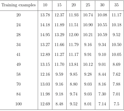
We test our method in the regression setting using the Parkinson’s disease telemonitoring dataset, which is composed of a range of biomedical voice measurements using a telemonitoring device from 42 people with early-stage Parkinson’s. The recordings were automatically captured in the patients’ homes. The aim is to predict the clinician’s Parkinson’s disease symptom score for each recording on the unified Parkinson’s disease rating scale (UPDRS) [47]. Thus we are in a regression setting, and employ the ϵ-insensitive loss from support vector regression. All kernels are taken to be Gaussian, and the random Fourier features speedup is used.

(43)

Table 2.1: RMSE of Marginal Transfer Learning on Parkinson’s Disease Dataset Training examples 10 15 20 25 30 35 20 13.78 12.37 11.93 10.74 10.08 11.17 24 14.18 11.89 11.51 10.90 10.55 10.18 28 14.95 13.29 12.00 10.21 10.59 9.52 34 13.27 11.66 11.79 9.16 9.34 10.50 41 12.89 11.27 11.17 9.91 9.10 10.05 49 13.15 11.70 13.81 10.12 9.01 8.69 58 12.16 9.59 9.85 9.28 8.44 7.62 70 13.03 9.16 8.80 9.03 8.16 7.88 84 11.98 9.18 9.74 9.03 7.30 7.01 100 12.69 8.48 9.52 8.01 7.14 7.5

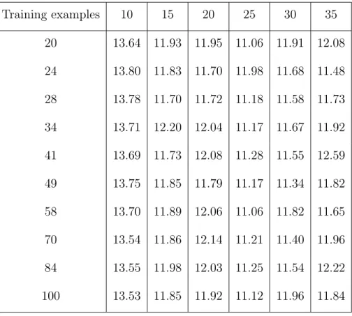
vary the number of training usersN from 10 to 35 in steps of 5, and we also vary the number of training examplesn per user from 20 to 100. We repeat this process several times to get the average errors which are shown in Fig 2.1 and Tables 2.1 and 2.2. The transfer learning method clearly outperforms pooling, especially as N andn increase.

II.6.3

Satellite Classification

Microsatellites are increasingly deployed in space missions for a variety of scientific and tech-nological purposes. Because of randomness in the launch process, the orbit of a microsatellite is random, and must be determined after the launch. One recently proposed approach is to estimate the orbit of a satellite based on radiofrequency (RF) signals as measured in a ground sensor network. However, microsatellites are often launched in bunches, and for this approach to be successful, it is necessary to associate each RF measurement vector with a particular

(44)

Table 2.2: RMSE of Pooling on Parkinson’s Disease Dataset Training examples 10 15 20 25 30 35 20 13.64 11.93 11.95 11.06 11.91 12.08 24 13.80 11.83 11.70 11.98 11.68 11.48 28 13.78 11.70 11.72 11.18 11.58 11.73 34 13.71 12.20 12.04 11.17 11.67 11.92 41 13.69 11.73 12.08 11.28 11.55 12.59 49 13.75 11.85 11.79 11.17 11.34 11.82 58 13.70 11.89 12.06 11.06 11.82 11.65 70 13.54 11.86 12.14 11.21 11.40 11.96 84 13.55 11.98 12.03 11.25 11.54 12.22 100 13.53 11.85 11.92 11.12 11.96 11.84

satellite. Furthermore, the ground antennae are not able to decode unique identifier signals transmitted by the microsatellites, because (a) of constraints on the satellite/ground anten-nae links, including transmission power, atmospheric attenuation, scattering, and thermal noise, and (b) ground antennae must have low gain and low directional specificity owing to uncertainty in satellite position and dynamics. To address this problem, recent work has proposed to apply our marginal transfer learning methodology [48].

As a concrete instance of this problem, suppose two microsatellites are launched together. Each launch is a random phenomenon and may be viewed as a task in our framework. For each launch i, training data (X_ij,Y_ij), j = 1, . . . ,n_i, are generated using a highly realistic

simulation model, whereX_ij is a feature vector of RF measurements across a particular sensor network and at a particular time, and Yij is a binary label identifying which of the two

(45)

Figure 2.1: Parkinson’s disease telemonitoring dataset

unlabeled measurementsXT_j from a new launch with high accuracy. Given these labels, orbits can subsequently be estimated using the observed RF measurements. We thank Srinagesh Sharma and James Cutler for providing us with their simulated data, and refer the reader to their paper for more details on the application [48].

To demonstrate this idea, we analyzed the data from [48] forT =50 launches, viewing 40 as

training data and 10 as testing. We use Gaussian kernels and the RFF kernel approximation technique to speed up the algorithm. Results are shown in Fig 2.2. As expected, the error for the proposed method is much lower than for pooling.

II.6.4

Flow Cytometry Experiments

We demonstrate the proposed methodology for the flow cytometry auto-gating problem, described in Sec. II.2. The pooling approach has been previously investigated in this context

(46)

Table 2.3: Average Classification Error of Marginal Transfer Learning on Satellite Dataset Training examples 10 20 30 40 5 8.62 7.61 8.25 7.17 15 6.21 5.90 5.85 5.43 30 6.61 5.33 5.37 5.35 45 5.61 5.19 4.71 4.70

all training data 5.16 4.72 3.69 3.87

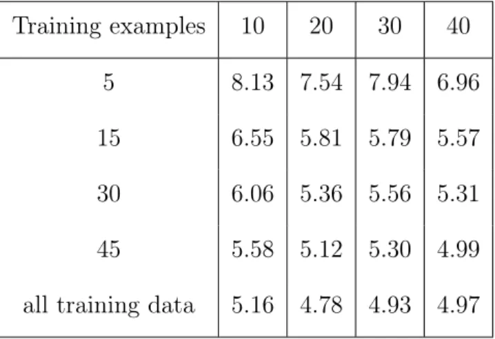
Table 2.4: Average Classification Error of Pooling on Satellite Dataset Training examples 10 20 30 40

5 8.13 7.54 7.94 6.96

15 6.55 5.81 5.79 5.57

30 6.06 5.36 5.56 5.31

45 5.58 5.12 5.30 4.99

(47)

Figure 2.2: Satellite dataset

by [49]. We used a dataset that is a part of FlowCAP Challenges where the ground truth labels have been supplied by human experts [50]. We used the so-called “Normal Donors" dataset. The dataset contains 8 different classes and 30 subjects. Only two classes (0 and 2) have consistent class ratios, so we have restricted our attention to these two.

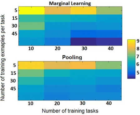
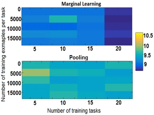
The corresponding flow cytometry data sets have sample sizes ranging from 18,641 to 59,411, and the proportion of class 0 in each data set ranges from 25.59 to 38.44%. We randomly selected 10 tasks as test tasks and used exactly the same tasks over all experiments. We varied the number of tasks in the training data from 5 to 20 with an additive step size of 5, and the number of training examples per task from 32 to 16384 with a multiplicative step size of 2. We repeated this process 10 times to get the average errors which are shown in Fig. 2.3 and Tables2.5 and 2.6. The kernelkP was Gaussian, and the other two were linear. The

Nyström approximation was used to achieve an efficient implementation.

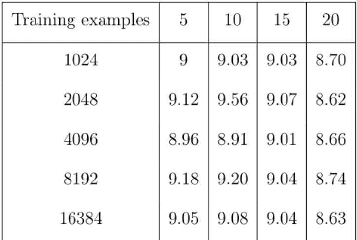
For nearly all settings the proposed method has a smaller error rate than the baseline. Furthermore, for the marginal transfer learning method, when one fixes the number of training

(48)

Table 2.5: Average Classification Error of Marginal Transfer Learning on Flow Cytometry Dataset Training examples 5 10 15 20 1024 9 9.03 9.03 8.70 2048 9.12 9.56 9.07 8.62 4096 8.96 8.91 9.01 8.66 8192 9.18 9.20 9.04 8.74 16384 9.05 9.08 9.04 8.63

Table 2.6: Average Classification Error of Pooling on Flow Cytometry Dataset Training examples 5 10 15 20 1024 9.41 9.48 9.32 9.52 2048 9.92 9.57 9.45 9.54 4096 9.72 9.56 9.36 9.40 8192 9.43 9.53 9.38 9.50 16384 9.42 9.56 9.40 9.33

(49)

Figure 2.3: Classification error rates for baseline and proposed method for different experi-mental settings, i.e., number of examples per task and number of tasks.

(50)

II.7

Multiclass Domain Generalization

In this chapter, we have reviewed kernel based approach to address domain generalization [32] which addresses binary classification and regression. In this section, we extend the generalization error analysis to multiclass setting ( |Y | =c ) and give supporting experimental results. While several aspects of the original analysis in [32] carry over to the multiclass case, others do not. In particular, we use an extension of the contraction lemma for Rademacher complexity of Lipschitz loss classes to prove the generalization error bound [51].

We modify our objective function for multiclass classification compared to Eqn. 2.5. We will find a decision function f ∈ H_¯c

k := Hk¯ × · · · Hk¯ (c times) and has components

д_l ∈ H_k¯,l =1,2, ...c, i.e., f =       д1 д2 · · · дc       . Define ˆ f_λ =arg min f∈H_¯c k 1 N N X i=1 1 ni ni X j=1 `(f(_X˜_ij_),_Y_ij₎₊_λr₍_f_), _(2.20)

as the empirical estimate of the optimal decision function. Define the regularizer r(f) as r(f) := kfk2_Hc ¯ k := c X m=1 kдmk_H2 ¯ k.

II.7.1

Generalization Error Analysis

We make the following assumptions to analyze the generalization error. For any kernelk, ϕ_k(x) := k(·,x) ∈ H_k denotes the canonical feature map, B_k(R) refers to the closed ball of radiusR inH_k and B_kc(R) :=

c

Y

m=1

B_k(R) refers to the product space ofc closed balls.

A I The loss function` :Rc × Y →R is bounded by B`, and isL`-Lipschitz in the first variable: For ally, |`(T1,y)−`(T2,y)| ≤L` kT1−T2k2 forT1,T2 ∈Rc.

(51)

A II Kernelskx,kx0,kP are bounded by B2_k,B_k20,B_k2

P respectively. A III The canonical feature mapϕ_k_P : H_k0

x → HkP is α-Hölder continuous, i.e., ∀a,b ∈ B_k0

x(Bk0) :

kϕ_k_P(a)−ϕ_k_P(b)k₂ ≤ L_k_Pka−bk₂α.

The above assumptions are similar to those presented in [52] translated to multiclass data. Condition A III holds with α = 1 whenkP is the Gaussian-like kernel on H_k0

x. Using the stated assumptions, we shall now develop generalization error bounds for multiclass DG. To generalize the analysis, an extension of Talagrand’s lemma for bounding the Rademacher complexity is needed. Such an extension was provided by [53, 51] and [54].

Lemma 2. (Vector Valued Talagrand’s Contraction Lemma) [51] Let F be a class

of functions from X →Rc. Let {µi}Ni=1 and {σij}

N,c

i=1,j=1 be two sets of independent Rademacher

random variables. If φ:Rc →R is L-Lipschitz under k·k_p where p ≥ 2, then

Eµ[ sup f∈F N X i=1 µiφ(f(xi))]≤ √ 2LEσ[ sup f∈F N X i=1 c X j=1 σijдj(xi)].

For simplicity’s sake, we assume thatni =n to state the generalization error bound.

Theorem 4. (Estimation error control) Assuming that conditionsA I-A III hold then for any R > 0, with probability at least 1−δ:

sup f∈Bc_¯ k(R) |_Dε(f)−ε(f)| ≤L`L_k_PRB_kc(B_k0)α s 2 log2_δN n + r 1 n + 4 log 2_δN 3n α + 8 √ 2RL`B_kB_k_Pc √ N +B` r log 8δ−1 2N

(52)

Proof Sketch Let E(f) = |ε_D(f)−ε(f)|. sup f∈Bc_¯ k(R) E(f) ≤ sup f∈B_¯c k(R) Dε(f)− 1 Nn N X i=1 n X j=1 `(f(_X˜_ij_),_Y_ij₎ + sup f∈Bc_¯ k(R) 1 Nn N X i=1 n X j=1 `(f(_X˜_ij_),_Y_ij₎₋_ε₍_f₎ = (I)+(II)

Term (I) is bounded by application of Lipschitz continuity of `, union bounds for tasks and classes over f and through Hölder continuity in assumption A III. Bounding the term (II) is similar to bounding term (II) in Theorem 5 in [52] with modifications for multi-class loss. In addition, the modified Talagrand’s lemma 2is applied to bound the Rademacher complexity [51].

II.7.2

Experimental Results

We test the proposed algorithm on 4 multiclass datasets and compare it with pooling, where data from all the tasks are pooled together to learn one single classifier. Datasets description are given below and a summary is in Table 2.7.

Dataset Training Tasks Test Tasks Examples Per Task Classes

Synthetic 80 20 100 10

Satellite 400 100 77-165 3

HAR 20 10 300 6

MNIST-MOD 80 20 100 10

Table 2.7: Summary of Multiclass Datasets for Domain Generalization

Kernel Methods for Learning with Limited Labeled Data