Temporal causal discovery and structure learning with attention based convolutional neural networks

(1)

Structure Learning with

Attention-Based Convolutional

Neural Networks

Master’s Thesis by

Meike Nauta

August 2018

Graduation Committee Dr. Christin Seifert Dr.ir. Maurice van Keulen Dr. Doina Bucur

(2)

(3)

Preface

This graduation project was an unpredictable but exciting journey that resulted in two di↵erent research projects, both on the topic ofcausal discovery and structure learning from observational data. This thesis presents the results of both projects to obtain the Master’s degree in Computer Science.

My first research project resulted in a paper named ‘LIFT: Learning Fault Trees from Observational Data’, that got accepted at the 15th _{International Conference on Quantitative Evaluation of SysTems}1

(QEST), that will be held from September 4-8 2018 in Beijing. This paper can be found on page 51 of this thesis. My main contribution however is the report of my second research project, called ‘Temporal Causal Discovery and Structure Learning with Attention-Based Convolutional Neural Networks’, which starts on page 1 of this thesis. In the following paragraphs, I will give a chronological overview of my graduation process that explains how I ended up with two di↵erent research projects.

My first research project started as part of the course ‘Research Topics’, which is intended to serve as a preliminary investigation for the final graduation project. I decided to join SEQUOIA2_{, a project funded by}

the Dutch STW that studies smart maintenance optimization for railroads by deploying machine learning techniques as well as fault tree analysis. A fault tree graphically models probabilistic causal chains of events that end in a global system failure. Since constructing a fault tree was largely a manual process, I chose to study the possibility to machine-learn a fault tree from observational data.

Since the decision tree is a tree formalism that is commonly machine-learnt from data, decision tree learning algorithms appeared to be a natural starting point for the design of a fault tree learning algorithm. However, I soon found out that decision trees model only correlations which would not provide root causes for faults. Since a fault tree needs to model causal relationships, I got into the topic of Causal Discovery that aims to discover causal relationships from observational data. At the end of the course, I had designed and implemented a causal discovery algorithm that could successfully learn a static fault tree. In my paper I not only present this algorithm, but I also introduce formal definitions for all elements in a fault tree.

Together with my supervisor dr. Doina Bucur and SEQUOIA project leader prof.dr. Mari¨elle Stoelinga, we decided that is was worthwhile to improve (and shorten) the paper such that it could be submitted to a conference. Since I already finished the Research Topics course, I spent the first 180 hours (±6 ECTS) of my final graduation project (credited for 30 ECTS in total) improving both the paper and the algorithm. In collaboration with Doina that wrote the main part of the related work section, and with the feedback of Mari¨elle, the paper got accepted at the International Conference on Quantitative Evaluation of SysTems (QEST).

After finishing this paper, I wanted to stay in the causal discovery domain but switched from learning fault trees to learning more generic causal graphs. Furthermore, whereas my fault tree algorithm was mainly based on statistics, I decided to change my scope to deep learning. Neural networks and their state-of-the-art performance in many classification and prediction tasks sparked my interests. Since most existing causal discovery methods use statistical measures, I had to be creative on how to apply deep learning for causal discovery. I very much enjoyed the design part of my project where I had to think out-of-the-box. I also learnt all kinds of deep learning techniques and causality jargon that I didn’t know about before.

Thanks to the critical yet valuable feedback of Doina Bucur, Christin Seifert, Maurice van Keulen and Yannick Donners, I have written a report that presents a deep learning framework based on attention-based convolutional neural networks that can successfully construct a temporal causal graph by discovering causal relationships in time series data. I am looking forward to continuing the research on this topic during my upcoming PhD at the University of Twente.

-Meike Nauta August 2018

1_{http://www.qest.org/qest2018/}

(4)

(5)

Contents of this Master’s Thesis

Temporal Causal Discovery and Structure Learning

with Attention-based Convolutional Neural Networks 1

(6)

(7)

Attention-Based Convolutional Neural Networks

Meike Nauta,

[email protected]

Abstract

We present the Temporal Causal Discovery Framework (TCDF), a deep learning framework that learns a causal graph structure by discovering causal relationships in observational time series data. TCDF uses attention-based convolutional neural networks to detect correlations between time series and subsequently performs a novel validation step to distinguish causality from correlation. By interpreting the internal pa-rameters of the convolutional networks, TCDF can also discover the time delay between a cause and the occurrence of its e↵ect. Our framework can learn both cyclic and acyclic causal graphs, which can include confounders and instantaneous e↵ects. The graph reduction step in TCDF removes indirect causal relation-ships to improve readability of the constructed graph. Using the representational power of deep learning, TCDF removes idealized assumptions upon the data that existing, usually statistical, causal discovery meth-ods make. Experiments on actual and simulated time series data show state-of-the-art performance of TCDF on discovering causal relationships in continuous, noisy and (non-)stationary time series data. Furthermore, we show that TCDF can circumstantially discover the presence of hidden confounders. Our broadly appli-cable framework can be used to gain novel insights into the causal dependencies in a complex system, which is important for interpretation, explanation, prediction, control and policy making.

(8)

Summary of Notation

Notation Meaning

X Dataset containingN time series all having the same lengthT, withN 2 andT 2.

Xi Theith row in datasetXcorresponding to one time series ofT time steps, with 0< iN. ˆ

Xi Predicted time series forXi.

X i All time series inXexceptXi. Xt

i Value of time seriesXi at time stept, with 0< tT. ˆ

Xt

i Predicted value forXit.

Ni Attention-based Dilated Depthwise Separable Temporal Convolutional Network (AD-DSTCN) that receivesXas input and outputs ˆXi.

G Temporal causal graph with a set of vertices and edges (V, E), denoting the causal relation-ships between time series inXand their delays.

G Complement of_G.

vi Vertex inV representing time seriesXi. ei,j Directed edge inEfrom vi tovj. E(_G) Set of edges in_G.

d(ei,j) Delay corresponding to edgeei,j denoting the number of time steps between the occurrence of causeXi and the occurrence of e↵ectXj.

s(ei,j) Causal strength score of causeXi on e↵ectXj. p=hvi, ..., vji Path from vertexvi to vertexvj.

|p| Length of a pathp=hvi, ..., vji, defined by the number of edges between vi andvj. d(p) Delay of a pathp=hvi, ..., vji, defined as the sum of delays of all edges inp.

GG Temporal causal graph denoting the ground truth causal relationships and their delays.

GF Temporal causal graph denoting the full ground truth causal relationships and their delays,

which contains an edgeei,j for each directed path fromvi tovj in_GG. GL Temporal causal graph that is learnt by a causal discovery method.

K Kernel size of an AD-DSTCN.

L Number of hidden layers in an AD-DSTCN. R Receptive field of a Convolutional Neural Network.

c Dilation coefficient.

f Dilation factor (i.e. step size), which equalscl _{for layer}_l. Learning rate of a neural network.

ai Attention vectorai= [a1,i, a2,i, ..., ai,i, ..., aN,i].

ai,j Attention score denoting how much_Nj attends to input time seriesXi. Wi The kernel weights ofNi.

⌧i Threshold to select the attention scores inai for causal validation.

hi Attention vectorai to which our HardSoftmax function is applied. hi,j Attention scoreai,j to which our HardSoftmax function is applied.

G List of gaps [g0, ..., gN 1] denoting the gaps between an ordered list of attention scores. gi Gap at positioniin G, denoting the value di↵erence between two attention scores. ↵i Learnable parameter used in the PReLU activation function in networkNi. F(x) Function applied by a convolutional layer to transform inputxto_F(x).

o Output of a convolutional layer after the activation function is applied.

Pi Set of potential causes for time seriesXi.

Ci Set of true causes for time seriesXi.

L Loss of a network, i.e. the error betweenXi and ˆXi.

LG Loss of a network when the real input distribution for CQII is used.

LI Loss of a network when the intervened distribution for CQII is used.

✏d(ei,j) The error of an incorrectly learnt delay, calculated as the distance from the ground truth delay to the learnt delay relative to the receptive field.

µ✏ Average error of all incorrectly learnt delays.

TP, FP Set of True Positives, resp. False Positives.

(10)

1 Introduction

What makes a stock’s price increase? What influences the water level of a river? Although machine learning has been successfully applied to predict these variables, most machine learning models cannot answer those questions. Existing machine learning models make predictions on the basis of correlations alone, but corre-lation does not imply causation [Kleinberg, 2015]. Measures of correcorre-lation aresymmetrical, since correlation only tells us that there exists a relation between variables. In contrast, causation is usuallyasymmetricaland therefore tells us the directionality of a relation between variables. For example, since height is correlated with age, age is also correlated with height. Only a causality measure can conclude if either age causally influences height, or that height has a causal influence on age. It could also be that, although height and age are correlated, there is no causal relationship between these variables. Correlation which is not causation often arises if two variables have a common cause, or if there is a spurious correlation such that the values of two unrelated variables are coincidentally statistically correlated.

Predictive models, e.g. decision trees and neural networks, do not make a distinction between correlation and causation and only learn correlations to increase their prediction accuracy [Nauta et al., 2018]. The relationships learnt by the model may be unstable if they are not causal, such that the model might stop working in the future. This will lead to wrong predictions, which is undesired if these predictions are used for decision making. If a model would learncausal relationships, we can make more robust predictions. In addition to making forecasts, the goal in many sciences is often to understand the mechanisms by which variables come to take on the values they have, and to predict what the values of those variables would be if the naturally occurring mechanisms were subject to outside manipulations [Spirtes, 2010]. Those mechanisms can be understood by discovering causal associations that explain the relationship between and occurrence of events. Knowledge of the underlying causes allows us to develop e↵ective policies to prevent or produce a particular outcome [Kleinberg, 2013].

The traditional way to discover causal relations is to manipulate the value of a variable by using in-terventions or real-life experiments. In an experimental setting, all other influencing factors of the target variable can be held fixed, such that it can be tested if a manipulation of a potential cause changes the target variable. However, such experiments and interventions are often costly, too time-consuming, unethical or even impossible to carry out. With the current advances in sensoring and Internet of Things, the amount of observational data grows extensively, allowing us to reveal (hypothetical) causal information by analysing this observational data, known as causal discovery [Zhang et al., 2017]. Causal discovery aims to help in interpreting data and formulating and testing hypotheses, which can be used to prioritize experiments and to build and improve theories or simulation models. Furthermore, causal discovery from observational data can be used to ensure the validity of experimental results that are often collected in restricted laboratory settings.

In this report, we focus on causal discovery from time series data, as the notion of time facilitates the discovery of the directionality of a causal relationship. After all, a cause generally happens before the e↵ect. Many algorithms have been developed in the last years to discover causal relationships from multivariate tem-poral observational data, particularly in the area of graphical causal modeling [Singh et al., 2018]. However, these usually statistical measures tend to rely on idealized assumptions that rarely hold in practice. Exist-ing approaches assume that the time series data is linear, stationary or without noise [Runge et al., 2017], [Huang and Kleinberg, 2015]. Furthermore, many methods assume that the underlying causal structure has no (hidden) common causes, is acyclic or does not have instantaneous e↵ects [Budhathoki and Vreeken, 2018], [Entner and Hoyer, 2010]. Furthermore, existing methods are only designed to discover causal associations, and they cannot be used to predict a variable’s value based on these discovered causal variables.

(11)

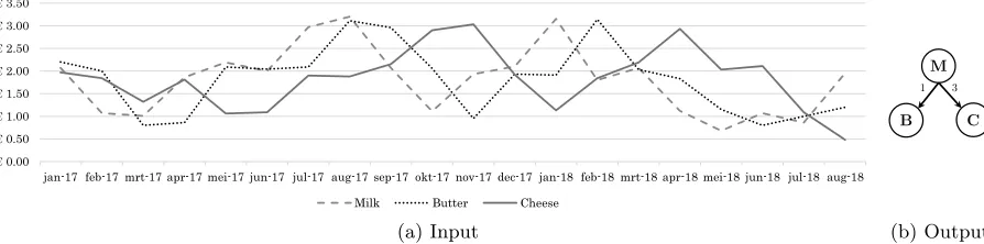
€ 0.00 € 0.50

€ 1.00 € 1.50 € 2.00 € 2.50 € 3.00 € 3.50

jan-17 feb-17 mrt-17 apr-17 mei-17 jun-17 jul-17 aug-17 sep-17 okt-17 nov-17 dec-17 jan-18 feb-18 mrt-18 apr-18 mei-18 jun-18 jul-18 aug-18

Milk Butter Cheese

(a) Input

B C

M

1 3

[image:11.612.82.529.78.189.2]

(b) Output

Figure 1: The plot (left) shows a fictive history of the prices of milk, butter and cheese. The data suggests that the price of milk causes the price of butter (with a delay of 1 month) and the price of cheese (with a delay of 3 months). Our framework receives the dairy prices as input and discovers the causal relationships and their delays to construct a temporal causal graph (right) showing the causal relationships and their delays between the prices of milk (M), butter (B) and cheese (C).

More specifically, in this report we present the Temporal Causal Discovery Framework (TCDF) that uses deep learning to:

1. Discovercausal relationships in time series data,

2. Discover thetime delaybetween cause and e↵ect of each causal relationship,

3. Learn atemporal causal graphbased on the discovered causal relationships with delays.

Our ambition is to provide a unified approach that exploits the representational power of deep learning and does not require any strong assumption on the data or underlying causal structure, in contrast to existing approaches.

For example, given a history of the prices of milk, butter and cheese, our framework could detect the causal relationships between these dairy products. Since milk is an ingredient of butter and cheese, the data should suggest that the price of milk causes the price of butter and that the price of milk causes the price of cheese. Furthermore, a change in the price of milk will probably be reflected in the price of butter resp. cheese with a certain delay. Figure 1 (left) shows a simple example containing fictive prices of milk, butter and cheese. It can be seen that the data suggests that the price of milk causes both the price of butter (with a delay of 1 month) and the price of cheese (with a delay of 3 months). Based on a dataset containing dairy prices, our framework can discover these causal relationships and their delays and can then visualize its findings in a temporal causal graph as shown in Figure 1 (right).

Thus, we require a dataset X containing N time series of the same length. These time series can be anything, from stock prices and weather data to water levels and heart rates. The goal is to discover the causal relationships between allN time series inX, including the delay between cause and e↵ect, and model this in a temporal causal graph.

Our framework, called Temporal Causal Discovery Framework (TCDF), consists of N convolutional neural networks, where each network receives allN observed time series as input. One network is trained to predict one time series. Thus, the goal of thejth _network_N

j is to predict each time step of its target time series Xj 2Xbased on past values. While a network performs supervised prediction, it trains its internal parameters using backpropagation.

(12)

After training the attention-based convolutional networks, TCDF distinguishes causation from correlation by applying a causal validation step. In this validation step, we intervene on a correlated time series to test if it is causally related with a predicted target time series. Each discovered time series that proves to be causal is included in a temporal causal graph that graphically shows the causal relationships between all time series.

In addition, we present a novel method to extract the learnt time delay between cause and e↵ect of each relationship from a network by interpreting the network’s internal parameters. TCDF then constructs a temporal causal graph in which both the discovered causal relationships and the discovered delays are included.

(13)

2 Background

This section provides background information on temporal causal discovery (Section 2.1), gives a global overview on how deep learning can be used for temporal causal discovery (Section 2.2) and discusses the most important challenges faced by causal structure learning methods (Section 2.3).

2.1 Temporal Causal Discovery

Causality has been an important concept for decades, as it is important for interpretation, explanation, prediction, control and policy making. Although the notion of causality has shown to be evasive when trying to formalize, we assume that a causal relationship should comply with two aspects [Eichler, 2012]:

1)Temporal precedence: the cause precedes its e↵ect,

2)Physical influence: manipulation of the cause changes its e↵ect.

The first assumption can only be validated when the time steps of all time series in the dataset are physically aligned (i.e. time steptfor one time series corresponds in the real world to time steptfor another time series). Using temporal data with the temporal precedence assumption also allows fordelay discovery, meaning that a model does not only detect the existence of a causal relationship but also the time delay between cause and e↵ect.

The second aspect is usually defined in terms of interventions. Since a cause is a way of bringing about an e↵ect, it can be understood in terms of how the probability or value of the e↵ect changes when manipulating the cause. More specifically, an observed time series Xi is a cause of another observed time series Xj if there exists an intervention onXi such that if all other time seriesX i 2Xare held fixed,Xi and Xj are associated [Woodward, 2005]. However, such controlled experiments in which other time series are held fixed may not be feasible in for example stock markets and many other time series applications. In those cases, researchers may be reluctant to test for physical influence. Another possibility, which is applied by TCDF, is to intervene onXi while assuming that all other time series X i2Xbehave as usual.

2.2 Deep Learning for Temporal Causal Discovery

The following paragraphs present some background information on the main concepts of our Temporal Causal Discovery Framework: Convolutional Neural Networks, Attention Mechanisms and the Causal Quantitative Input Influence.

Convolutional Neural Networks for Time Series Prediction A Convolutional Neural Network is a type of feed-forward neural network, consisting of a sequence of convolutional layers. A convolutional layer of a CNN limits the number of connections to only some of the input neurons by sliding akernel (a weight matrix) over the input and at each time step it computes the dot product between the input and the kernel. The kernel will then learn specific repeating patterns in the input series to forecast future values of the target time series. Intuitively, these learnt patterns denote correlations (and possibly causal relations) between the input series and the target output series which is important for causal discovery.

Until recently, Recurrent Neural Networks (RNNs), and in particular the Long-Short Term Memory unit (LSTM), were regarded as the default starting point to solve sequence learning. Because RNNs propagate forward a hidden state, they are theoretically capable of having infinite memory [Bai et al., 2018]. However, long-term information has to sequentially travel through all cells before getting to the present processing cell, causing the well-knownvanishing gradients problem [Bengio et al., 1994], [Glorot and Bengio, 2010]. Other issues with RNNs are the high memory usage to store partial results and the impossibility of parallelism which makes them hard to scale and not hardware friendly [Bai et al., 2018].

(14)

causal constraint that there can be no information ‘leakage’ from future to past. Furthermore, observational time series data usually contains only one repetition of the time series instead of observing a sequence several times. Convolutional architectures for time series are still scarce but recently successfully applied to finan-cial time series. [Borovykh et al., 2017] created a deep convolutional model for noisy finanfinan-cial time series forecasting and [Binkowski et al., 2017] presented a deep convolutional network for predicting multivariate asynchronous time series.

Attention Mechanism Recently, there has been a surge of work inexplainingdeep neural networks. One approach is to create an explanation-producing system that is designed to simplify the representation of its own behavior [Gilpin et al., 2018]. One successful explanation-producing method is the so-called attention mechanism. An attention mechanism (or ‘attention’ in short) equips a neural network with the ability to focus on a subset of its inputs. The concept of ‘attention’ has a long history in classical computer vision, where an attention mechanism selects relevant parts of the image for object recognition in cluttered scenes [Walther et al., 2004]. Only recently attention has made its way into deep learning. The idea of today’s attention mechanism is to let the model learn what toattend to based on the input data and what is has learnt so far. Besides the increased accuracy by using attention, an important advantage is that it gives us the ability tointerpret and visualize where the model attends to. This allowance of interpretability is why we propose attention mechanisms as a way to discover correlations.

Causal Validation To distinguish causation from correlation, we apply a causal validation step in which we intervene on the correlated time series to test the Physical influence assumption mentioned in Section 2.1. Only the time series that satisfy this constraint are considered to be causal and are included in the temporal causal graph.

Since we only use observational data and will not physically intervene in a system to do experiments, we apply theCausal Quantitative Input Influence (CQII)measure of [Datta et al., 2016] to allow for causal reasoning. This measure models the di↵erence in the “quantity of interest” between the real input distribution and an intervened distribution for a specific “input variable of interest”. This hypothetical intervened distribution is constructed by retaining the marginal distribution over all other inputs and sampling the input of interest from its prior distribution. In this way, the influence of an input can be quantified by measuring the di↵erence between the quantity of interest of the real input distribution and the intervened distribution.

As an example, the authors consider the case where an automated system assists in hiring decisions for a moving company [Datta et al., 2016]. Suppose that the input features used by this classification system areWeight Lifting Ability andGender. These variables are positively correlated with each other and with the hiring decisions made. In this example, the “quantity of interest” is the fraction of positive classification for women. To test for the influence of gender on positive classification for women, CQII replaces every woman’s field for gender with a random value. This value replacement is the ‘intervention’ used to construct the intervened distribution. To check for a causal association, the classification outcome based on the real input distribution is compared with the classification outcome of the intervened distribution where each gender field has a random value. If the intervention leads to a significant change in the classification outcome, thenGender is causally associated with positive classification.

(15)

1 3

X1 X2 X3

4

(a)X1 directly causesX2 with a delay of 1 time step,

and indirectly causesX3 with a total delay of 1 + 3 = 4 time steps.

1 2

4

X2 X3

X1

(b) Feedback loop between

X1,X2 andX3 with a delay of 2, resp. 4 resp 1

time steps.

3 X1 X2

1

(c) Self-causation ofX1 that repeatedly, with an interval of 3 time steps, causesX2with a delay of 1

time step.

3 1 4

X2 X3

X1

(d)X1 is a confounder of X2 andX3with a delay of

[image:15.612.78.536.70.178.2]

1 resp. 4 time steps.

Figure 2: Temporal causal graphs showing causal relationships and their delays between cause and e↵ect.

2.3 Causal Structure Learning and its Challenges

Structure learning is a model selection problem in which one estimates a graph that summarizes the depen-dence structure in a given data set [Drton and Maathuis, 2017]. In addition to performing temporal causal discovery which lists the causal relationships between observed time series, TCDF will perform temporal causal structure learning in which the discovered causal relationships between time series are visualized by acausal graph. This provides an intuitive understanding of the interrelations among the time series.

The starting point for causal graphical modeling is usually a directed graph in which an edgeei,jpointing from vertex vi to vertex vj represents a causal relationship from causeXi to e↵ect Xj. The graphs learnt by non-temporal i.i.d. structure learning methods include a vertex for each variable in the used dataset. For the modeling of temporal structures, there are two visualizations methods, which we call local and global graphical methods.

Local temporal causal structure learning methods (e.g. [Peters et al., 2013], [Entner and Hoyer, 2010]) make an adaptation to the i.i.d. approach by replicating the set of variables by the number of time steps such that a vertex represents one time step in one time series Xi. When no instantaneous e↵ects are discovered, such learnt graphs will be acyclic by design. The lack of cycles follows from the temporal precedence assumption, such that an edge from an early time vertex cannot a↵ect the past and will therefore always point to a later time vertex.

On the other hand, global graphical methods (e.g. [Budhathoki and Vreeken, 2018], [Jiao et al., 2013]) show that time seriesXi causes time seriesXj without taking a specific time stept into account . In such a learnt graph, a vertex denotes a time series Xi instead of referring to a specific time step in Xi, which is comparable to a discovered graph by non-temporal i.i.d. structure learning methods in which a vertex corresponds to an i.i.d. variable. The acyclicity restriction does not apply here, since feedback loops and self-causation may be allowed. For better readability and the discovery of global causal relationships, our framework constructs a graph where a vertex denotes a time series.

More formaly, in the directed causal graph_G= (V, E), vertex vi₂V represents an observed time series

Xi and each directed edgeei,j 2E from vertexvi to vj denotes a causal relationship where time seriesXi causes an e↵ect in Xj. Furthermore, we denote byp=hvi, ..., vjia path inGfrom vito vj. The length of a path (counted as the number of edges) is denoted as|p|.

In ourtemporal causal graph, every edgeei,j is annotated with a numberd(ei,j), that denotes the time delay between the occurrence of causeXiand the occurrence of e↵ectXj. An example of a simple temporal causal graph is shown in Figure 2a. The sum of the delays of all edges in pathp is denoted asd(p). The goal of this study is not only to perform temporal causal discovery, but also to learn a temporal causal graph from observational time series data.

(16)

indirect causality [Papana et al., 2016], such that onlyek,j would be included in their graphG.

Secondly, it is relevant to correctly infer instantaneous causal e↵ects, where the delay between cause and e↵ect is 0 time steps. Neglecting instantaneous influences can lead to misleading interpretations of causal e↵ects [Hyv¨arinen et al., 2008]. In practice, instantaneous e↵ects mostly occur when cause and e↵ect refer to the same time step that cannot be causally ordered a priori because of a too coarse time scale.

Moreover, it is important that a causal structure learning method does not rely on the idealized assump-tion that a directed graph should be acyclic. Since real-life systems may exhibit repeated behavior, there can befeedback loops(Fig. 2b) orself-causation(Fig. 2c) [Kleinberg, 2013].

Lastly, the presence of aconfounder, a common cause of at least two variables, is a well-known challenge for structure learning methods (Fig. 2d). Although confounders are quite common in real-world situations, they complicate causal discovery since the confounder’s e↵ects are correlated with each other but they are not causally associated. Especially when the delays between the confounder and its e↵ects are not equal, one should be careful to not incorrectly include a causal relationship between the confounder’s e↵ects (the grey edge in Fig. 2d). Going back to the milk price example from the Introduction, a machine learning model might incorrectly learn that the price of butter causes the price of cheese, since the delay between milk price (X1) and butter price (X2) is lower than the delay between the milk price and cheese price (X3) because of the long storage period of cheese.

(17)

3 Related Work

Many di↵erent causal discovery algorithms have been developed to learn a causal graph from observational data. These algorithms are principally used to discover hypothetical causal relations between variables, in the context of other relevant or irrelevant variables. Most causal discovery methods construct a causal graph based on statistical tests. Pathways in the graph correspond to probabilistic dependence, and graphical non-adjacencies imply independence. These methods usually assume that the data satisfies the Causal Markov Condition, meaning that every variable in the dataset is independent of its non-e↵ects conditional on its direct causes [Malinsky and Danks, 2018].

Literature distinguishes two common approaches to efficiently discover a causal graph structure given non-temporal i.i.d. (independent and identically distributed) observational data: score-based methods and constraint-based methods [Malinsky and Danks, 2018]. Score-based methods iteratively optimize a causal structure by scoring a specific structure on the basis of some measure of model fit, and return the causal structure with the best score. In contrast, constraint-based methods rule out all causal structures that are incompatible with a foreknown list of invariance properties, and return the set of causal graphs that imply exactly the (conditional) independencies found in the data [Kalisch and B¨uhlmann, 2014].

Temporal data present a number of distinctive challenges and can require quite di↵erent causal search algorithms [Malinsky and Danks, 2018]. Since there is no sense of time or prediction in the usual i.i.d. setting, causality as defined by the i.i.d. approaches is not philosophically consistent with causality for time series, as temporal data should also comply with the ‘temporal precedence’ assumption [Quinn et al., 2011]. Furthermore, an important di↵erence is that in practice temporal observational data contains only one repetition of the time series instead of observing every variable several times [Peters et al., 2017].

For the scope of this chapter, we will introduce di↵erent categories for temporal causal discovery and give a selective overview of recent causal discovery algorithms for time series data in Section 3.1. We refer the reader to [Kalisch and B¨uhlmann, 2014] for an extensive review of non-temporal causal structure learning methods for non-temporal data. A more recent survey for non-temporal causal discovery techniques is [Singh et al., 2018] in which the authors present a comparative experimental benchmarking.

In Section 3.2, we propose the introduction of a new category for temporal causal discovery: Deep Learning. To the best of our knowledge, there does not yet exist a deep learning model for temporal causal discovery. However, we discuss some recent causal discovery methods for non-temporal observational data that use deep learning techniques.

3.1 Temporal Causal Discovery Methods

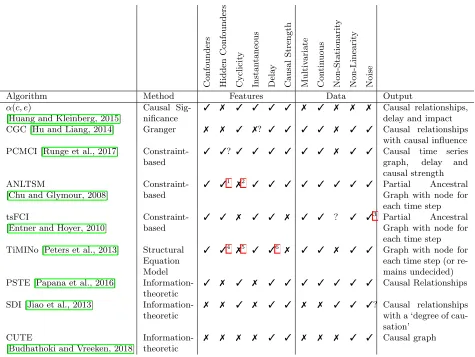
Table 1 shows recent temporal causal discovery models, categorised in five di↵erent approaches and assessed along various dimensions. Each approach is discussed in more detail in the paragraphs below Table 1. The table only reflects some of the most recent approaches for each type of model, since the amount of literature is very large.

Features The subcolumns in the ‘Features’ column in Table 1 denote if the algorithm can deal with confounders and cyclic graphs (i.e. feedback loops and self-causation), and if it can measure instantaneous e↵ects, delay between cause and e↵ect and the causal strength of a causal relationship. We consider causal strength as being some kind of quantitative measure that indicates how strongly one time series influences another.

(18)

C o n fo u n d ers H id d en C o n fo u n d ers Cyc lic it y Ins tan tane ous De la y C a u sa l S tre ng th M u lt iv a ri a te Co n tin u o u s N o n -S ta ti o n a ri ty N o n -L in ea ri ty Noise

Algorithm Method Features Data Output

↵(c, e)

[Huang and Kleinberg, 2015]

Causal Sig-nificance

3 7 3 3 3 3 7 3 7 7 7 Causal relationships,

delay and impact

CGC [Hu and Liang, 2014] Granger 7 7 3 7? 3 3 3 3 7 3 3 Causal relationships

with causal influence

PCMCI [Runge et al., 2017]

Constraint-based

3 3? 3 3 3 3 3 3 7 3 3 Causal time series

graph, delay and

causal strength ANLTSM

[Chu and Glymour, 2008]

Constraint-based

3 31 ₇2 ₃ ₃ ₃ ₃ ₃ ₃ ₃ ₃ _Partial _Ancestral

Graph with node for each time step tsFCI

[Entner and Hoyer, 2010]

Constraint-based

3 3 7 3 3 7 3 3 ? 3 33 _Partial _Ancestral

Graph with node for each time step

TiMINo [Peters et al., 2013] Structural

Equation Model

3 34 ₇5 ₃ ₃6 ₇ ₃ ₃ ₇ ₃ ₃ _{Graph with node for}

each time step (or re-mains undecided)

PSTE [Papana et al., 2016]

Information-theoretic

3 7 3 7 3 3 3 3 3 3 3 Causal Relationships

SDI [Jiao et al., 2013]

7 7 3 7 3 3 7 7 3 3 3? Causal relationships

with a ‘degree of cau-sation’

CUTE

[Budhathoki and Vreeken, 2018]

[image:18.612.72.547.67.424.2]

7 7 7 7 3 3 7 7 7 3 3 Causal graph

Table 1: Causal discovery methods for time series data, classified among various dimensions. A ‘?’ indicates that we are unsure.

Granger Causality(GC) [Granger, 1969] is one of the earliest methods developed to quantify the causal e↵ects among two time series (therefore called a ‘pairwise’ method). It is based on the common conception that a cause occurs prior to its e↵ect. More precisely, time series Xi Granger causes time series Xj if the future value of Xj (at time t+ 1) can be better predicted by using both the values of Xi and Xj up to time t than by using only the past values of Xj itself. However, in practice not all relevant variables may be observed or measured. This reveals an important shortcoming of GC; it cannot correctly deal with unobserved time series, including hidden confounders [Bahadori and Liu, 2013].

Furthermore, although GC is successfully applied across many domains, it only captures the linear interdependencies among time series. Various extensions have been made to nonlinear and higher-order causality, e.g. [Ancona et al., 2004], [Marinazzo et al., 2008] and [Luo et al., 2013]. A more recent extension that outperforms other Granger causality methods is based on conditional copula, that allows to dissociate the marginal distributions from their joint density distribution to focus only on statistical dependence between variables for uncovering the temporal causal graph [Hu and Liang, 2014].

1_{Requires hidden confounders to be instantaneous and linear.}

2_{The authors present another version of the model that allows feedback loops, but only in the absence of hidden confounders.} 3_{Assumes Gaussian noise.}

4_{TiMINo stays undecided by not inferring a causal relationship in case of a hidden confounder.} 5_{Cyclicity is theoretically shown, but the algorithm is only implemented to produce acyclic graphs.}

(19)

Constraint-based Time Series approachesare often adapted versions of non-temporal causal graph discovery algorithms for random variables. As an additional advantage, the temporal precedence constraint helps reduce the search space of the causal structure [Spirtes and Zhang, 2016]. The well-known causal discovery algorithms PC and FCI both have a time series version: PCMCI [Runge et al., 2017] and tsFCI [Entner and Hoyer, 2010].

The PC algorithm (named after its authors, Peter and Clark) [Spirtes et al., 2000] makes use of a clever series of tests to efficiently explore the whole space of DAGs (Directed Acyclic Graphs). FCI (Fast Causal Inference) [Spirtes et al., 2000] is a constraint-based algorithm that, contrary to PC, can deal with hidden confounders by using independence tests on the observed data. However, both algorithms produce an acyclic graph and therefore do not allow feedback loops. Besides, [Chu and Glymour, 2008] developed ANLTSM (Additive Non-linear Time Series Model) for causal discovery in both linear and non-linear time series data, that can also deal with hidden confounders. It uses statistical tests based on additive model regression.

Structural Equation Model approachesassume that the causal system can be represented by a Struc-tural Equation Model (SEM) that describes a variableXjas a function of other substantive variablesX jand a unique error term ✏X to account for additive noise such thatX :=f(X j,✏X) [Spirtes and Zhang, 2016]. It assumes that the set X j is jointly independent. SEM approaches are applied in the i.i.d. setting, but [Peters et al., 2013] presented TiMINo (Time Series Model with Independent Noise) for the case of stationary time series data. TiMINo associates the SEM with a directed graph that contains each time stepXt

i 2Xi as a node in the so-calledfull time graph. There is a directed edge fromXittoXjt,i6=j, if the coefficient of Xt

i is nonzero forXjt. The resultingsummary time graph contains all time series as vertices in which there is an edge fromXi toXj if there exists an edge fromXit k toXjtin the full time graph for somek.

Note, since TiMINo requires i ₆= j, that self-causation is not allowed. Furthermore, TiMINo remains undecided if the direct causes of Xi are not independent, instead of drawing possibly wrong conclusions. However, the main disadvantage is that TiMINo is not suitable for large datasets, since even smallest di↵erences between the true data and the model may lead to rejected independence tests. Furthermore, the authors state that the results from a high-dimensional dataset (more than ten time series) should be interpreted carefully.

There are also Information-theoretic approaches for temporal causal discovery such as (mutual) shifted directed information [Jiao et al., 2013] and transfer entropy [Papana et al., 2016]. Their main ad-vantage is that they are model free and make no assumption for the distribution of the data, while being able to detect both linear and non-linear dependencies [Papana et al., 2014]. The universal idea is thatXi is likely a cause ofXj,i6=j, ifXj can be better sequentially compressed given the past of bothXi andXj than given the past ofXj alone.

Compared to transfer entropy, directed information can be extended to more general systems, is not lim-ited to stationary Markov processes and is able to quantify the instantaneous causality [Liu and Aviyente, 2012]. To solve the problem of transfer entropy not being able to deal with non-stationary time series,

[Papana et al., 2016] introduced Partial Symbolic Transfer Entropy (PSTE). However, PSTE is not e↵ective when only linear causal relationships are present in the underlying causal system.

Besides, [Budhathoki and Vreeken, 2018] introduced CUTE (Causal Inference on Event Sequences) that is claimed to be more robust than transfer entropy, but can only handle discrete data.

(20)

3.2 Causal Discovery Methods based on Deep Learning

Existing temporal causal discovery methods, as discussed in the previous section, are mainly based on statistical measures. Deep Learning, the approach we propose, is not yet used for temporal causal discovery. The only study we found that compared deep learning with existing causality measures, was [Guo et al., 2018] that proposed an interpretable LSTM network to characterize variable importance. Using an attention mechanism, the important variables found by the LSTM showed to be highly in line with those determined by the Granger causality test [Granger, 1969]. This exhibits the prospect that deep learning methods are suitable for causal discovery.

(21)

4 Temporal Causal Discovery Framework

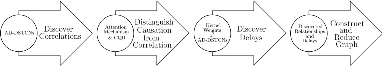
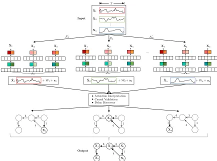
This chapter introduces and explains our Temporal Causal Discovery Framework (TCDF). Figure 3 gives a global overview of TCDF, showing that TCDF applies 4 steps to learn a Temporal Causal Graph from observational data: Correlation Discovery, Causal Discovery, Delay Discovery and Graph Construction.

Discover Correlations AD-DSTCNs

Distinguish Causation

from Correlation Attention

Mechanism & CQII

Discover Delays Kernel

Weights of AD-DSTCNs

Construct and Reduce

Graph Discovered

[image:21.612.116.497.150.219.2]

Relationships and Delays

Figure 3: Overview of our Temporal Causal Discovery Framework (TCDF). The arrows describe the steps taken by TCDF, while the circles describe what TCDF uses to perform the corresponding step.

More specifically, our Temporal Causal Discovery Framework (TCDF) consists ofNindependent attention-based convolutional neural networks, all having the same architecture but a di↵erent target time series. An overview of TCDF containing multiple networks is shown in Figure 4. This shows that the goal of the jth network_Nj is to predict itstarget time seriesXj by minimizing the lossLbetween the actual values ofXj and the predicted ˆXj. The input to network_Nj consists of aN⇥T dataset Xconsisting ofN equal-sized time series of lengthT. RowXj from the dataset corresponds to thetarget time series, while all other rows in the dataset,X j, are the so-calledexogenous time series.

When network Nj is trained to predictXj, the attention scoresaj of the attention mechanism explain where network Nj attends to when predicting Xj. Since the network uses the attended time series for prediction, the attended time series should contain information that is useful for prediction, implying that the attended time series are correlated with the predicted target time series Xj. TCDF therefore use the attention scores to discover which of the exogenous time series are correlated with the targetXj. By including the target time series in the input as well, the attention mechanism can also learn self-causation. We designed a specific architecture for these attention-based convolutional networks that allows TCDF to discover these correlations. We call our networks Attention-based Dilated Depthwise Separable Temporal Convolutional Networks (AD-DSTCNs). Based on the attention scores of AD-DSTCN_Nj, TCDF can discover which time series are correlated withXj.

The rest of this chapter is structured as follows: Section 4.1 describes the architecture of AD-DSTCNs and discusses in more detail how TCDF uses these to discover correlations in a dataset. Section 4.2 describes the second step of TCDF (shown in the middle of Figure 4) distinguishing causal relationships from all discovered correlations by interpreting the attention results and applying the Causal Quantitative Input Influence (CQII) to validate if a correlation is a causation. As a third step, TCDF discovers the time delay between the cause and e↵ect of each discovered causal relationship. For this delay discovery, TCDF uses the kernel weights_Wj of each AD-DSTCNNj, which will be discussed in more detail in Section 4.3. Lastly, TCDF merges the results of all networks to construct a Temporal Causal Graph that graphically shows the discovered causal relationships and their delays. For better readability, TCDF applies a graph reduction step that removes all discovered indirect causes. Section 4.4 describes the graph construction and reduction in more detail.

4.1 Correlation Discovery with AD-DSTCNs

(22)

Input

Output

T

... X1

X2

Xn

• • •

3

1 4 6

1 X2

1 1

6 3

4 X1

X1 X2 Xn

ˆ

X2 +W2+a2

X1 X2 Xn

ˆ

X1 +W1+a1

N2 N1

X1 X2 Xn

ˆ

Xn +Wn+an

1 1

6 3

4

1 1

6 3

4

Nn

Xn . . .

X1 Xi X2

Xn Xj

[image:22.612.104.538.205.527.2]

Attention Interpretation Causal Validation Delay Discovery

(23)

4.1.1 Temporal Convolutional Network

An important restriction for time series prediction is that a neural network may not access future values when predicting the current value of a time series. Therefore, we use the generic Temporal Convolutional Network (TCN) architecture of [Bai et al., 2018] as a basis for our network architecture. This convolutional architecture has configurable settings that can be used for univariate time series modeling. Having one time seriesX1 (which could be the price of milk for example) as input, TCN can predict a di↵erent target time series X2 (say, the price of cheese). TCN consists of a 1-dimensional (1D) Convolutional Neural Network architecture in which each layer has lengthT, whereT is the number of time steps of the input time series and the equally-sized target time series. TCN uses supervised learning by minimizing the loss _L between the actual values of targetX2 and the predicted ˆX2. A TCN predicts time step t of the target time series based on the past and current values of the input time series, i.e. from time step 1 up to and including time step t. Including the current value of the input time series enables the detection of instantaneous e↵ects. Since no future values are used for prediction, it satisfies the causal time constraint that future information cannot cause an e↵ect. Therefore, a TCN uses a so-calledcausal convolutionin which there is no information ‘leakage’ from future to past.

A TCN predicts each time step of the target time series X2 by sliding a kernel over inputX1 of which the input values are [X1

1, X12, ..., X1t, ..., X1T]. When predicting the value ofX2at time stept, denoted asX2t, the 1D kernel with a user-specified size Kcalculates the dot product between the learnt kernel weights W, and the current input value plus itsK 1 previous values, i.e. _W [X₁t K+1, X₁t K+2..., X₁t 1, Xt

1]. However, when the first value of X2, denoted asX21, has to be predicted, the input data only consists of X11 and past values are not available. This means that the kernel cannot fill its kernel size if K >1. Therefore, TCN appliesleft zero padding such that the kernel can access K 1 values that equal zero to replace the missing past values. For example, ifK= 4, the sliding kernel first sees [0,0,0, X1

1], followed by [0,0, X1

1, X12], [0, X11, X12, X13], etc. until [X1T 3, X T 2 1 , X

T 1 1 , X1T].

4.1.2 Discovering Self-causation

Whereas the authors of TCN assume that the input time series is di↵erent than the output time series, we propose to allow the input and output time series to be the same. Having the target time seriesXj as input data allows us to discover self-causation (i.e. the target time series causally influences itself, which enables the modeling of repeated behavior). However, in this case we have to slightly adapt the TCN architecture of [Bai et al., 2018], since we cannot include the current value of the target time series in the input. With an exogenous time series as input, the sliding kernel with size Kcan access [Xit K+1, Xit K+2..., Xit 1, Xit] withi6=j to predictXt

j for time stept. However, with the target time series as input, the kernel may only access thepastvalues of the target time seriesXj, i.e. excluding the current valueXjtsince that is the value to be predicted.

Therefore, we have to make sure that this current value cannot be seen by the kernel. A simple so-lution to this is to shift the target input data one time step forward with left zero padding such that the input target time series in the dataset equals [0, X1

j, Xj1, ..., X T 1

j ] and the kernel therefore can access [Xjt K, Xjt K+1..., Xjt 2, Xjt 1] to predictXjt.

4.1.3 Multivariate Causal Discovery

(24)

ˆ

X1

2 Xˆ22Xˆ23Xˆ42Xˆ52Xˆ62Xˆ27Xˆ28Xˆ29Xˆ210Xˆ112Xˆ212Xˆ213

X1

2X22X23X42X25X62X27X28X29X210X211X212X213

X1

nXn2Xn3Xn4Xn5Xn6Xn7Xn8X9nXn10Xn11Xn12Xn13

...

... X1

1X12X13X41X15X61X17X81X91X110X111X112X113

Input

Hidden

Output

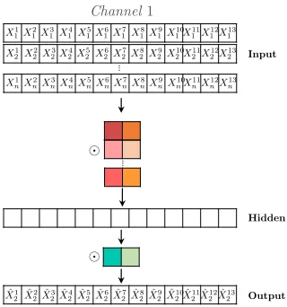
[image:24.612.238.398.69.240.2]

Channel1

Figure 5: A Multivariate Temporal Convolutional Network that predictsX2based on a 2D-input containing N time series with T = 13 time steps. The network has L= 1 hidden layer and 2 kernels with kernel size K = 2 (denoted by the colored blocks). The kernel in the first layer has a kernel height of N. The time series are element-wise multiplied with the kernel weights (denoted by ).

To allow for multivariate causal discovery, we therefore extend the univariate TCN architecture to a 1-dimensionalDepthwise Separable Temporal Convolutional Network(DSTCN) in which the input time series stay separated. A DSTCN consists of one channel for each input time series makingN channels in total. Thus, in network_Nj, channeljcorresponds to the target time seriesXj = [0, Xj1, Xj1, ..., XjT 1] and all other channels correspond to the exogenous time seriesXi6=j = [Xi1, Xi1, ..., X

T 1

i , XiT]. An overview of this architecture is shown in Figure 6. This overview includes the attention mechanism that will be discussed in Section 4.1.7.

A depthwise separable convolution consists of depthwise convolutions, where channels are kept separate by applying a di↵erent kernel to each input channel, followed by a 1_⇥1 pointwise convolution that merges together the resulting output channels [Chollet, 2017]. This is di↵erent than normal convolutional architec-tures that have just one kernel per layer. Because of the separate channels, the kernel weights relate to one specific time series which allows us to correctly interpret the relation between a specific input time series and the target time series, without any mixing of inputs. This shows to be useful for our delay discovery.

But, although a separate channel for each input time series is useful for correctly interpreting how one specific time series influences the target, it is not sufficient for accurate time series prediction. When predicting the target time seriesXj conditional on another time seriesXiwherei6=j, we should also include the past values of targetXj. More formally, we aim at maximizing the conditional likelihood:

P(Xj|Xi6=j) = T

Y

t=1

P(Xjt|Xi1, ..., Xit, Xj1, ..., Xjt 1). (1)

Adopting the idea from [Borovykh et al., 2017] for time series prediction, the conditioning on past values ofXj is done by element-wise addition of the target convolutional output from the first layer to the convo-lutional outputs from the first layer of the other channels. The element-wise addition is indicated by in Figure 6. With this addition, we ensure that each channel uses not only the past and current values of their input time series, but also the past values of the target time series.

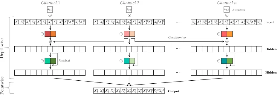
4.1.4 Activation Functions

(25)

ˆ

X1

2Xˆ22Xˆ32Xˆ24Xˆ25Xˆ62Xˆ27Xˆ82Xˆ29Xˆ210Xˆ211Xˆ122Xˆ213

a2,1

X1

2X22X23X24X25X62X27X82X92X210X112X122X213

a2,2

X1

nXn2Xn3X4nX5nXn6Xn7X8nXn9Xn10Xn11X12nX13n a2,n

De

pth

w

is

e

Po

in

tw

is

e

X1

1X12X31X14X15X16X71X81X19X101X111X112X113 ...

...

Input Attention

Hidden

Output Conditioning

Channel1 Channel2 Channeln

[image:25.612.75.540.71.230.2]

Residual

Figure 6: Attention-based Dilated Depthwise Separable Temporal Convolutional NetworkN2 to predict its target time series X2, having N channels withT = 13 time steps, L= 2 hidden layers and N⇥L kernels with kernel sizeK= 2 (denoted by the colored blocks). The attention scoresaare element-wise multiplied with the input time series, followed by an element-wise multiplication with the kernel. The output of the first convolution from target X2 is element-wise added to the other outputs before being inputted to the next convolutional layer. In the pointwise convolution, all output channels are combined to construct the prediction ˆX2.

forecasting of non-stationary, noisy financial time series [Borovykh et al., 2017], and has shown to improve model fitting with nearly zero extra computational cost and little overfitting risk compared to the traditional ReLU [He et al., 2015].

But, since we have a regression task, the network needs to be able to approximate any real value, without being changed by a non-linear activation function. Therefore, we use the common setup that applies a linear activation function in the last hidden layer7_{. Moreover, it has been shown that neural} networks that combine linear and nonlinear feature transformations are able to capture long-term temporal correlations [M¨uller et al., 2012].

4.1.5 Residual connections

An increasing number of hidden layers in a network usually results in a higher training error. This accuracy degradation, called thedegradation problem, is not caused by overfitting, but because standard backpropa-gation tends to become unable to find optimal weights in a deep network [He et al., 2016]. The proven way around this problem is to use residual connections. A convolution layer transforms its inputxto_F(x), after which an activation function is applied. With a residual connection, the inputxof the convolutional layer is added to_F(x) such that the outputo is:

o= PReLU(x+_F(x)) (2)

We add a residual connection in each channel after each convolution from the input to the convolution to the output, as shown in Figure 6. We only exclude the first layer since here already the target conditioning takes place.

(26)

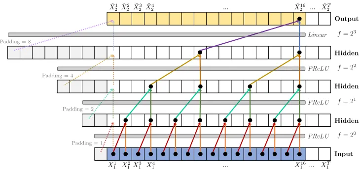
ˆ

X1

2 Xˆ22 Xˆ23Xˆ42 ... Xˆ162 ... Xˆ2T

Output

Hidden

Input

X1

1 X12X13 X14 ... X116... X1T

Padding = 8

Padding = 4

Padding = 2

Padding = 1

f= 23

f= 22

f= 21

f= 20 Linear

PReLU

[image:26.612.106.471.69.244.2]

PReLU

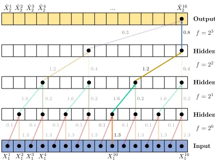
Figure 7: Channel 1 of a dilated DSTCN to predictX2, withL= 3 hidden layers, kernel sizeK= 2 (denoted by the arrows) and dilation coefficientc= 2, leading to a receptive fieldR= 16. A ReLU activation function is applied after each convolution. To predict the first values (shown by the dashed arrows), zero padding is added to the left side of the sequence. Weights are shared across layers, indicated by the identical colors.

4.1.6 Dilations

In a TCN with only one layer (i.e. no hidden layers), the receptive field (the number of time steps seen by the sliding kernel) is equal to the user-specified kernel sizeK. To successfully discover a causal relationship, the receptive field should be as least as large as the delay between cause and e↵ect. To increase the receptive field, one can increase the kernel size or add hidden layers to the network.

A 1D convolutional network has a receptive field that grows linearly in the number of layers, which is computationally expensive when a large receptive field is needed. More formally, the receptive fieldR of a 1D CNN is

RCN N = 1 + L

X

l=0

(k 1) (3)

where K is the user-specified kernel size and L the number of hidden layers. (L= 0 corresponds to a network without hidden layers, where one convolution in a channel maps an input time series to the output.) The well-known WaveNet architecture [Van Den Oord et al., 2016] therefore employed dilated convolu-tions. A dilated convolution is a convolution where a kernel is applied over an area larger than its size by skipping input values with a certain step sizef. This step sizef, calleddilation factor, increases exponen-tially depending on the chosen dilation coefficient c, such that f =cl _{for layer} _{l. An example of dilated} convolutions is shown in Figure 7.

With an exponentially increasing dilation factor f, a network with stacked dilated convolutions can operate on a coarser scale without loss of resolution or coverage. We therefore implement the dilated convolutions to create a Dilated DSTCN (D-DSTCN). The receptive field R of a kernel in a 1D Dilated DSTCN is:

RD DST CN = 1 + L

X

l=0

(k 1)_·cl (4)

(27)

4.1.7 Attention Mechanism

The D-DSTCN architecture as described in the previous paragraphs is suitable for time series prediction. However, we need to add a method to the network architecture that extracts explanations from the network, such that our framework TCDF can discover which time series are correlated with the predicted time series. We therefore add an explanation-producing method called ‘attention mechanism’ [Gilpin et al., 2018] to our network architecture. We call these attention-based networks ‘Attention-based Dilated Depthwise Separable Temporal Convolutional Networks’ (AD-DSTCNs).

An attention mechanism (or attention in short) equips a neural network with the ability to focus on a subset of its inputs. Prior work on attention in deep learning mostly addresses recurrent networks, but Face-book’s FairSeq [Gehring et al., 2017] for neural machine translation and the Attention Based Convolutional Neural Network (ABCNN) [Yin et al., 2016] for modelling sentence pairs have shown that attention is very e↵ective in CNNs as well. Besides the increased accuracy, attention allows us to interpret where the network attends to. Thus, after training a network on predicting the target time seriesXj, we can identify to which input time series networkNj attended to. These attended time series should be at least correlated with the predicted target time series and might have a causal influence on the target.

Typically, attention is implemented as a trainable 1 _⇥N-dimensional vector a that is element-wise multiplied with the N input time series or with the output of another neural network. Each value a ₂

a is called an attention score. In our framework, each network _Nj has its own attention vector aj = [a1,j, a2,j, ..., aj,j, ..., aN,j]. Attention score ai,j is multiplied with input time seriesXi in networkNj. This is indicated with at the top of Figure 6. Thus, attention score ai,j ₂aj shows how muchNj attends to input time series Xi for predicting targetXj. A high value for ai,j 2aj means thatXi is correlated with

Xj and might cause Xj. A low value for ai,j means that Xi is not correlated with Xj. Note that i =j is possible since we allow self-causation. The attention scores will be used after training of the networks to determine which time series are correlated with a target time series.

4.1.8 Correlation Discovery

Our framework has one AD-DSTCN for each time series Xj 2 X. All N AD-DSTCNs have the same architecture, but only their target time series is di↵erent. Network_Nj is trained to predict its target time seriesXj with backpropagation by minimizing the error between the actual values ofXj and the predicted values ˆXj. The number of training epochs, loss function and optimization algorithm can be selected by the user.

When the training of the network starts, all attention scores are initialized as 1 such thataj= [1,1, ...,1]. While the networks use back-propagation to predict their target time series, the network also changes its attention scores such that each score is either increased or decreased in every training epoch. This means that after some training epochs,aj2[ 1,1]N although the boundaries depend on the number of training epochs and the specified learning rate.

Literature distinguishes betweensoft attention whereaj2[0,1]N, andhardattention whereaj 2{0,1}N. Soft attention is usually realized by applying the Softmax function to the attention scores such that

PN

i=1ai,j = 1. A limitation of the Softmax transformation is that the resulting probability distribution always has full support, i.e. (ai,j)₆= 0 [Martins and Astudillo, 2016].

Intuitively, one would prefer hard attention for correlation discovery, since the network should make a binary decision: a time series is either correlated (and possibly causally related) or non-correlated. However, hard attention is non-di↵erentiable due to its discrete nature and therefore cannot be optimized through back-propagation [Shen et al., 2018]. We therefore first use the soft attention approach by applying the Softmax function to eacha₂aj in each training epoch. After training networkNj, we apply our straightforward semi-binarization function HardSoftmax that truncates all attention scores that fall below a threshold⌧j to zero:

h= HardSoftmax(a) =

⇢

(a) ifa ⌧j

0. ifa <⌧j (5)

We denote byhj the set of attention scores in aj to which the HardSoftmax function is applied. Time seriesXi is considered to becorrelated with the target time seriesXj ifhi,j 2hj >0.

(28)

⌧

i

2.0 1.0 0.0

Attention scores

[image:28.612.172.450.68.117.2]

g0 g2

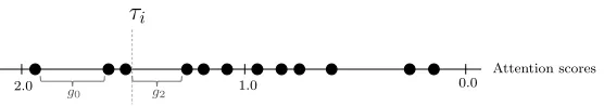
Figure 8: Threshold⌧j is set equal to the attention score at the left side of the largest gapgk wherek6= 0 andk <|G|/2. In this example⌧j is set equal to the third attention score.

attention scores from high to low and searches for the largest gap g between two adjacent attention scores ai,j and ak6=i,j, such that a split can be made between ‘high’ scores and ‘low’ scores. Threshold ⌧j is set equal to the attention score on the left side of the gap. This approach is graphically shown in Figure 8. We denote byGthe list of gaps [g0, ..., gN 1].

However, we have set three requirements for determining ⌧j (in priority order). First, we require that ⌧j 1, since all scores are initiated as 1 and a score will only be increased through backpropagation if the network attends to that corresponding time series. Secondly, since a temporal causal graph is usually sparse, we require that the gap selected for⌧j lies in the first half ofG(ifN >3) to ensure that the algorithm does not include low attention scores in the selection. This means that at most 50% of the input time series can be correlated with target Xj. By defining this requirement, we ensure that not too many time series are labeled ascorrelated. Although this number can be changed by the user, we experimentally estimated that 50% gives good results in the evaluation of our framework.

Lastly, we require that the gap for ⌧j cannot be in first position (i.e. between the highest and second-highest attention score). This requirement ensures that the algorithm does not truncate scores to zero of time series which were actually correlated, but weaker than the top scoring one. This means that at least 2 time series will be labeled ascorrelated for targetXj.

After ⌧j is determined, the HardSoftmax function can be applied. Thus, time series Xi is labeled as correlated with the target time seriesXj ifai,j2aj >⌧j, i.e. ifhi,j2hj>0. By applying HardSoftmax to the attention scores of allN networks, TCDF collects all correlations between time series discovered by the attention mechanisms.

4.2 Causal Validation

The second step of TCDF distinguishes causation from correlation. Recall that a causal relationship should comply with two aspects [Eichler, 2012]:

1. Temporal precedence: the cause precedes its e↵ect,

2. Physical influence: manipulation of the cause changes its e↵ect.

Since we use a temporal convolutional network architecture, there is no information leakage from future to past. Therefore, we already comply with the temporal precedence assumption. To comply with the second assumption, we have to validate that a change in a potential cause will influence its e↵ect. Since our method will be purely based on observational data, TCDF does not have the possibility to do a real-life experiment to check for physical influence. We therefore came up with a novel causal validation approach that uses only the observational dataset.

(29)

4.2.1 Attention Interpretation

After each networkNjis trained for an equal number of training epochs, the HardSoftmax attention scoreshj for each networkNj are collected to distinguish causation from correlation. By interpreting these attention scores, we can create a set of potential causes Pj for each time series Xj 2 X. This set Pj will serve as input for the CQII measure discussed in the next section.

We can observe the following cases between HardSoftmax scoreshi,j andhj,i:

1. hi,j= 0 andhj,i= 0: Xi is not correlated withXj and vice versa.

2. hi,j= 0 andhj,i>0: Xj is added toPi sinceXj is a potential cause ofXi because of:

(a) (In)direct causal relation fromXj to Xi, or

(b) Presence of a (hidden) confounder between Xj andXi where the delay from the confounder to

Xj is smaller than the delay toXi.

3. hi,j>0 andhj,i= 0: Xi is added toPj sinceXi is a potential cause ofXj because of:

(a) (In)direct causal relation fromXi toXj, or

(b) Presence of a (hidden) confounder between Xi and Xj where the delay from the confounder to

Xi is smaller than the delay toXj.

4. hi,j>0 andhj,i>0: Time series Xi andXj are correlated because of:

(a) Presence of a 2-cycle whereXi causesXj andXj causesXi, or

(b) Presence of a (hidden) confounder with equal delays to its e↵ectsXi andXj.

Note that a HardSoftmax score>0 could also be the result of a spurious correlation. However, since it is impossible to judge whether a correlation is spurious purely on the analysis of observational data, TCDF does not take the possibility of a spurious correlation into account. After causal discovery from observational data, it is up to a domain expert to judge or test whether a discovered causal relationship is correct. Section 6 presents a more extensive discussion on this topic.

By comparing all attention scores, we create a set of potential causes for each time series. Then, we will use the CQII measure to validate if a potential cause is a true cause. More specifically, TCDF will apply CQII to distinguish between case 2a and 2b, and between case 3a and 3b.

One could also use the CQII measure to distinguish between case 4a and 4b. In that case,Xi should be added toPj andXj should be added toPi. However, when we expect that a 2-cycle is non-existent (or at least sparse) based on domain knowledge, TCDF assumes that only the much more common case 4b occurs in order to save computational costs.

4.2.2 Causal Quantitative Input Influence

To allow for causal reasoning, we apply theCausal Quantitative Input Influence (CQII) measure

of [Datta et al., 2016] as described in Section 2.2. This measure models the di↵erence in the “quantity of interest” between the real input distribution and an intervened distribution. In our case, the quantity of interest is the loss_Lof the network between the predictions and the actual values of the target time series. As intervention, we change the input values of potential cause Xi 2Pj to random values having the same mean and standard deviation as the true values of Xi. Thus, the ‘real input distribution’ is the original input data, while the ‘intervened distribution’ is the input data where the intervention is applied.

Network_N0

jis then trained with the same input dataset as forNj, except thatXiis replaced with random values having the mean and standard deviation asXi. IfXi would be a real cause ofXj, the predictions of N0