Performance evaluation of a two-dimensional lattice Boltzmann solver using CUDA and PGAS UPC based parallelisation

(1)

39 Performance evaluation of a two-dimensional lattice Boltzmann

solver using CUDA and PGAS UPC based parallelisation

MÁTÉ SZŐKE,

University of Bristol

TAMÁS ISTVÁN JÓZSA,

University of Edinburgh

ÁDÁM KOLESZÁR,

Soliton Systems Europe

IRENE MOULITSAS and LÁSZLÓ KÖNÖZSY,

Cranfield University

The Unified Parallel C (UPC) language from the Partitioned Global Address Space (PGAS) family unifies the advantages of shared and local memory spaces and offers a relatively straight forward code parallelisation with the Central Processing Unit (CPU). In contrast, the Computer Unified Device Architecture (CUDA) development kit gives a tool to make use of the Graphics Processing Unit (GPU). We provide a detailed comparison between these novel techniques through the parallelisation of a two-dimensional lattice Boltzmann method based fluid flow solver. Our comparison between the CUDA and UPC parallelisation takes into account the required conceptual effort, the performance gain, and the limitations of the approaches from the application oriented developers’ point of view. We demonstrated that UPC led to competitive efficiency with the local memory implementation. However, the performance of the shared memory code fell behind our expectations, and we concluded that the investigated UPC compilers could not treat efficiently the shared memory space. The CUDA implementation proved to be more complex compared to the UPC approach mainly because of the complicated memory structure of the graphics card which also makes GPUs suitable for the parallelisation of the lattice Boltzmann method.

CCS Concepts: •Computing methodologies→Parallel computing methodologies;Modelling and simulation; •Applied computing→Physical sciences and engineering; •Mathematics of comput-ing→Mathematical software performance;

Additional Key Words and Phrases: artitioned Global Address Space, PGAS, Unified Parallel C, UPC, nVidia, Compute Unified Device Architecture, CUDA, Computational Fluid Dynamics, CFD, lattice Boltzmann method, LBM

ACM Reference format:

Máté Szőke, Tamás István Józsa, Ádám Koleszár, Irene Moulitsas, and László Könözsy. 2017. Performance evaluation of a two-dimensional lattice Boltzmann solver using CUDA and PGAS UPC based parallelisation.

ACM Trans. Math. Softw.99, 44, Article 39 (May 2017),22pages. DOI: 0000001.0000001

Author’s addresses: M. Szőke, Faculty of Engineering, University of Bristol, UK; T. I. Józsa, School of Engineering, University of Edinburgh, UK; Á. Koleszár, Soliton Systems Europe A/S, Taastrup, Denmark; I. Moulitsas and L. Könözsy, Computational Engineering Sciences, Cranfield University, UK..

Permission to make digital or hard copies of all or part of this work for personal or classroom use is granted without fee provided that copies are not made or distributed for profit or commercial advantage and that copies bear this notice and the full citation on the first page. Copyrights for components of this work owned by others than ACM must be honored. Abstracting with credit is permitted. To copy otherwise, or republish, to post on servers or to redistribute to lists, requires prior specific permission and/or a fee. Request permissions from [email protected].

ACM Transactions on Mathematical Software, Vol. 99, No. 44, Article 39. Publication date: May 2017. Volume 44 Issue 1, July 2017, Article No. 8

DOI:10.1145/3085590

(2)

1 INTRODUCTION

In the world of High Performance Computing (HPC), the effective implementation and paralleli-sation are vital for novel scientific software. Computational Fluid Dynamics (CFD) targets fluid flow modelling, which is a typical application field of HPC. While the Message Passing Interface (MPI) (Message Passing Interface Forum 2012) has become the dominant technique in parallel computing, other approaches, like the Partitioned Global Address Space (PGAS) (PGAS 2015) and the General-Purpose Computing on Graphics Processing Units (GPGPU), reared their heads in the last decade.

Co-Array Fortran (Numrich and Reid 1998), Chapel (Chamberlain et al. 2007), X-10 (Ebcioglu et al. 2004), Titanium (Yelick et al. 1998) and Unified Parallel C (UPC) (Chauwvin et al. 2007) are members of the PGAS model family. These languages attempt to offer an easier way for parallel programming on multi-core Central Processing Units (CPU) based systems compared to MPI. This involves keeping the code (a) portable: optimisation is made by the compiler in terms of architecture; (b) readable and productive: such languages were shown to be easier to code and easier to read (Cantonnet et al. 2004); (c) well performing: it was shown that such languages offer the same or even better performance than MPI (Johnson 2005;Mallón et al. 2009).

Performance-centred investigations were carried out to compare commercial UPC compilers (IBM, Cray, HP) with open source UPC compilers (GNU, Michigan, Berkeley).Husbands et al.(2003) reported that Berkeley UPC (BUPC) is competitive with the commercial HP compiler. The former achieved high performance in pointer-to-shared arithmetic because of its own compact pointer representation.

Mallón et al.(2009) compared UPC to MPI. They found that UPC showed poor results in collective performance against MPI (Taboada et al. 2009) due to high start-up communication latencies. In other aspects, their UPC code performed better than MPI.

Zhang et al.(2011) implemented the Barnes-Hut algorithm in UPC. They reported that the problem can be conveniently approached in UPC because the algorithm has dynamically changing communication patterns that can be handled by the implicit communication management of UPC. They reported poor performance because of the lack of efficient data management when their code relied on shared memory. The problem was resolved with the help of additional language extensions and optimisations ensuring that the data is cached accordingly from the global memory prior to it is requested.

Most of the performance evaluations were done via synthetic benchmarks such as FFT calcula-tions, N-Queens problem, NAS benchmarks from NASA (El-Ghazawi et al. 2006) etc., and only a limited number of papers focused on the application of UPC for physical problems. One of these is the work ofMarkidis and Lapenta(2010), where a particle-in-cell UPC code was implemented to simulate plasma. They experienced performance degradation for a high number of CPUs, the effect was dedicated to a specific part of their solver.

Johnson(2005) used Berkeley UPC compiler for an in-house code on a Cray supercomputer (Cray Inc. 2012) to run CFD simulations. Their code solved the incompressible Navier-Stokes Equations (NSE) using the finite element method. The UPC code showed better performance than the MPI version. The performance difference was bigger for a higher number of CPUs: UPC performed better than MPI, especially above 64 threads. It was shown that MPI required more time to pass small sizes of messages than UPC. Above a certain message size, UPC still performed better but the difference was negligible.

Although HPC centres are dominated mainly by multi-core CPUs, researchers discovered the potential for scientific computing on Graphics Processing Units (GPU) in the early 2000s ( McClana-han 2010). The Compute Unified Device Architecture (CUDA) Software Development Kit (SDK)

(3)

was released to popularise GPGPU on nVidia graphical cards (Sanders and Kandrot 2010). The CUDA libraries can be added to several languages, along with Fortran, Java, Matlab and Python, but most of the time it is used with C/C++. The essentially parallel nature of the graphical cards proved to be applicable in several fields, from pure mathematics (Manavski and Valle 2008;Zhang et al. 2010), through image processing (Stone et al. 2008), to physics (Anderson et al. 2008), including fluid flow modelling (Chentanez and Müller 2011;Ren et al. 2014).

The lattice Boltzmann method has become quite popular on parallel architectures because of the local nature of the operations which is discussed in Section2. The first parallel solvers were relying on CPUs, and were reported in the 1990s (Amati et al. 1997;Kandhai et al. 1998). Later on, GPU architectures were proven to be a good basis to parallelise the LBM. Two-dimensional CUDA implementation was published byTölke(2010), where a speedup of≈20 was reported. Several descriptions of three-dimensional solvers can be found, such asRyoo et al.(2008), where a speedup of 12.5 was measured.Rinaldi et al.(2012) reached a speedup of 131 using advanced strategies with CUDA. The LBM solver was proved to be highly efficient in multi-GPU environment as well (Xian and Takayuki 2011). As far as the authors know, onlyValero-Lara and Jansson(2015) considered using UPC for the LBM.

The advantages of the LBM are its good scalability, explicit time step formulation, applicability for multiphase flows (Succi 2001) and applicability for flows with relatively high Knudsen number (Mohamed 2011). The latter one is one of the main limitations of the NSE. The LBM has been developed for incompressible subsonic flows, it has second order of accuracy, and relatively high memory requirements due to the discretisation of particle directions.

In this paper, we present and compare the performance gain achieved after the CUDA and UPC parallelisation of an in-house LBM code. The solver handles two-dimensional fluid flow problems using the LBM. The comparison of the two currently applied architectures is not widely discussed from the performance point of view. Since HPC is often used by mathematicians, physicists, and engineers with limited computer science knowledge, we also aim to inspect how user-friendly CUDA and UPC are. We investigated the effect of the following factors:

a memory structure of UPC: shared and local variables;

b spatial resolution;

c hardware;

d collision models;

e data representation: single and double precision;

f required programming effort for the different codes.

The UPC implementation was evaluated on two different clusters, and the results were compared to the CUDA parallelisation on two different architectures. To quantify the performance the speedup was defined asSU =tserial/tparallel, wheretserialis the execution time of the serial code andtparallelis

the execution time of the parallel code.

2 THE IMPLEMENTATION OF THE LATTICE BOLTZMANN METHOD

The Boltzmann equation was derived to describe the motion of a large number of particles on a statistical basis. The idea behind the LBM is to discretise the Boltzmann equation so that particle propagation is allowed only in certain discrete directions. The governing equation is written as Eq. (1), wheref =f( ®x,p®,t)is the distribution function, which represents the probability of “finding a molecule around positionx®at timetwith momentump®” (Succi 2001).c®is the microscopic particle velocity, andΩ=Ω(f)is the collision operator. The Chapman-Enskog procedure forms a clear bridge between the LBM equation (1) and the NSE (in the artificial compressibility form proposed

(4)

byChorin(1967)), thus the method can be used to describe incompressible fluid flows (He and Luo 1997).

∂f

∂t +(®c· ∇)f =Ω (1)

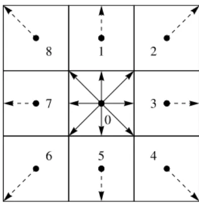
We applied the D2Q9 model, which means that the resolved flow field was two-dimensional, and particle propagation was allowed in nine discrete directions (Fig.1). The time marching was divided into four steps from the implementation point of view:

I. Collision The collision modelling treats the right hand side of Eq. (1). Two collision models were analysed:

a In the BGKW model, the collision is described by Eq. (2) which was derived by Bhat-nagar et al.(1954) and byWelander(1954). Hereτ is the relaxation factor, calculated from the lattice viscosity of the fluid, andfeq_{is the so called local equilibrium}

distri-bution function described by the Maxwell-Boltzmann distridistri-bution (Maxwell 1860). It is important to note that the collision term can be computed independently for every direction after the discretisation as

Ω= 1

τ(feq−f). (2)

b The Multi Relaxation Time (MRT) model was presented and reviewed byd’Humières

(1992) andd’Humières et al.(2002). In this case, instead of using a single constant (τ−1) to describe the collision, the model applies a matrix which depends on the resolved directions (D2Q9). In our case, this matrix has a dimension of 9×9. This approach yields a matrix multiplication for each lattice. Despite the fact that this model is computationally more expensive than the BGKW, it is widely applied since the flow field can be more accurately resolved.

II. Streaming The streaming process occurs when the directional distribution functions “travel” to the neighbouring cells: second term on the left hand side of Eq. (1). This process

is presented in Fig.1(b).

III. Boundary treatment These steps are followed by the handling of the boundaries. In the current paper, the boundary description suggested byZou and He(1997) was used for the moving wall, and the so called bounce-back boundary condition (Succi 2001) was used to handle the no-slip condition at the stationary walls.

IV. Update macroscopic Once the distribution functions were known at the end of the time step, the macroscopic variables (density, x- and y-directional velocity components) had to be computed from the distribution functions to recover the flow field.

The sum of the listed items is referred from now on as themain loop. The grid generations and the initialisation of the microscopic and macroscopic variables took place before themain loop.

In terms of the computational grid, the method is based on a uniform Cartesian lattice, which is represented in Fig.1(a), where the nine directions of thestreamingare displayed as well. In order to examine the effect of the spatial resolution on the performance gain, four different grids were investigated. In the following, the lattices are referred to based on the names given in Table1.

The simulated fluid flow was the well known lid-driven cavity, which is a common validation case for CFD solvers (Ghia et al. 1982). The aspect ratio of the domain was unity. The lid on the top moved with a defined positive x-directional velocity, while all the other boundaries were stationary walls (see Fig.1(a)). From these conditions, the Reynolds number in the domain was defined based on the lattice quantities asRe =nxulid/νl, wherenx =nis the number of lattices along the x-direction,ulidis the lid velocity, andνl is the lattice viscosity, which was set to be 0.1.

(5)

Wall

Lid

x

y

u

_lid

(a) Lattice and the applied boundary conditions

0 1 2 3 4 5 6 7 8

(b)Streamingand the nine discrete directions (ci®)

Fig. 1. Structure of the computational domain

Table 1. Applied mesh sizes

Name Size Lattices

nx ×ny

Coarse 128×128 16,384

Medium 256×256 66,536

Fine 512×512 262,144

Ultra Fine 1024×1024 1,038,576

The Reynolds number of the simulations was 1000. At the end of the computations, the coordinates and the macroscopic variables were saved. A qualitative validation of the flow field can be found in AppendixB. For a more comprehensive validation and verification, we refer to the work ofJózsa et al.(2016).

3 PARALLELISATION

The serial code was written in C, and the code was built up as it was presented in Section2. The serial implementation was based on one-dimensional Array of Structures (AoS), similarly to the UPC version. TheCellsstructure included the macroscopic variables (velocity components asUand V, density asRho, etc.) as scalars, while the distribution functionFwas stored as a nine-dimensional array within theCellsstructure. Thus(Cells+i)->F[k]referred to theithlattice in the domain and the corresponding distribution function in thekthdiscrete direction. The parallelisation process can be followed in AppendixA. The serial simulations were performed on Archer, the United Kingdom National Supercomputing Service.

(6)

Table 2. Properties of the used CPU clusters

Properties Astral (Intel) Archer (Cray)

Compiler BUPC Cray C

Intel processor number E5-2660 E5-2697

Processor clock rate [GHz] 2.2 2.7

Processors per node 2 2

Threads per processor 8 12

Threads per node (used) 16 (16) 24 (16)

Memory per node [GB] 64 64

Cache per processor [MB] 20 30

Interconnect type Infiniband Cray Aries

Recommended customer pricea $1445 $2890 a_{Prices as of 12/2016.}

First, we parallelised the solver with UPC and ran the codes on Archer and Astral. The latter is the HPC cluster of Cranfield University. The hyper-threading technology (Intel 2015) was switched off on both architectures. The properties of the two clusters are listed in Table2. A higher performance can be expected on Archer since it holds several optimisation properties such as hardware supported shared memory addressing. Note that the interconnection between the nodes are different in the two investigated clusters. On Archer the commercial Cray C compiler was available, while the open source BUPC compiler was installed on Astral.

Second, the CUDA parallelisation was tested. The performance gain was evaluated on two different nVidia GPUs. The relevant properties of the graphical cards are listed in Table3. While the GeForce cards are cheaper devices, as they are primarily designed for computer games, the Tesla cards are more expensive, directly designed for scientific computing. The code development was carried out on a desktop using the GTX 550Ti card, while the Tesla GPU of the University of Edinburgh‘s Indy cluster was used for further investigations.

Table 3. Properties of the used GPUs

Properties GeForce GTX 550Ti Tesla K20

CUDA release v7.5 v6.0

Number of CUDA cores 192 2496

Global memory type GDDR5 GDDR5

Global memory bandwidth [GB/s] 98.5 208

Global memory size [GB] 1 5

Single precision performance [GFLOPs] 691 3524

Double precision performance [GFLOPs] unknown 1175

Recommended customer pricea _$230 _$2300

a_{Prices as of 12/2016.}

3.1 Unified Parallel C Approach

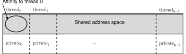
UPC is an extension of the standard C language but it requires its own compiler. The novelty of UPC relies on its memory structure, where the user has the opportunity to lay down variables in

(7)

the shared address space and in the local memory at the same time. A schematic draw of the local and the shared memory spaces is showed in Fig.2. Implementing UPC based codes therefore offers the opportunity to combine the advantages of the conventional parallelisation methods, such as OpenMP and MPI, whose restrict the programmer to rely purely on either shared or local memory only. The UPC compiler is designed to manage and handle the data layout between the threads and nodes. This keeps the architecture based problems hidden from the user, i.e. optimisation is expected to be performed by the compiler.

Fig. 2. Memory model of the local and shared memory spaces (Chauwvin et al. 2007)

The syntax of the local memory declarations is the same as in the standard C language. Data exchange between the threads is performed via theupc_memput,upc_memgetandupc_memcpy functions. The first function copies local data to the shared space, and the second copies data from the shared to the local memory. The last function performs data copy from shared to shared address space. Note that the first and second functions are similar to theMPI_SendandMPI_Recvfunctions. The shared memory based data needs to be declared according to the UPC standards. In this case, the programmer must declare a compile time constant block size, which defines how many elements of a vector belongs to each thread. The data is laid down between the threads with a round-robin fashion using the corresponding block size. We can see that the compile time constant restriction is the biggest drawback of the investigated language. If the programmer wishes to lay down the whole mesh, for example here in the shared memory, then the mesh size needs to be known in advance of the compilation. In other words, different executable files are needed for different mesh sizes.

To perform shared memory based operations, UPC offers the usage ofupc_forall, which is an extension of the standard Cforloop. Each shared variable within a vector has an affinity term that describes which thread the given element belongs to. Based on this information, theupc_forall distributes the computational load between the threads. UPC also offers the usage of barriers, locks, shared pointers, collectives etc. For further description we refer toChauwvin et al.(2007).

In our case, two UPC codes were implemented: (a) one with shared memory implementation, and (b) another code relying on the local memory. Thestreamingstep of these codes are given as an example in AppendixA. In the former code, the data is laid down in the shared memory, and in the latter one, the data is stored in the local memory. The shared memory based code exploits the novelty of UPC, i.e. this code relies on theupc_forallfunction and shared pointer declarations. This leads to a more easily readable code. The second approach, which exploits data locality and follows the logic of MPI implementations, offers better speed and lower latency time. As a disadvantage, theupc_memput,upc_memgetmemory operations were required; therefore this code is more complex and consists of more lines. The computational load was distributed equally between the threads in both implementations, since the mesh size was divisible by the number of threads during the simulations.

During the compilation of the UPC codes, similarly to the serial code, the performance affecting flags were avoided. The compile command of the UPC codes, for example using four threads, was

(8)

upcc -T=4 *.c -lm -o LBMSolver. The execution simplified toupcrun LBMSolveron both HPC systems.

3.2 nVidia CUDA

The CUDA SDK contains several additional functions to make the programming of nVidia GPUs possible. The programming of the graphical card, from now referred to as ‘device’, requires some basic knowledge of its structure. The working units are the so called threads, which form separate blocks. Theoretically, every thread can work in parallel. Originally the threads could perform operations only on the data which was stored in the device memory. This meant that the programmer had to work out the data transfer between the host and device memory. The most recent solution of nVidia to bridge this problem is the unified memory (available since v6.0), which enables automatic data migration between the host and the device. Nevertheless, the host memory bandwidth is evidently the bottle neck of the available performance gain. It is a rule of thumb that the data transfer between the host and the device should be minimised for high efficiency.

After the data has been copied to the device, CUDA offers an opportunity to manage the multilayer memory structure of the GPUs. In the current study, only the global and the constant memories were used. When data is copied to the device, it is stored originally in the global memory (Table3). Every thread has access to this data, however this memory has the smallest bandwidth on the device. To quicken the speed of the calculations, the parameters can be stored in the constant memory which has a higher bandwidth but a smaller size.

The shared memory capability becomes increasingly important when the communication be-tween the blocks is high. For instance, in the case of the so called prefix sum, when every element of a vector are summed. Originally, the threads within different blocks can communicate only through the relatively slow global memory. However, the threads have access to the shared memory only within the blocks, the appropriate management of this memory layer often leads to significant performance gain because of its high bandwidth and low latency. For further description on the memory structure of the GPU and on CUDA programming we refer toNickolls et al.(2008) and

Sanders and Kandrot(2010).

The CUDA parallelisation included the following main steps (presented through thestreaming

in AppendixA):

CUDA 1 Several smaller structures were used instead of theCellsstructure, for example Cells_var_9d_dto store the nine-dimensional distribution functions (AppendixA, CUDA parallelisation step 1). The inefficientforloops were avoided, so that thestreamingwas performed theoretically in parallel for every node in every discrete direction.

CUDA 2 The so called structures of array (SoA) approach was implemented, which proved to be more efficient compared to the AoS approach (Ryoo et al. 2008). This means that every variable (e.g. density and velocity components) was stored in separate one-dimensional arrays. This SoA version of the code proved to be≈5 times faster than the AoS version. The maximum speedup with this implementation, measured with the ultra fine lattice on the Tesla K20 card using SP, was≈20. This is similar to the speedup achieved byTölke(2010) on a 2D lattice, but seems infinitesimal compared to the 131 speedup reported byRinaldi et al.(2012) using a 3D domain.

CUDA 3 The SoA approach was kept but the threads were assigned to the lattices and the discrete directions were taken step by step as it is shown in AppendixA. We note that the operations related to the 0thdiscrete direction were ignored during thestreamingin the last version of the CUDA code because they do not have any physical role. This simplification did not influence the performance significantly.

(9)

After theboundary treatmentwas identified as the bottleneck of the computations (see Section4, Fig.6), the global search, which was performed based on a boolean mask at every time step to find the boundary lattices, was replaced. In the last version the boundary lattices were selected during the initialisation so that theboundary treatmentkernel function “knew” the location of the boundaries in advance.

In every case, one-dimensional grids and blocks were used; furthermore 256 threads were initialised within every block (block size). The number of the blocks (grid size) varied automatically as a function of the mesh size. This set-up proved to be the most efficient computationally, although it resulted in a strong limitation in terms of the maximum mesh size. The theoretical maximum thread number of the devices is 65535×1024 (maximum grid size times maximum block size). In the first two implementations the threads were assigned to every distribution function in every lattice which led to a maximum cell number 65535×256/9≈1864207. This limitation was overcome in the third CUDA parallelisation step by assigning the threads to the cells. This way the maximum number of lattices was nine times higher.

The last version of the CUDA code was compiled with thenvcc -arch=sm_20 -rdc=true command. Here the first flag defines the virtual architecture of the device, while the second one allows the user to compile the files separately and link them at the end. (The first and the second version did not need the-rdc=trueflag, since the kernel functions were in one file.) The authors note that compiling the code with a more recent virtual architecture for the K20 GPU, for instance -arch=sm_35, would probably result in an enhanced parallel performance. The-arch=sm_20flag was used because this was the most recent virtual architecture supported by both of the tested GPUs. The detailed analysis of the code performance can be found in Section4.

4 RESULTS AND DISCUSSION

In this section, we will discuss the achieved speedup of themain loop. Firstly, the serial results will be analysed. Secondly, the UPC approaches will be evaluated. Finally, the nVidia CUDA parallelisation will be examined and compared to the UPC approaches. In addition we will evaluate the applied parallel approaches from the code developer’s point of view.

4.1 Serial simulations

The measured iteration times of the serial simulations are listed in Table4. As expected, the simulation time increased with the grid size. A factor of approximately four can be identified between the computational cost of the coarse-medium and fine-ultra fine grids, which is logical since the grid size increased exactly by the same factor. This observation is not valid between the medium and fine meshes. While the variables for the coarse and the medium mesh can be fitted into the cache, the memory requirement of the fine and the ultra fine meshes exceeds the cache size. As we expected, the MRT model was computationally more expensive than the BGKW. Compared to the BGKW model, the MRT execution time was typically 10–50% higher, and as the number of cells increased the MRT model became relatively cheaper.

4.2 Performance analysis of the UPC codes

The shared and local approaches were compared in terms of the achieved speedup in Fig.3. The dash-dotted line shows the theoretical limit, the linear speedup (SU =Nthreads) in all figures presented in

the current subchapter. Fig.3(a)presents the shared memory based speedup achieved on Astral and Archer using the fine mesh and double precision. We can see that the shared memory based code led to poor parallel performance. By using any number of threads, the gained performance was far below the linear speedup. Furthermore, for lower number of threads (4 and 8), the parallel

(10)

Table 4. Wall time per iteration, serial simulations[ms] Grid

Collision model Precision Coarse Medium Fine Ultra fine

BGKW Single 1.204 4.974 45.01 177.6

BGKW Double 1.264 9.664 59.77 240.5

MRT Single 1.696 7.092 51.56 204.1

MRT Double 1.956 11.946 65.75 263.1

code was slower than the serial. By crossing nodes, the speedup continued to increase indicating appropriate communication between the nodes.

48 16 32 64 128 4 8 16 32 64 Threads [−] Speedup [−] Astral, BGKW Astral, MRT Archer, BGKW Archer, MRT Linear Speedup

(a) Shared memory approach

48 16 32 64 128 4 8 16 32 64 128 Threads [−] Speedup [−] Astral, BGKW Astral, MRT Archer, BGKW Archer, MRT Linear Speedup

(b) Local memory approach

Fig. 3. speedup of themain loopas a function of the parallelisation approach, fine mesh, double precision arithmetic

Fig.3(a)indicates that none of the simulations exploit the maximum performance of the su-percomputers. Despite the hardware support of the shared memory operations on Archer, the simulations did not show better speedup results compared to Astral. We hypothesised that the compilers could not handle the shared pointers and manage the data between the shared and local memory spaces effectively. As a first step, performance analysis was conducted on Archer using CrayPat (Cray 2015), which showed that the data was managed and “fed” to the CPUs properly.

As a next step, we tried to find other reasons for the problem. We reckon that the poor performance might have been caused by one of the following factors, and so we took measures to overcome them:

a usage of shared pointers. All of them were tested with static variables;

b inappropriate time measurement. We tested different approaches such as theclock(), and theMPI_Wtime()commands;

c inappropriate usage of theupc_forallcommand. Different methods were examined to distribute the computational load, for instance working threads were defined based on affinity of shared variables (&Cells[i]) or modular division of integers (i % THREADS);

(11)

d usage ofCellsstructure. The structure was eliminated (see the code samples in AppendixA);

e lack of optimisation flags. All of the available optimisation flags (-O1, -O2, -O3) were tested. None of these modifications resulted in better speedup in the case of shared variables, i.e. the experienced performance of the shared code was the same for each listed factors. Therefore, we concluded that the compiler cannot handle the data properly without additional modifications, and for this particular application the compiler is still not mature enough. As it was presented by

Zhang et al.(2011), the problem could be resolved by outer libraries and user implemented machine level data management. Adding these low level modifications to the shared code would eliminate the main advantage of UPC, namely the quick and user-friendly parallelisation environment. To overcome this problem the data was rather transferred to the local memory and another, MPI-like code was developed.

48 16 32 64 128 4 8 16 32 64 128 Threads [−] Speedup [−] Astral, BGKW Astral, MRT Archer, BGKW Archer, MRT Linear Speedup

(a) Local memory based speedup, single precision arith-metic 48 16 32 64 128 4 8 16 32 64 128 Threads [−] Speedup [−]

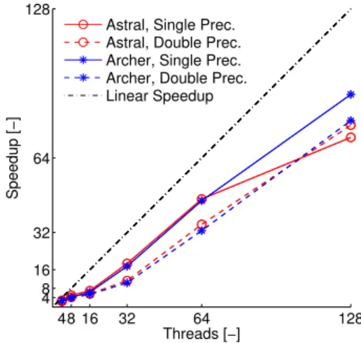
Astral, Single Prec. Astral, Double Prec. Archer, Single Prec. Archer, Double Prec. Linear Speedup

(b) Comparison of double and single precision speedup, MRT collision model

Fig. 4. Main loopspeedup results on fine mesh

Fig.3(b)shows the local memory based speedup using the fine mesh and double precision. This approach gave significantly better results. Here we can see that crossing a node did not introduce significant latency either, the compilers were capable of managing the halo swap between the nodes.

Fig.4(a)shows the speedup as a function of the collision model. The two models had similar parallel efficiency. We can see that the BGKW collision model (solid lines) enabled slightly better speedup results than the MRT collision model. Fig.4(b)gives us a basis for an explicit comparison between the performance of the single and double precision executions. This graph shows the speedup achieved on the fine mesh with the MRT collision model. We can see that the single precision results (continuous lines) are better above 16 threads than the double precision ones (dashed lines). Between 16 and 32 threads the first node was crossed on both architectures. The difference between the single and double precision curves above 16 threads are originated from the communication costs. The double precision approach requested more data handling resulting in lower speedup.

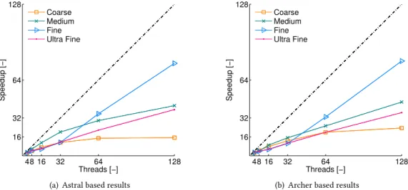
We plotted the effect of mesh size on the speedup in Fig.5(a)and5(b)for Astral and Archer, respectively. If we consider more than 32 threads, then we may conclude that better speedup were

(12)

achieved with increasing mesh size. Unexpectedly, this finding was not valid for the ultra fine mesh, where performance degradation was experienced on both architectures. To find the “leakage” in the performance we measured the time spent with the data transfer on the fine and the ultra fine meshes using 128 threads. With this set up, the halo included twice as much data on the ultra fine mesh than on the fine mesh, so that the data transfer should take roughly twice as long as well. In contrast, the data transfer took six times longer on the ultra fine mesh compared to the fine. The performance degradation experienced on the ultra fine mesh was caused by the increased communication costs, which seems to be a relatively strong limitation. We note that the ultra fine mesh consists of approximately one million cells, so the computational load of the processors is still reasonably low when 128 threads are allocated.

48 16 32 64 128 16 32 64 128 Threads [−] Speedup [−] Coarse Medium Fine Ultra Fine

(a) Astral based results

48 16 32 64 128 16 32 64 128 Threads [−] Speedup [−] Coarse Medium Fine Ultra Fine

(b) Archer based results

Fig. 5. The effect of mesh size on themain loopspeedup, double precision number representation

4.3 Performance comparison of the UPC and CUDA codes

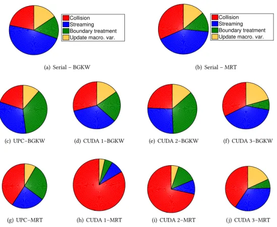
In this subsection only the local memory based UPC implementation run on 64 threads will be analysed and compared to the serial and CUDA simulations. Fig.6shows profiling results of the different codes. Based on Figs.6(a)and6(b)one can identify thecollisionand thestreamingas the most expensive operations. We can conclude from these two figures that the MRT model is slightly more expensive than the BGKW model. Although theboundary treatmentis relevant only for the nodes on the perimeter of the domain, it still needs approximately as much time as theupdate

macroscopicoperation, because the boundary nodes are treated based on a global search.

Compared to the serial results, the UPC implementation drew attention to the the inefficient

boundary treatmentwhich became one of the most expensive operation in the UPC approach

(Figs.6(c)and6(g)). Furthermore, the parallelisation highlighted the increased cost of thecollision

in the MRT model, which was more expensive compared to the other steps (Fig.6(g)).

The MRT collision model was found to be computationally more expensive on the GPU as well. We can see how thecollisionstep became less expensive during the development (Figs.6(h),6(i) and6(j)), although it still took approximately 40% of themain loop. The MRT model includes summations along the discrete directions. In the first and the second CUDA development steps these summations required operations between the blocks, while in the final version the summation

(13)

Collision Streaming Boundary treatment Update macro. var.

(a) Serial – BGKW

Collision Streaming Boundary treatment Update macro. var.

(b) Serial – MRT

(c) UPC–BGKW (d) CUDA 1–BGKW (e) CUDA 2–BGKW (f) CUDA 3–BGKW

(g) UPC–MRT (h) CUDA 1–MRT (i) CUDA 2–MRT (j) CUDA 3–MRT

Fig. 6. Profiling results based on single precision simulations with fine mesh on the GTX 550Ti graphical card, and on Archer using 64 threads

happened within the blocks, so that it could be done more efficiently. While the first and the second CUDA development steps were more favourable for thestreaming, the third step was specifically developed to decrease the cost of thecollision.

The scalability of the codes as a function of the hardware is displayed in the bar charts in Fig.7. As we can see in Figs.7(a)and7(b), the speedup of the BGKW and the MRT models were bounded around 50 on Archer, and around 80 on the Tesla K20 card. In case of the K20 card, the performance gap between double and single precision execution is clearly visible: while a maximum speedup of around 80 was measured with single precision arithmetic (Fig.7(a)), a speedup around 65 could be achieved with double precision arithmetic in the case of the BGKW model (Fig.7(c)). A similar trend can be seen in the case of the MRT model as well, with a slightly wider gap between the single precision and double precision arithmetic (Figs.7(b)and7(d)). Considering that the double precision processing power of the K20 unit is approximately a third of its single precision processing power (Table3), it might seem surprising that the performance gap is only around 20%. If we also consider that two of the main steps in the LBM, (streamingandboundary treatment) are essentially data copying, then the relatively small gap makes more sense: the high memory bandwidth of the GPU compensated for the lack of computing power.

(14)

Coarse Medium Fine Ultra fine Grid 10 20 30 40 50 60 70 80 Speedup GTX550Ti Tesla K20 Archer 64 threads

(a) Single precision, BGKW

Coarse Medium Fine Ultra fine

Grid 10 20 30 40 50 60 70 80 Speedup GTX550Ti Tesla K20 Archer 64 threads (b) Single precision, MRT

Grid 10 20 30 40 50 60 70 80 Speedup GTX550Ti Tesla K20 Archer 64 threads (c) Double precision, BGKW

Grid 10 20 30 40 50 60 70 80 Speedup GTX550Ti Tesla K20 Archer 64 threads (d) Double precision, MRT

Fig. 7. Speedup of themain loopas a function of the grid spacing and the hardware

Interestingly, the GTX550Ti device showed better parallel performance with the MRT model compared to the BGKW model (Fig.7(a)and7(b)). While this card gave higher speedup with DP in the case of the BGKW model, using DP led to a drastic performance drop with the MRT model (compare Fig.7(a)with7(c)and Fig.7(b)with7(d)).

Based on the charts, the K20 card performed in almost every case better than the GTX550Ti. In fact, the K20 card was slightly slower than the GTX550Ti only when the grid size was small. In our case, the medium grid proved to be big enough to utilise the better potentials of the K20 GPU. As the grid size increased we could measure an increasing speedup in the case of the K20 device, while the GTX550Ti card reached its limits at the fine mesh. These results mirror the GPUs’ evolution, and correlate well with the hardware parameters (e. g. CUDA cores) given in Table3.

Ideally, in the case of the CPU parallelisation, when the number of threads is kept constant and the grid size changes, a nearly constant speedup can be expected. After looking at Fig.7, it becomes clear how far away this application is from an ideal situation: increasing the number of lattices up to a certain point (fine mesh), resulted in an increasing speedup. This happened because as the problem size increased, the time spent with the halo swap decreased relative to the time spent with the computation of the different operations. The speedup on Archer with 64 threads was close to the ideal when single precision arithmetic was used on the fine mesh (Figs.7(a)and7(b)). However,

(15)

Coll Str BT UM Operation 50 100 150 200 250 300 350 Speedup GTX550Ti Tesla K20 Archer 64 threads

(a) Single precision, BGWK

Coll Str BT UM Operation 50 100 150 200 250 300 350 Speedup GTX550Ti Tesla K20 Archer 64 threads (b) Single precision, MRT Coll Str BT UM Operation 50 100 150 200 250 300 350 Speedup GTX550Ti Tesla K20 Archer 64 threads (c) Double precision, BGWK Coll Str BT UM Operation 50 100 150 200 250 300 350 Speedup GTX550Ti Tesla K20 Archer 64 threads (d) Double precision, MRT

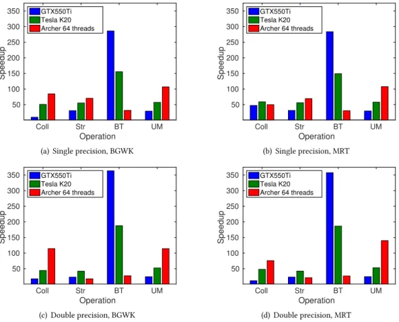
Fig. 8. Speedup of the different operations on the fine grid as a function of the hardware. (Coll–Collision; Str–Streaming; BT–Boundary treatment; UM–Update macroscopic)

using double precision arithmetic means an increased computational load for each threads, it also means increased communication between the threads. Probably this is the reason why the parallel performance of the double precision execution was lower on Archer compared to the single precision simulations when the fine mesh was investigated. (Figs.7(c)and7(d)).

In order to gain a better understanding of the results, deeper analyses of the code is required. The speedup of the main parts of the code are shown in Fig.8. It is important to recognize that, theoretically, only the speedup of thecollisionstep should change when we consider different models. Indeed, the other operations show only a small deviation (compare Figs.8(a),8(c)with8(b), 8(d)). After a first look, we can see that theboundary treatment, which was identified as the bottle neck of the performance (Fig.6), was significantly improved in the final step of the CUDA code. This high speedup was measured, because the global search of the boundaries was replaced (see Section3.2). Furthermore, it is also visible that the other parts of the code had a relatively uniform speedup in the case of the CUDA implementation: for the K20 card around 50 with single precision and 40 with double precision. When compared with the K20, the GTX550Ti device showed better speedup of theboundary treatmentbut a worse speedup of the other operations. The unexpected behaviour of the GTX550Ti card when compared to K20 can be caused by its structure which was designed for gaming, or the different CUDA release (see Table3).

(16)

The speedup of the operations measured on Archer shows less deviation. However, it was found that the measured speedup exceeded the theoretical limit (64) several times, especially for the

collisionand theupdate macroscopicparts, while other times the parallel code underperformed. This behaviour seems to be logical if we take into account that thecollisionand theupdate macroscopic

operations do not require any communication between the processes. Furthermore, the data of the partitioned mesh fit the cache of the nodes, while the same data exceeded the cache size of a single node in the case of the serial execution.

4.4 UPC and CUDA beyond performance

Because of the complex memory structure of the GPUs, the CUDA parallelisation was more cumbersome and time consuming. We can see that certain parts of the code (e. g.boundary treatment) needed significant reformulation in order to reach higher performance. Furthermore, it is important to note that for a CPU related parallelisation it is reasonably well understood how the efficiency can be improved, but for a complex application, like the current study, the CUDA related optimisation requires more conceptual effort and the identification of performance loss is more complex. All in all, the final version of the CUDA code required roughly twice as much working hours than the UPC parallelisation. The final code was achieved via three steps, and there are still several opportunities to further increase the performance, for instance, using the shared memory of the cards or multiple graphical cards.

Table 5. Number of lines in the different codes

Code Number of lines in implementation:

name Main loop Overall

Serial 1148 2215

UPC: Archer – Shared 1294 2413

UPC: Archer – Local 1359 2566

UPC: Astral – Shared 1294 2413

UPC: Astral – Local 1337 2629

CUDA: Step 1 1596 2455

CUDA: Step 2 1748 2547

CUDA: Step 3 1676 4684

Although the straightforward shared memory approach of UPC proved to be inefficient, the classical MPI-like local parallelisation technique gave acceptable results. Thanks to its simple syntax, it needed less programming effort compared to CUDA. The corresponding number of lines for the different codes are listed in Table5. We can see that the most efficient CUDA implementation took

≈40% more lines, while the longest UPC implementation needed only≈15% more lines compared to the serial code. It is arguable whether counting the number of lines is representative of the programming effort but in this case it is well correlated to the required work. The efficient paralleli-sation with CUDA required roughly twice as much office hours than the two UPC implementations. Without a doubt, we can conclude that the highest amount of conceptual effort was required by the CUDA approach followed by the local UPC code and the shared UPC code.

It is important to see what kind of compromises application oriented developers need to make. The situation can be described with the help of the triangle shown in Fig.9. The edges of the triangle contain the good properties of a high performance programming approach: low conceptual effort, high performance and low hardware costs. For the lattice Boltzmann method, the first possible

(17)

Fig. 9. Compromise triangle of high performance scientific programmers

scenario includes a low cost hardware (Tesla K20 of $2300) and a reasonably high performance but we have to pay the price of conceptual effort because of the GPU’s programming environment. Another extreme scenario is when a higher budget is available (Intel E5 processors, each for $2900), and we can work with a more flexible programming environment, and probably end up with an efficient code in a shorter period of time. This situation makes the local memory based UPC programming environment a suitable candidate. Additionally to these two cases, when the available budget is limited, one can consider running single core simulations on a cheap hardware. This would clearly require longer computations because of the low performance. The choice between the three scenarios is still usually made by the time frame, the available hardware, and skill set. However, the shared memory approach of UPC aims to provide another low effort, high performance scenario, our investigations highlighted that the compilers need further development to achieve this goal.

5 CONCLUSIONS

We parallelised an in-house, two-dimensional lattice Boltzmann solver using CPU and GPU paral-lelisation approaches. We presented the UPC implementation of the lattice Boltzmann method and compared the parallel efficiency of our CUDA and UPC codes using the two-dimensional physical problem of the lid-driven cavity. The UPC codes were tested with two different compilers on two different clusters, while the CUDA codes were run on two different GPUs. A detailed performance analysis of the different implementations was performed to provide an insight into the parallel capabilities of UPC and CUDA when it comes to the lattice Boltzmann method.

The parallelisation of thecollisionproved to be crucial since this is the part in the algorithm where the majority of the computation happens. Based on our experience the efficiency of this part determines the globally experienced efficiency, and it typically means favourable implementation for theupdate macroscopicoperation as well. We would like to draw attention to theboundary treatmentas well, since it can easily become the bottle neck of the parallel code, although its execution time is essentially limited by the memory bandwidth similarly to thestreaming.

The UPC code using the shared memory approach showed surprisingly low performance com-pared to the serial code. We found that the investigated compilers could not automatically manage the data transfer between the threads efficiently. The further development of the compilers may

(18)

solve this issue and make the UPC approach more user-friendly and attractive for future scientific programmers. Until then, we can enjoy the simple syntax of UPC for local memory based imple-mentation, which was proven to be more efficient and suitable for the parallelisation of the lattice Boltzmann method.

The CUDA development was presented through three different steps which highlighted that the used data structures (namely the AoS and the SoA approaches), and the data distribution strategies have a significant effect on the parallel performance. We can confirm that the nVidia graphics cards, especially the ones designed for scientific computing, are highly suitable for the parallelisation of the lattice Boltzmann method. Based on our measurements a single GPU might compete with 3-4 supercomputer nodes (around 80 threads) or more, for a significantly lower price. To reach this high performance developers need more specific skills and programming effort when it is compared to the local UPC implementation.

CODE AVAILABILITY

The developed codes are available as open source and can be downloaded from GitHub athttps: //github.com/mate-szoke/ParallelLbmCranfield. The codes are available under the MIT license. The folders also include all mesh and setup files used to perform the documented simulations. ACKNOWLEDGMENTS

This work used the ARCHER UK National Supercomputing Service (http://www.archer.ac.uk). The authors would like to thank the Edinburgh Parallel Computing Centre for providing access to the INDY cluster. We are also grateful for the ASTRAL support given by the Cranfield University IT team. Further thanks go to Tom-Robin Teschner and Anton Shterenlikht for useful discussions, Kirsty Jean Grant for the proofreading, and Gennaro Abbruzzese for the original C++ version of the code and the mesh generator which was used for our simulations.

A CODE SECTIONS

The following code sections cover thestreaming:

• Serial code

1 for ( i =0; i <(* m ) *(* n ) ; i ++) { // swe ep t h r o u g h the d o m a i n

2 if ( ( Cel ls + i ) -> Flu id == 1 ) { // if the l a t t i c e is in the fl uid d o m a i n

3 for ( k =0; k <9; k ++) { // s wee p a lon g the nine d i s c r e t e d i r e c t i o n s

4 // if s t r e a m i n g is a l l o w e d in the c u r r e n t d i r e c t i o n

5 if ( (( Cel ls + i ) -> S t r e a m L a t t i c e [ k ]) == 1) {

6 // the c u r r e n t dis tr . fct . t r a v e l s to the c o r r e s p o n d i n g n e i g h b o u r

7 ( C ell s + i ) -> F [ k ] = ( C ell s + i + c [ k ] ) -> MET AF [ k ];

8 } } } }

• UPC parallelisation relying on local pointer variables

1 for ( i = 0; i <( n _ s u b _ x * n _ s u b _ y ) ; i ++) { // swe ep in the who le sub - d o m a i n

2 if (( Cel ls + i ) -> Flu id == 1) { // if the l a t t i c e is in the fl uid d o m a i n

3 for ( k =0; k <9; k ++) { // s wee p a lo ng the nine d i s c r e t e d i r e c t i o n s

5 if ( (( Cel ls + i ) -> S t r e a m L a t t i c e [ k ]) ) == 1 ) {

7 ( C ell s + i ) -> F [ k ] = ( C ell s + i + c [ k ] ) -> M ET AF [ k ];

8 } } } }

(19)

1 u p c _ f o r a l l ( i =0; i <((* nx ) *(* ny ) ) ; i ++; & Flu id [ i ]) { // swe ep in the wh ole d o m a i n

2 if ( Flu id [ i ] == 1) { // if the l a t t i c e is in the fl uid d o m a i n

3 for ( k =0; k <9; k ++) { // s wee p a lo ng the nine d i s c r e t e d i r e c t i o n s

5 if ( S t r e a m L a t t i c e [ i ][ k ] == 1 ) {

7 F [ i ][ k ] = M ETA F [ i + c [ k ]][ k ];

8 } } } }

• CUDA parallelisation step 1,streamingkernel function

1 int bidx = b l o c k I d x . x ; // ind ex of the c u r r e n t blo ck

2 int tidx = t h r e a d I d x . x ; // ind ex of the c u r r e n t t h r e a d w i t h i n the blo ck

3 // g l o b a l ind ex of the t h r e a d s up to 9* nx * ny

4 int ind = tidx + bidx * b l o c k D i m . x ;

5 // ind ex for the l a t t i c e s up to nx * ny

6 int i nd_ l = ind - ( (* nx_d ) *(* ny_d ) * ( int ) ( ind / ( (* nx_d ) *(* ny_d ) ) ) ) ;

7 // ind ex for the nine l a y e r s from 0 to 8

8 int i nd_ c = ( int ) ( ind / ( (* nx_d ) *(* ny_d ) ) ) ;

9 // lim it c o m p u t a t i o n s to the p h y s i c a l d o m a i n

10 if ( ind <( 9*(* nx_d ) *(* ny_d ) ) ) {

11 // lim it c o m p u t a t i o n s to the fl uid d o m a i n

12 if ( C e l l s _ c o n s t _ d [ ind _l ]. Fl uid == 1) {

13 if ( ( C e l l s _ c o n s t _ 9 d _ d [ ind ]. S t r e a m L a t t i c e ) == 1 ) {

15 // the t r a v e l l i n g o c c u r s t h e o r e t i c a l l y in the same time

16 C e l l s _ v a r _ 9 d _ d [ ind ]. F = C e l l s _ v a r _ 9 d _ d [ ind + c_d [ i nd_ c ]]. M ETA F ;

17 } } }

1 int bidx = b l o c k I d x . x ; // ind ex of the c u r r e n t blo ck

2 int tidx = t h r e a d I d x . x ; // ind ex of the c u r r e n t t h r e a d w i t h i n the blo ck

3 // g l o b a l ind ex of the t h r e a d s up to 9* nx * ny

4 int ind = tidx + bidx * b l o c k D i m . x ;

5 // ind ex for the l a t t i c e s up to nx * ny

6 int i nd_ l = ind - ( (* nx_d ) *(* ny_d ) * ( int ) ( ind / ( (* nx_d ) *(* ny_d ) ) ) ) ;

7 // ind ex for the nine l a y e r s from 0 to 8

8 int i nd_ c = ( int ) ( ind / ( (* nx_d ) *(* ny_d ) ) ) ;

9 // lim it c o m p u t a t i o n s to the p h y s i c a l d o m a i n

10 if ( ind <( 9*(* nx_d ) *(* ny_d ) ) ) {

11 // lim it c o m p u t a t i o n s to the fl uid d o m a i n

12 if ( F l u i d _ d [ ind _l ] == 1) {

13 if ( ( S t r e a m L a t t i c e _ d [ ind ]) == 1 ) {

15 // the t r a v e l l i n g o c c u r s t h e o r e t i c a l l y in the same time

16 F_d [ ind ] = M E T A F _ d [ ind + c_d [ ind _c ]];

17 } } }

1 // g l o b a l ind ex of the t h r e a d s up to nx * ny

2 int ind = b l o c k I d x . x * b l o c k D i m . x + t h r e a d I d x . x ;

(20)

4 int ms = w i d t h _ d * h e i g h t _ d ;

5 F L O A T _ T Y P E * f , * mf ;

6 int n = h e i g h t _ d ;

7 // lim it c o m p u t a t i o n s to the p h y s i c a l fl uid d o m a i n

8 if ( ind < ms && f l u i d _ d [ ind ] == 1) {

9 f_d [ ind ] = f C o l l _ d [ ind ];

10 f = f_d + ms ;

11 mf = f C o l l _ d + ms ;

13 // s t r e a m _ d [ ind ] does not al low s t r e a m i n g from the b o u n d a r i e s

14 f [ ind ] = ( s t r e a m _ d [ ind ] == 1) ? mf [ ind -1] : mf [ ind ];

15 f [ ind + ms ] = ( s t r e a m _ d [ ind + ms ] == 1) ? mf [ ind + ms - n ] : mf [ ind + ms ];

16 f [ ind +2* ms ] = ( s t r e a m _ d [ ind +2* ms ] == 1) ? mf [ ind +2* ms +1] : mf [ ind +2* ms ];

17 f [ ind +3* ms ] = ( s t r e a m _ d [ ind +3* ms ] == 1) ? mf [ ind +3* ms + n ] : mf [ ind +3* ms ];

18 f [ ind +4* ms ] = ( s t r e a m _ d [ ind +4* ms ] == 1) ? mf [ ind +4* ms - n -1] : mf [ ind +4* ms ];

19 f [ ind +5* ms ] = ( s t r e a m _ d [ ind +5* ms ] == 1) ? mf [ ind +5* ms - n +1] : mf [ ind +5* ms ];

20 f [ ind +6* ms ] = ( s t r e a m _ d [ ind +6* ms ] == 1) ? mf [ ind +6* ms + n +1] : mf [ ind +6* ms ];

21 f [ ind +7* ms ] = ( s t r e a m _ d [ ind +7* ms ] == 1 && ind < ms - n +1) ? mf [ ind +7* ms + n -1] : mf [ ind +7* ms ];

22 }

B QUALITATIVE VALIDATIONS

Qualitative validation of the computed velocity field atRe=1000. REFERENCES

G. Amati, S. Succi, and R. Piva. 1997. Massively parallel lattice-Boltzmann simulation of turbulent channel flow.International Journal of Modern Physics C8, 4 (1997), 869–877.

J. A. Anderson, C. D. Lorenz, and A. Travesset. 2008. General purpose molecular dynamics simulations fully implemented on graphics processing units.Journal of Computational Physics227, 10 (2008), 5342–5359.

P. L. Bhatnagar, E. P. Gross, and M. Krook. 1954. A model for collision processes in gases I: Small amplitude processes in charged and neutral one-component systems.Physical Review94, 3 (1954), 511.

F. Cantonnet, Y. Yao, M. Zahran, and T. El-Ghazawi. 2004. Productivity analysis of the UPC language. InProceedings of the 18th International Parallel and Distributed Processing Symposium. IEEE, 254.

B.L. Chamberlain, D. Callahan, and H.P. Zima. 2007. Parallel Programmability and the Chapel Language.The International Journal of High Performance Computing Applications21, 3 (2007), 291–312.

S. Chauwvin, P. Saha, F. Cantonnet, S. Annareddy, and T. El-Ghazawi. 2007.UPC Manual. The George Washington University, Washington, DC. Version 1.2.

N. Chentanez and M. Müller. 2011. Real-time Eulerian water simulation using a restricted tall cell grid. 30, 4 (2011), 82. A. J. Chorin. 1967. A numerical method for solving incompressible viscous flow problems.Journal of Computational Physics

2, 1 (1967), 12–26.

Inc. Cray. 2015.Performance Measurement and Analysis Tools(s-2376-63 ed.). Cray. Cray Inc. 2012. Cray standard C and C++ reference manual. (2012).

D. d’Humières. 1992. Generalized lattice-Boltzmann equations. In Rarefied gas dynamics: Theory and simulations (ed. B. D. Shizgal & D. P. Weaver)(1992).

D. d’Humières, I. Ginzburg, M. Krafczyk, P. Lallemand, and L. S. Luo. 2002. Multiple–relaxation–time lattice Boltzmann models in three dimensions.Philosophical Transactions of the Royal Society of London. Series A: Mathematical, Physical and Engineering Sciences360, 1792 (2002), 437–451.

(21)

(a) Streamlines, (Ghia et al. 1982) x/H y /H 0 0.2 0.4 0.6 0.8 1 0 0.2 0.4 0.6 0.8 1 0 0.1 0.2 0.3 0.4 0.5 0.6 0.7 0.8 0.9 1

(b) Streamlines and the velocity contour, serial MRT sim-ulation on medium mesh, results coloured byu/u_lid

Kemal Ebcioglu, Vijay Saraswat, and Vivek Sarkar. 2004. X10: Programming for Hierarchical Parallelism and Non-Uniform Data Access. InInternational Workshop on Language Runtimes, OOPSLA 2004.

T. A. El-Ghazawi, F. Cantonnet, Y. Yao, S. Annareddy, and A. S. Mohamed. 2006. Benchmarking parallel compilers: A UPC case study.Future Generation Computer Systems22, 7 (2006), 764 – 775.

U. Ghia, K. N. Ghia, and C. T. Shin. 1982. High-Re solutions for incompressible flow using the Navier-Stokes equations and a multigrid method.Journal of Computational Physics48, 3 (1982), 387–411.

X. He and L.-S. Luo. 1997. Lattice Boltzmann model for the incompressible Navier-Stokes equation.Journal of Statistical Physics88, 3-4 (1997), 927–944.

P. Husbands, C. Iancu, and K. Yelick. 2003. A performance analysis of the Berkeley UPC compiler. InProceedings of the 17th Annual International Conference on Supercomputing. ACM, 63–73.

Intel. 2015. Automated Relational Knowledgebase (ARK). (2015).http://ark.intel.com/Accessed 15/02/2015.

A. Johnson. 2005. Unified Parallel C within computational fluid dynamics applications on the Cray X1. InProceedings of the Cray User’s Group Conference. Albuquerque. 1–9.

I. T. Józsa, M. Sző, T.-R. Teschner, L. Könözsy, and I. Moulitsas. 2016. Validation and Verification of a 2D lattice Boltzmann solver for incompressible fluid flow.ECCOMAS Congress 2016 - Proceedings of the 7th European Congress on Computational Methods in Applied Sciences and Engineering1 (2016), 1046–1060.

D. Kandhai, A. Koponen, A.G. Hoekstra, M. Kataja, J. Timonen, and P.M.A. Sloot. 1998. Lattice-Boltzmann hydrodynamics on parallel systems.Computer Physics Communications111, 1–3 (1998), 14 – 26.

D. A. Mallón, A. Gómez, J. C. Mouriño, G. L. Taboada, C. Teijeiro, J. Touriño, B. B. Fraguela, R. Doallo, and B. Wibecan. 2009. UPC performance evaluation on a multicore system. InProceedings of the 3rd Conference on Partitioned Global Address Space Programing Models. ACM, 9.

S. A. Manavski and G. Valle. 2008. CUDA compatible GPU cards as efficient hardware accelerators for Smith-Waterman sequence alignment.BMC Bioinformatics9, Suppl 2 (2008), S10.

S. Markidis and G. Lapenta. 2010. Development and performance analysis of a UPC Particle-in-Cell code. InProceedings of the 4th Conference on Partitioned Global Address Space Programming Model. ACM, 10.

J. C. Maxwell. 1860. Illustrations of the dynamical theory of gases.Philosophical Magazine Series 420, 130 (1860), 21–37. C. McClanahan. 2010. History and evolution of GPU architecture. InA Paper Survey.

(22)

Message Passing Interface Forum. 2012. MPI: A Message-Passing Interface Standard. (September 2012).

A. A. Mohamed. 2011.Lattice Boltzmann method: Fundamentals and engineering applications with computer codes. Springer, London.

J. Nickolls, I. Buck, M. Garland, and K. Skadron. 2008. Scalable parallel programming with CUDA.Queue6, 2 (2008), 40–53. Robert W. Numrich and John Reid. 1998. Co-array Fortran for Parallel Programming.SIGPLAN Fortran Forum17, 2 (1998),

1–31.

PGAS. 2015. Partitioned Global Adress Space Consortium. (2015).http://www.pgas.org/Accessed 15/02/2015.

B. Ren, C. Li, X. Yan, M. C. Lin, J. Bonet, and S.-M. Hu. 2014. Multiple-fluid SPH simulation using a mixture model.ACM Transactions on Graphics33, 5 (2014), 171.

P. R. Rinaldi, E. A. Dari, M. J. Vénere, and A. Clausse. 2012. A lattice-Boltzmann solver for 3D fluid simulation on GPU. Simulation Modelling Practice and Theory25 (2012), 163–171.

S. Ryoo, C. I. Rodrigues, S. S. Baghsorkhi, S. S. Stone, D. B. Kirk, and W.-M. W. Hwu. 2008. Optimization principles and application performance evaluation of a multithreaded GPU using CUDA. InProceedings of the 13th ACM SIGPLAN Symposium on Principles and practice of parallel programming. ACM, 73–82.

J. Sanders and E. Kandrot. 2010.CUDA by example: an introduction to general-purpose GPU programming. Addison-Wesley Professional.

S. S. Stone, J. P. Haldar, S. C. Tsao, W.-M. Hwu, B. P. Sutton, Z.-P. Liang, and others. 2008. Accelerating advanced MRI reconstructions on GPUs.Journal of Parallel and Distributed Computing68, 10 (2008), 1307–1318.

S. Succi. 2001.The lattice Boltzmann equation for fluid dynamics and beyond. Oxford.

G. L. Taboada, C. Teijeiro, J. Tourio, B. B. Fraguela, R. Doallo, J. C. Mourino, and D. A. Mallon. 2009. Performance evaluation of unified parallel C collective communications. In11th IEEE International Conference on High Performance Computing and Communications. IEEE, 69–78.

J. Tölke. 2010. Implementation of a lattice Boltzmann kernel using the Compute Unified Device Architecture developed by nVIDIA.Computing and Visualization in Science13, 1 (2010), 29–39.

P. Valero-Lara and J. Jansson. 2015. LBM-HPC-An Open-source tool for fluid simulations. Case study: Unified Parallel C (UPC-PGAS). InIEEE International Conference on Cluster Computing. IEEE, 318–321.

P. Welander. 1954. On the temperature jump in a rarefied gas.Arkiv Fysik7 (1954).

W. Xian and A. Takayuki. 2011. Multi-GPU performance of incompressible flow computation by lattice Boltzmann method on GPU cluster.Parallel Computing37, 9 (2011), 521–535.

Kathy Yelick, Luigi Semenzato, Geoff Pike, Carleton Miyamoto, Ben Liblit, Arvind Krishnamurthy, Paul Hilfinger, Susan Graham, David Gay, Phil Colella, and Alex Aiken. 1998. Titanium: a high-performance Java dialect.Concurrency: Practice and Experience10, 11-13 (1998), 825–836.

J. Zhang, B. Behzad, and M. Snir. 2011. Optimizing the Barnes-Hut Algorithm in UPC. InProceedings of 2011 International Conference for High Performance Computing, Networking, Storage and Analysis. ACM, 75:1–75:11.

Y. Zhang, Jo. Cohen, and J. D. Owens. 2010. Fast tridiagonal solvers on the GPU.ACM Sigplan Notices45, 5 (2010), 127–136. Q. Zou and X. He. 1997. On pressure and velocity boundary conditions for the lattice Boltzmann BGK model.Physics of

Fluids9, 6 (1997), 1591–1598.