Risk Bounds for CART Classifiers under a Margin
Condition
Servane Gey
To cite this version:
Servane Gey. Risk Bounds for CART Classifiers under a Margin Condition. Pattern Recogni-tion, Elsevier, 2012, 45, pp.3523-3534. <10.1016/j.patcog.2012.02.021>. <hal-00362281v5>
HAL Id: hal-00362281
https://hal.archives-ouvertes.fr/hal-00362281v5
Submitted on 1 Mar 2012HAL is a multi-disciplinary open access archive for the deposit and dissemination of sci-entific research documents, whether they are pub-lished or not. The documents may come from teaching and research institutions in France or abroad, or from public or private research centers.
L’archive ouverte pluridisciplinaire HAL, est destin´ee au d´epˆot et `a la diffusion de documents scientifiques de niveau recherche, publi´es ou non, ´emanant des ´etablissements d’enseignement et de recherche fran¸cais ou ´etrangers, des laboratoires publics ou priv´es.
Risk Bounds for CART Classifiers under a
Margin Condition
Servane Gey
∗March 1, 2012
Abstract
Non asymptotic risk bounds for Classification And Regression Trees (CART) classifiers are obtained in the binary supervised classification framework under a margin assumption on the joint distribution of the covariates and the labels. These risk bounds are derived conditionally on the construction of the maximal binary tree and allow to prove that the linear penalty used in the CART pruning algorithm is valid under the margin condition.
It is also shown that, conditionally on the construction of the maximal tree, the final selection by test sample does not alter dramatically the estimation accuracy of the Bayes classifier.
Keywords: Classification, CART, Pruning, Margin, Risk Bounds. MSC 2010 classification: P2010 62G99 62H99
1
Introduction
The Classification And Regression Trees (CART) method proposed by Breiman, Friedman, Olshen and Stone [7] in 1984 consists in constructing an efficient procedure that gives a piecewise constant estimator of a classifier or a re-gression function from a training sample of observations. This procedure is based on binary tree-structured partitions and on a penalized criterion that ∗[email protected], Laboratoire MAP5 - UMR 8145, Universit´e Paris
selects “good” tree-structured estimators among a huge collection of trees. It currently yields some easy-to-interpret and easy-to-compute estimators which are widely used in many applications in Medicine, Meteorology, Biology, Pol-lution or Image Coding (see [8], [38] for example). This type of procedure is often performed when the space of explanatory variables is high-dimensional. Due to its recursive computation, CART needs few computations to provide classifiers, which accelerates the computation time drastically when the num-ber of variables is large. It is now widely used in the genetics framework (see [12] for example), or more generally to reduce variable dimension (see [30] [22] for example).
To construct a decision tree from a training sample of observations, the CART algorithm consists in constructing a deep dyadic recursive treeTmax from the
observations by minimizing some local impurity function at each step. Then,
Tmax is pruned to obtain an uniquely defined finite sequence of nested trees
thanks to a penalized criterion, whose penalty term is of the form
penn(T) = α |Te|
n , (1)
whereαis a tuning parameter,nis the number of observations, and|Te|is the size of the tree T, i.e. the number of leaves (terminal nodes) of T. Thus the CART algorithm can be viewed as a model selection procedure, where the collection of models is a collection of random decision trees constructed on the training sample of observations. In its pruning procedure, CART selects a small collection of trees within the whole collection of random trees. Then, a final tree belonging to the small collection thus constructed is selected ei-ther by cross-validation or by test sample. The present paper focuses on the test sample method.
CART differs from the procedure proposed by Blanchard et al. [4] in that the first large tree is constructed locally, and not in a global way by mini-mizing some loss function on the whole sample. For further results on the construction of the deep tree Tmax, we refer to Nobel [26, 27], and Nobel and
Olshen [28] about Recursive Partitioning.
In this paper, our concern is the pruning step which entails the choice of the penalty function (1): the linearity of the penalty term is fundamental to ensure that the whole information is kept in the obtained sequence. Gey et
al. [14] addressed this question in the regression framework. Following this previous work, the present paper aims at validating the choice of the penalty in the two class classification framework. Former results on binary classi-fication (see Nobel [27], or Scott et al. [33] in the image context) provide optimal trees in terms of risk conditionally on the construction of the first large dyadic tree Tmax. These trees are obtained by penalizing the empirical
misclassification rate with a penalty term of the form
penn(T) = α
s
|Te|logn
n . (2)
Unfortunately, as discussed by Scott in [32], the pruning algorithm computed with non-linear penalties is computationally slower than the one using linear penalties, and provides subtrees that are not necessarily unique nor nested. The latter results are obtained without making any assumption on the joint distribution P of the variables. By adding an assumption on P, we exhibit non-asymptotic conditional risk bounds for the tree chosen thanks to the usual CART algorithm as described above. These risk bounds improve those obtained in previous papers (see [27], [32], [33] for instance); they validate the form of the penalty (1) used in the pruning step, and show that the im-pact of the selection via test sample is conveniently controlled.
In this paper, we leave aside the problem of consistency of CART. CART is known to be non-consistent in many cases. Some results and conditions to obtain consistency can be found in Devroye et al. [9]. Furthermore, Sec-tion 4 briefly presents consistent results for CART based on the risk bounds obtained.
The outline is the following. Section 2 gives the general framework of binary classification, an overview of the CART procedure, and introduces the methods and notations used in the following sections. Section 4 presents the main theoretical results for classification trees: Theorem 1 bears on the whole procedure, while Propositions 1, 2 concern the pruning procedure and Proposition 3 concerns the final step. Section 5 offers propects about the margin effect on classification trees. Proofs are gathered in Section 6.
2
Classification with CART
2.1
Binary classification
The CART method is used in the following general classification framework. Suppose one observes a sample of N independent copies
(X1, Y1), . . . ,(XN, YN) of the random variable (X, Y), where the explanatory
variable X takes values in a measurable space X and is associated with a label Y taking values in {0,1}. A classifier is then any function f mapping
X into{0,1}. Its quality is measured by its misclassification rate
P(f(X)6=Y),
where P denotes the joint distribution of (X, Y). If P were known, the problem of finding an optimal classifier minimizing the misclassification rate would be easily solved by considering the Bayes classifierf∗ defined for every
x∈ X by
f∗(x) = 1lη(x)>1/2, (3)
where η(x) is the conditional expectation of Y given X =x, that is
η(x) = P [Y = 1 | X =x], (4) and 1l denotes the indicator function. As P is unknown, the goal is to con-struct from the sample {(X1, Y1), . . . ,(XN, YN)}a classifier ˜f that is as close
as possible to f∗ in the following sense: since f∗ minimizes the misclassifica-tion rate, ˜f will be chosen in such a way that its misclassification rate is as close as possible to the misclassification rate of f∗, i.e. in such a way that the loss
l(f∗,f˜) = P( ˜f(X)6=Y)−P(f∗(X)6=Y) (5) is as small as possible. Then, the quality of ˜f will be measured by its risk, i.e, the expectation with respect to the sample distribution
E[l(f∗,f˜)]. (6) Numerous papers have dealt with the issue of predicting a label from an in-put x ∈ X via the construction of a classifier (see for example [1], [37], [9], [31], [15]). There is a large collection of methods coming both from computa-tional and statistical areas and based on learning a classifier from a learning sample, where the inputs and labels are known. For a non exhaustive yet
extensive bibliography on this subject, we refer to Boucheron et al. [5]. The classifiers considered in the present paper are classical empirical risk minimizers (also referred to as ERM classifiers), where the empirical mis-classification rate on a sample E of size m is defined, for any classifier f, by Pm(f) = 1 m X (Xi,Yi)∈E 1lYi6=f(Xi). (7)
The ERM classifier ˜f studied here is computed by classical hold out: the sample {(X1, Y1);. . .; (XN, YN)}of the random variable (X, Y)∈ X × {0,1}
is split in two independent subsamples: a learning sample L of size nl and a
test sample T of size nt, with nl+nt = N. A collection of ERM classifiers
is computed by minimizing Pnl (equation (7) with E =L) on a collection of
models, and the final classifier ˜f is computed by minimizing Pnt (equation
(7) with E =T) over the collection obtained in that way.
2.2
CART classifiers
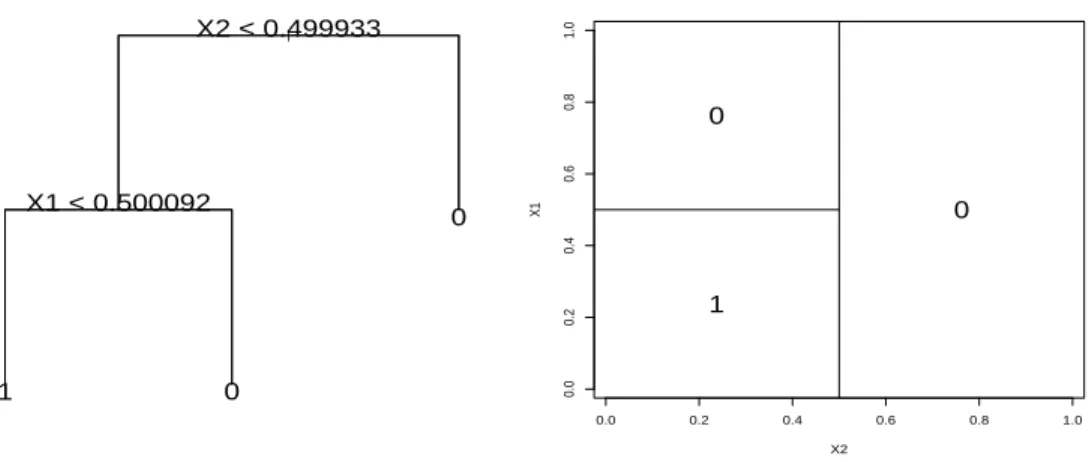
The CART algorithm provides piecewise constant classifiers represented by binary decision trees. An example of the latter is given in Figure 1 for a couple of covariates (X1, X2) belonging toX = [0; 1]2.
The tree on the left hand side of Figure 1 defines the partition of X repre-sented on the right hand side of Figure 1: each question asked on an internal node relates to a split in X. If the answer to the question is positive, go to the left child node, if not, go to the right child node. Hence the first question corresponds to a two-part partition of the covariate space. Then, each part is split into two subparts, and so on. Thus X is associated to the so calledroot of the tree, and the final partition is associated to the terminal nodes, also called leaves, of the tree. Hence each node of the tree represents a subset of the covariates space defined by the successive questions. The final partition is given by the leaves of the tree. Finally, a predictive value for the dependent variable is associated to each leaf. Thus, if Te denotes the set of leaves of a decision tree T, the classifierfT :X 7→ {0; 1}defined onTecan be written as
fT =
X
t∈Te
| X2 < 0.499933 X1 < 0.500092 1 0 0 0.0 0.2 0.4 0.6 0.8 1.0 0.0 0.2 0.4 0.6 0.8 1.0 X2 X1 1 0 0
Figure 1: Decision tree example (left) and its associated partition (right).
where at ∈ {0; 1} and 1lt(x) = 1 if x falls in the leaf t, 1lt(x) = 0 otherwise.
2.3
The CART algorithm
CART is based on a recursive partitioning using a class S of subsets of X
which determines the question to be asked at each internal node of the tree. Below, we consider general classesS with finite Vapnik-Chervonenkis dimen-sion, henceforth referred to as VC-dimension (for a complete overview of the VC-dimension see [36]). Let us notice that, theoretically, CART can be per-formed with any kind of split class S, but, in practice, the more frequently used class is that of half spaces of X with axis-parallel frontiers (which cor-responds to axis-parallel cuts) for computational reasons.
To begin with, a collection of CART classifiers is constructed by using learn-ing sample L. This collection is computed in two steps, called the growing algorithm and the pruning algorithm. The growing algorithm allows to con-struct a maximal binary tree Tmax from the data by recursive partitioning,
and then the pruning algorithm allows to select a finite collection of subtrees of Tmax.
Since our main interest in this paper is the pruning algorithm, we skip the growing algorithm (for more details about the growing algorithm, see [7]).
Just notice that the maximal treeTmax is constructed from the learning
sam-ple in such a way that, at the end of the algorithm, its leaves are pure, i.e, contain only observations having the same label.
Then, to avoid overfitting, a decision tree having good predictive perfor-mance has to be selected among all possible subtrees pruned from Tmax. Let
us recall that a pruned subtree of Tmax is defined as any binary subtree of
Tmaxhaving the same root (denotedt1) asTmax. As mentioned in [7], looking
at the whole family of subtrees pruned from Tmax is an NP-hard problem.
Then, a good alternative to the exhaustive search is the pruning algorithm, which is computed as follows.
First, let us introduce some notations:
(i) For a tree T, t is the general notation for a node of T and, if t is an internal node, Tt denotes the branch of T issued from t, that is the
subtree ofT whose root is t.
(ii) For a treeT, Te denotes the set of its leaves and |Te| the cardinality of e
T.
(iii) Take two treesT1 and T2. Then, if T1 is a pruned subtree of T2, write
T1 T2.
In the meantime, let us denote bynthe size of the sample used to pruneTmax;
in the methods detailed below, we will see that, in any case, n 6 nl < N,
where nl is the size of the learning sample L.
Second, let us notice that, given a treeT andFT the set of classifiers defined
on Teas defined by (8), the ERM classifier on FT is ˆ fT = argminf∈FTPn(f) = X t∈Te ˆ yt1lt,
where Pnis the empirical misclassification rate defined by (7), and ˆyt ∈ {0; 1}
is the majority vote inside the leaf t. Thus, if t is an internal node of T, ˆ
f|Tt denotes the restriction of ˆfT to the sub-partition associated with the
leaves of the branchTt, and Pn(t) =n−1
P
misclassification rate inside the node t.
Third, given any subtree T Tmax and α >0, one defines
critα(T) = Pn( ˆfT) +α
|Te|
n . (9)
the penalized criterion of T for the so called temperature α, and Tα the
subtree of Tmax satisfying:
(i) Tα = argminTTmaxcritα(T),
(ii) if critα(T) = critα(Tα), then Tα T.
Thus Tα is the smallest minimizing subtree for the temperature α. The
ex-istence and the unicity of Tα are proved in [7, pp 284-290].
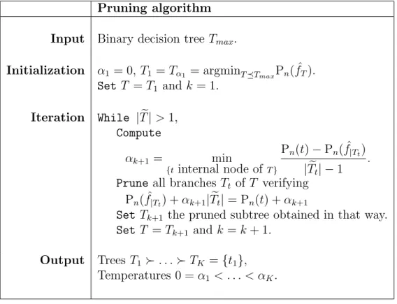
The pruning algorithm’s principle is to raise temperature α, and to record the corresponding Tα. The algorithm is summarized in Table 1 (see [7, pp
59-92] for a complete overview).
Remark 1.
1) T1 is the smallest subtree for temperature 0, so it is not necessarily equal
toTmax.
2) Tmax are T1 are constructed in such a way that, for all T T1 and all
internal node t of T, Pn(t)>Pn( ˆf|Tt); hence, αk >0 for all k >1.
3) The pruning algorithm is designed to catch, at each iteration k, the minimal temperature αk+1 for which the overall energy is kept, that is
for which critαk+1(Tk+1) = critαk+1(Tk). This property results directly
from the linearity of the penalty used in criterion (9).
Finally, the selection of a tree among the sequence (Tk)16k6K is made by
using test sample T: choose ˆk as ˆ k= argmin {16k6K} h Pnt( ˆfTk) i , (10)
where Pnt is the empirical misclassification rate onT as defined by (7). Then,
the final CART classifier is
˜
Pruning algorithm Input Binary decision tree Tmax.
Initialization α1 = 0, T1 =Tα1 = argminTTmaxPn( ˆfT).
SetT =T1 and k = 1. Iteration While |Te|>1, Compute αk+1 = min {tinternal node of T} Pn(t)−Pn( ˆf|Tt) |Tet| −1 . Prune all branches Tt of T verifying
Pn( ˆf|Tt) +αk+1|Tet|= Pn(t) +αk+1
Set Tk+1 the pruned subtree obtained in that way.
Set T =Tk+1 and k =k+ 1.
Output TreesT1 . . .TK ={t1},
Temperatures 0 =α1 < . . . < αK.
Table 1: CART pruning algorithm.
2.4
Properties of the pruned subtrees sequence
It may be easily seen that the computational complexity of the pruning algorithm is linear with respect to the number of nodes of Tmax. Hence, the
pruning algorithm is interesting in two ways:
1) It reduces drastically the computational complexity of the exhaustive search fromO(n2) to O(nlogn) (see [32] for instance),
2) It provides a small collection of trees that can be easily evaluated on T. Thus, to ensure that the CART algorithm provides good classifiers, it is important to verify that
• pruning is like looking at the entire family of pruned subtrees according to penalized criterion (9),
• pruning provides trees having good performance in term of risk condi-tionally on the growing algorithm,
• using a test sample does not alter too much the performance of the tree thus selected.
The first point has already been established by Breiman et al. [7]:
Theorem 2.4.1 (Breiman, Friedman, Olshen, Stone [7]).
For all k ∈ {1, . . . , K}, Tk = Tαk and, for all α > 0, there exists k ∈ {1, . . . , K} satisfying Tα =Tk.
Theorem 2.4.1 ensures that
1) the trees of the sequence are unique and minimize penalized criterion (9) for known temperatures,
2) whatever the choice of the temperature α used in the penalized criterion (9), Tα belongs to the sequence.
Thus, the definition of Tα leads to an infinite collection of trees over all real
α, but only finitely many trees are possible according to criterion (9).
To the best of our knowledge, the fact that the classifiers provided by CART perform well in terms of conditional risk remains to be seen. To proceed, two methods are applied to construct the sequence (Tk)16k6K. These methods,
as well as the general notations and assumptions refered to in this paper, are presented in the next section.
3
Methods, Notations and Assumptions
3.1
Methods and notations
For a given treeT,FT will denote the set of classifiers defined on the partition
given by the leaves of T, that is
FT = X t∈Te at1lt ; (at)∈ {0,1}|eT| . (11)
Thus ˆfT =
P
t∈Teyˆt1lt is the ERM classifier onFT.
The two different methods applied in the CART pruning algorithm are: M1: Lis split in two independent partsL1 andL2containing respectively
n1 and n2 observations, with n1+n2 =nl=N −nt. Hence Tmax is
constructed usingL1, then pruned usingL2. This method is applied
in Gelfandet al. [11] for instance.
M2: Tmax is constructed and pruned using sample L entirely. This is
the most commonly used method in the CART literature and its applications.
Note that a penalty is needed in both methods in order to reduce the number of candidate tree-structured models contained in Tmax. Indeed, if one does
not penalize, the number of models to be considered grows exponentially with
N (see [7]). So making a selection by using a test sample without penalizing requires visiting all the models. As mentioned above, looking for the best model in the collection of all subtrees pruned from the maximal one becomes explosive. Hence pruning allows to reduce significantly the number of trees taken into account. With both M1 and M2 methods, T is used to select a tree among the pruned sequence. Let us mention that T usually represents 10% of the data and is randomly taken in the original sample, except if the design is fixed. In that case one takes, for example, one observation out of ten to obtain the test sample. In a similar way, for the M1 method L1 and
L2 are taken randomly in L, except if the design is fixed, in which case one
takes one observation out of two for instance.
Methods M1 and M2 involve different treatments for the risks of the CART classifiers thus obtained. Indeed, by conditioning with respect to the sample used to perform the growing algorithm,Tmaxbecomes deterministic with M1,
while it implies random models depending on the sample used to pruneTmax
with M2. In the latter case, union bounds on the family of all possible trees that can be constructed on the grid {Xi ; (Xi, Yi) ∈ L} are used to obtain
risk bounds. This allows to obtain risk bounds only conditionally on this grid instead of conditionally on the grid and the labels. To simplify the notations, we define the loss and the L2 distance corresponding with either method M1
Definition 1. The loss of a classifier f is defined by λ(f∗, f), and is com-puted as follows:
(i) if f˜is constructed via M1, λ(f∗, f) := l(f∗, f), with l defined by (5). (ii) if f˜is constructed via M2, λ(f∗, f) := E[Pnl(f)−Pnl(f ∗ ) | Xi ; (Xi, Yi)∈ L] = 1 nl X {Xi ; (Xi,Yi)∈L} |2η(Xi)−1|1lf(Xi)6=f∗(Xi),
where Pnl is the empirical misclassification rate on L defined by (7), and η
is defined by (4).
Since l(f∗, f) = E|2η(X)−1|1lf(X)6=f∗(X) for all classifier f (see [9] for instance), λ is just the empirical version of l on the grid{Xi ; (Xi, Yi)∈ L}
in the M2 case.
Definition 2. The L2 distance between two classifiers f and g is defined by
d(f, g), and is computed as follows: (i) if f˜is constructed via M1, d2(f, g) := E[(f(X)−g(X))2]. (ii) if f˜is constructed via M2, d2(f, g) := d2nl(f, g) = 1 nl X {Xi ; (Xi,Yi)∈L} (f(Xi)−g(Xi))2,
As forλ,dis the empirical version of theL2distance on the grid{X
i; (Xi, Yi)∈
L} with M2.
Remark 2. If the design is fixed, λ and d are different according to the method only through the grid on which they are computed (the grid of method M1 being obtained from the one of method M2 by taking one point out of two). In this case, λ and d are no more random.
We based our computation of risk bounds for the ERM classifiers provided by CART on recent results (see for instance [21], [34], [35], [25], [17, 18], [24], [19], [16]). They stem from Vapnik’s results (see [36], [20] for example), showing that, without any assumption on the joint distribution P, the penalty term used in the penalized criterion for the model selection procedure should be taken proportional to
q
|Te|/nl to obtain classifiers optimal in term of conditional risk (see [27, 33] for instance). Nevertheless, it has also been
shown that, under the overoptimistic zero-error assumption (that is Y =
η(X) almost surely, where η is defined by (4)), this penalty term should be taken proportional to |Te|/nl, as done in criterion (9). Since we aim at
validating the choice of the penalized criterion (9) in contexts less restrictive than the zero-error one, we consider weaker assumptions on P.
3.2
Margin assumptions
Margin assumptions are now widely known to improve risk bounds of ERM classifiers in the binary classification context. One of the best-known margin assumptions is that of Mammen and Tsybakov [21] that may be written as follows:
MA(MT) There exist some constants C > 0 and κ > 1 such that, for all
t >0,
P (|2η(X)−1|6t)6C tκ−11, (12)
where η is defined by (4). MA(MT) implies the more intuitive assump-tion considered by Massart and Nedelec in [25] (see also the slightly weaker condition proposed in [16]): taking t =h ∈]0; 1[ and the limit value κ = 1,
MA(MT) leads to
MA(MN) ∃h∈]0; 1[ P (|2η(X)−1|6h) = 0.
Assumption MA(MN)means that (X, Y) is sufficiently well distributed to ensure that there is no region in X for which the toss-up strategy could be favored over others: h can be viewed as a measurement of the gap between labels 0 and 1 in the sense that, if η(x) is too close to 1/2, then choosing 0 or 1 will not make a real difference for that x.
In assumption MA(MT), η can be continuous, but has to cross the line
η(x) = 1/2 in a non smooth way.
From this simple example, the so called margin h can be viewed as a noise level for the classification problem. From this point of view, margin assump-tions have been generalized by Koltchinskii in [17]; they compare directly the loss l defined by (5) with some kind of ”noise variance” related to theL2
MA(K) There exists some strictly convex positive function ϕ satisfying
ϕ(0) = 0 such that,
∀f :X → {0; 1} l(f∗, f)>ϕpE[(f(X)−f∗(X))2]
It is easy to check that MA(MT) and MA(MN) imply MA(K) with
ϕ(x) =Cκx
2κ
2κ−1 and ϕ(x) = hx2 respectively.
Remark 3. Taking h > 1 in MA(MN) (or more generally ϕ(x) > x2 in
MA(K)) has no sense since, for any classifier f, (see [9] for instance)
l(f∗, f) = E|2η(X)−1|(f(X)−f∗(X))26E(f(X)−f∗(X))2.
MA(MT) (with κ > 1) and MA(MN) (with κ = 1) lead to risk bounds suggesting that the empirical misclassification rate of ˆfT have to be penalized
by a term proportional to|Te|/nl
κ/(2κ−1)
to obtain ERM classifiers optimal in terms of risk (see also [35] for instance), while MA(K)leads to more gen-eral penalty terms given by strictly concave functions of |Te|/nl. Hence these
margin assumptions make the link between the “global” pessimistic case (without any assumption on P) and the zero-error case by considering some noise level of the classification problem. More recent results (see [17, 18], [2] for instance) deal with data-driven penalties based on local Rademacher complexities also derived from margin assumptions.
As it can be seen in [7], the CART pruning algorithm looks at the entire family of pruned subtrees according to criterion (9) only if the penalty taken in the criterion is linear. Thus, it follows from the above mentioned results that the following margin assumption has to be fulfilled:
MA(1) ∃h∈]0; 1[ ∀f :X 7→ {0; 1} λ(f∗, f)>hd2(f∗, f),
where λ and d are defined in Definitions 1 and 2 respectively.
Examples:
1) Take X = (X1, . . . , Xd) uniformly distributed on [0; 1]d. The associated label is designed as follows: ifXj 61/2 orXj >1/2 for allj = 1, . . . , d,
2) Take X = (X1, X2) such that X1 and X2 are independently generated
with gaussian distribution N(0,1). The associated label is designed as follows: If X1 >0 and X2 >0 thenY = 1 with probability q, otherwise
Y = 1 with probability 1−q.
In these two simple examples, if q 6= 1/2, MA(MN), and consequently
MA(1), is satisfied with any value of h satisfying 0 < h < |2q−1| in both M1 and M2 cases; indeed η(X) = q orη(X) = 1−q, depending on whereX
falls. Examples in which MA(1) fails can be found in [2].
Below, we prove that, underMA(1), the penalty used by CART in criterion (9) for the pruning step leads to classifiers having good performance.
In the remaining part of this paper, the constant h will denote the so called margin.
4
Risk Bounds
This section is devoted to the results obtained on the performance of the CART classifiers for both M1 and M2 methods. These performance are re-garded from the risk viewpoint presented in paragraph 2.1, where classifiers are considered as estimators of the Bayes classifier f∗. The risk of the classi-fier ˜f provided by the CART algorithm is compared to those of the collection
ˆ
fT
TTmax
conditionally on the construction of Tmax.
We shall first present a general theorem, then give more precise results about the last two parts of the algorithm, which are the pruning algorithm and the final selection by test sample.
Theorem 1. Given N independent pairs of variables ((Xi, Yi))16i6N of
com-mon distribution P, with (Xi, Yi)∈ X × {0,1}, let us consider the estimator
˜
f (10) of the Bayes classifier f∗ (3) obtained via the CART algorithm as defined in section 2. Then we have the following results.
(i) if f˜is constructed via M1:
absolute constants C, C1 and C2 such that E h λ(f∗,f˜) | L1 i 6 C inf TTmax ( inf f∈FTE [λ(f∗, f) | L1] + |Te| hn2 ) + C1 hn2 (13) +C2 log (nl) hnt . (14) (ii) if f˜is constructed via M2:
Let PL be the L sample distribution. Let V be the Vapnik-Chervonenkis
dimension of the set of splits used to construct Tmax and suppose that nl >
V. Let K be the number of pruned subtrees of the sequence provided by the pruning algorithm, and suppose that margin assumption MA(1) is satisfied. Then, there exist some absolute constants C0, C10, C100 and C2 such that, for
every δ∈]0; 1[, on a set Ωδ verifying PL(Ωδ)≥1−δ,
E h λ(f∗,f˜) | Li 6 C0 inf TTmax ( inf f∈FT λ(f∗, f) + lognl V |Te| hnl ) + Cδ hnl (15) +C2 logK hnt , (16) with Cδ =C10 +C 00 1 log (1/δ).
Note that the constants appearing in the upper bounds for the risks are not sharp. We do not investigate the sharpness of the constants here.
Several comments can be made on the basis of the results from Theorem 1:
Methods Both methods M1 and M2 are considered for the following rea-sons:
• Since all the risks are considered conditionally on the growing pro-cedure, the M1 method permits to make a deterministic penalized model selection and then to obtain sharper upper bounds than the M2 method.
• On the other hand, the M2 method permits to keep the whole informa-tion given by L. Indeed, in that case, the sequence of pruned subtrees is not obtained via some plug-in method using a first split of the sample
to provide the collection of tree-structured models. This method is the one proposed by Breiman et al. and it is more commonly applied in practice than the former. We focus on this method to ensure that it provides classifiers that have good performance in terms of risk.
Interpretation of the bounds For both M1 and M2 methods, the in-equality of Theorem 1 may be divided into two parts:
• (13) and (15) correspond to the pruning algorithm. They show that, up to some absolute constant and the final selection, the conditional risk of the final classifier is approximately of the same order as the in-fimum of the penalized risks of the collection of subtrees of Tmax. The
term inside the infimum is of the same form as the penalized criterion (9) used in the pruning algorithm. This shows that, for a sufficiently large temperature α, this criterion allows to select convenient subtrees in term of conditional risk.
Let us emphasize that the remainder term driving the choice of the penalty is directly proportional to the number of leaves in the M1 method, whereas a multiplicative logarithmic term appears in the M2 method. This term is due to the randomness of the models consid-ered, since the samples used to construct and prune Tmax are no longer
independent.
• (14) and (16) correspond to the final selection of ˜f among the collection of pruned subtrees using T. As K 6 nl, this selection adds a term
proportional to lognl/nt for both methods, showing that not much is
lost when a test sample is used provided that nt is sufficiently large
with respect to lognl. Nevertheless, since we have no idea of the size
of the constantC2, it is difficult to deduce a general way of choosing T
from this upper bound.
Consistency results Since growing and pruning are independent when applying M1, the VC-dimension V of the set of splits S only appears with M2. Thus, in this case, the term log (nl/V) in the infimum has to be taken
into account ifV is negligeable in front ofnl. Nevertheless, if CART provides
models such that
- the approximation properties of the models are convenient enough to ensure that the bias tends to zero with increasing sample size N, then we have a result of consistency for ˜f provided that nt is conveniently
chosen with respect to lognl.
Role of the margin It has been shown in [25] and in [21] that, under mar-gin assumptionsMA(MN)andMA(MT)respectively, the ERM estimator of f∗ on one model is minimax if f∗ belongs to some H¨older classes. This means that, under margin assumptionMA(1), the upper bound obtained in Theorem 1 for the CART classifier can not be improved. On the other hand, if margin assumption MA(MT) is fulfilled, similar bounds are obtained with a remainder term in the infimum proportional to |Te|/nl
κ/(2κ−1)
. Since
κ > 1, this term is subbaditive with respect to |Te| (see [32] for full descrip-tion of subbaditive penalties), so results of [32] can be applied: the subtrees pruned by minimizing a penalized criterion with a penalty proportional to
|Te|/nl
κ/(2κ−1)
are subtrees of the CART sequence (Tk)16k6K. So, if κ is
known, the best solution is to prune Tmax with the usual pruning algorithm,
and then to extract from the sequence obtained in that way the subsequence minimizing the criterion penalized by the subadditive penalty.
Margin dependent penalties It is important to point out that the penalty term suggested by the risk bounds depends on margin parameters, which are usually unknown in practice. To withdraw the margin parameter h under margin assumption MA(1), one prunes Tmax with the pruning algorithm
given in Table 1, and then one uses a test sample or cross-validation to select a subtree. If no margin assumption is fulfilled, the procedure of Scott [32] can be applied, with a penalty term proportional to
q
|Te|/nl. Otherwise, the margin parameters have to be estimated.
Optimality of the bounds Theorem 1 also shows that the higher the margin, the smaller the risk, which is intuitive since the inverse of the margin plays the role of the classification noise. Actually, to reach opti-mality in terms of conditional risk, the penalty should be taken as cst×
h−1| e T|/nl∧ q |Te|/nl
in-fimum is, at worst, proportional to q
|Te|/nl. Hence CART will underpenalize
trees for which h6
q
|Te|/nl, leading to classifiers having an excessive num-ber of leaves. Nevertheless, the condition h >
q
|Temax|/nl can be controlled
during the growing algorithm by forcing the maximal tree’s construction to stop earlier, for example. This is obviously difficult to do in practice since it heavily depends on the data and on the size of the learning sample, and is worth being investigated more thoroughly.
The two following subsections give more precise results on the pruning algo-rithm for both the M1 and M2 methods, and particularly on the constants appearing in the penalty function. Subsection 4.2 validates the discrete se-lection by test-sample.
4.1
Validation of the Pruning algorithm
In this section, we focus more particularly on the pruning algorithm and give trajectorial risk bounds for the classifier associated with Tα, the smallest
minimizing subtree for the temperature α defined in subsection 2.3. We show that, for a convenient constant α, ˆfTα is not far from f
∗ in terms of its
conditional risk. Let us emphasize that the subsample T plays no role in the two following results.
4.1.1 f˜constructed via M1
Here we assume that L = L1 ∪ L2. Thus Tmax is constructed on the first
set of observations L1 and then pruned with the second set L2 independent
of L1. Since the set of pruned subtrees is deterministic according toL2, the
selection is made among a deterministic collection of models.
For any subtree T of Tmax, let FT be the model defined on the leaves of T
given by (11). Let Pn2 be the empirical misclassification rate onL2as defined
by (7). Then let us consider the following:
• For T Tmax, ˆfT = argminf∈FT[Pn2(f)],
• For α > 0, Tα is the smallest minimizing subtree for the temperature
Proposition 1. Let PL2 be the product distribution on L2 and let h be the
margin given by MA(1). Let ξ >0.
There exists a large enough positive constant α0 > 2 + log 2 such that, if
α > α0, then, there exist some nonnegative constants Σα and C such that
l(f∗,fˆTα) 6 C1(α) inf TTmax ( inf f∈FT l(f∗, f) +h−1|Te| n2 ) +C h−11 +ξ n2
on a set Ωξ such that PL2(Ωξ)>1−Σαe
−ξ, wherelis defined by (5), C
1(α)>
α0 and Σα are increasing with α.
We obtain a trajectorial non-asymptotic risk bound on a large probability set, leading to the conclusions given for Theorem 1. Nevertheless, taking an excessive temperature α will overpenalize and select a classifier having high riskE[l(f∗,fˆTα)| L1]. Furthermore, the fact thatC1(α) and Σαare increasing
with α suggests that both sides of the inequality grow with α. The choice of the convenient temperature is then critical to make a good compromise between the size of E[l(f∗,fˆTα) | L1] and a large enough penalty term.
4.1.2 f˜constructed via M2
Here we define the different empirical risks, expected loss and estimators exactly in the same way as in subsection 4.1.1, although l is replaced by the empirical expected loss λ onXnl
1 ={Xi ; (Xi, Yi)∈ L} defined in Definition
1. In this case, we obtain nearly the same performance for ˆfTα despite the
fact that the constant appearing in the penalty term can now depend on nl:
Proposition 2. Let PL be the product distribution on L, λ be the empirical
expected loss computed on {Xi ; (Xi, Yi)∈ L}, and let h be the margin given
by MA(1). Let ξ >0 and
αnl,V = 2 +V /2 1 + lognl V .
There exists a large enough positive constant α0 such that, if α > α0, then,
there exist some nonnegative constants Σα and C0 such that
λ(f∗,fˆTα) 6 C 0 1(α) inf TTmax ( inf f∈FT λ(f∗, f) +h−1αnl,V |Te| nl ) +C0 h−11 +ξ nl
on a set Ωξ such that PL(Ωξ)> 1−2Σαe−ξ, where C10(α) > α0 and Σα are
We obtain a similar trajectorial non-asymptotic risk bound on a large prob-ability set. The same conclusions as those derived from M1 hold in this case. Let us just mention that the remainder termh−1αnl,V|Te|/nl in the risk bound
takes into account the complexity of the collection of trees having |Te| leaves which can be constructed on {Xi ; (Xi, Yi) ∈ L}. Since this complexity
is controlled via the VC-dimension V, V necessarily appears in the penalty term. It differs from Proposition 1 in the sense that the models we consider are random, so this complexity has to be taken into account to obtain a uni-form bound.
Example: Let us consider the case where S is the set of all half-spaces of
X =Rd with axis-parallel frontiers. In this case, if d>3,
log (d)
log 2 −1.186V 6d,
consequently, if nl >d, we obtain a penalty proportional to
4 +d(1 + log [nllog 2/(logd−2 log 2)])
2h | e T| nl .
So, if CART provides some minimax estimator on a class of functions, the lognl term always appears forf∗ in this class when working in a linear space
of low dimension.
4.2
Final Selection
We focus here on the selection of the classifier ˜famong the collection ( ˆfTk)16k6K
provided by the pruning algorithm as defined in subsection 2.3. Let us recall that ˜f is defined by ˜ f = argmin {fˆ Tk;16k6K} h Pnt( ˆfTk) i ,
where Pnt is the empirical misclassification rate on T defined by (7).
The performance of this classifier can be compared to the performance of the collection ( ˆfTk)16k6K by the following:
Proposition 3.
exist three absolute constants C00 >1, C10 >3/2 and C20 >3/2 such that E h λ(f∗,f˜) | Li 6 C00 inf 16k6Kλ(f ∗ ,fˆTk) +C 0 1 h −1logK nt +h−1C 0 2 nt ,
where K is the number of pruned subtrees extracted during the pruning algo-rithm.
5
Concluding Remarks
We have proven that CART provides convenient classifiers in terms of con-ditional risk under the margin assumption MA(1). As for the regression case, the properties of the growing algorithm need to be analyzed to obtain full unconditional upper bounds. Results on the performance of theoretical procedures in which CART is viewed as a forward algorithm to approximate an ideal, but intractable, binary tree are given in [13]. Although they do not validate any concrete algorithm as done here, these results confirm that the penalty term used in penalized criterion (9) is well chosen underMA(1). The remarks made after Theorem 1 on the size of the margin h enlarge our perspectives for the application of CART in practice. Among such perspec-tive, we may
• use the slope heuristic (see for example [3]) to select a classifier among a collection,
• search for a robust manner to determine if the margin assumption is fulfilled, allowing to use the blind selection by test sample.
Some track to estimate the margin h if assumptionMA(1) is fulfilled could be to use mixing procedures as boosting (see [6] [10] for example). Hence, this estimate could be used in the penalized criterion to help find the conve-nient temperature. It could also give an idea of the difficulty to classify the considered data and henceforth to help choose the most adapted classification method.
Acknowledgements
I would like to thank an anonymous referee for numerous remarks and sug-gestions which helped to improve the presentation of this paper.
6
Proofs
Let us start with a preliminary result.
6.1
Local Bound for Tree-Structured Classifiers
Let (X, Y)∈ X ×{0; 1}be a pair of random variables and{(X1, Y1), . . . ,(Xn, Yn)}
be n independent copies of (X, Y). Then given two classifiers f andg, let us define d2n(f, g) = 1 n n X i=1 (f(Xi)−g(Xi))2. Let M∗
n be the set of all possible tree-structured partitions that can be
constructed on the grid Xn
1, corresponding to trees having all possible splits
in S and all possible forms without taking account of the response variable
Y. So M∗
n only depends on the grid X1n and is independent of the variables
(Y1, . . . , Yn). Hence, for a tree T ∈ M∗n, define
FT = X t∈Te at1lt ; (at)∈ {0,1}|eT| ,
where Te refers the set of the leaves of T. Then, for any f ∈ FT and any
σ > 0, define
BT(f, σ) = {g ∈ FT ; dn(f, g)6σ}
For each classifier f : X → {0,1}, let us define the empirical contrast of f
recentered conditionally on Xn
1
Pn(f) = Pn(f)−E[Pn(f)| X1n], (17)
where Pn is defined for any given classifier f by
Pn(f) = 1 n n X i=1 1lf(Xi)6=Yi.
Remark 4. If Pn is evaluated on a sample (Xi0) independent of X1n, it is
easy to check that the bounds we obtain in what follows are still valid by taking the population distance
instead of its empirical version dn.
We have the following result:
Lemma 1. For any f ∈ FT and any σ >0
E " sup g∈BT(f,σ) |Pn(g)−Pn(f)| | X1n # 62 σ s |Te| n .
Proof. First of all, let us mention that, since the different variables we con-sider take values in {0; 1}, we have for all x∈ X and ally ∈ {0,1}
1lg(x)6=y−1lf(x)6=y = (g(x)−f(x))(1−21ly=1), yielding Pn(g)−Pn(f) = 1 n n X i=1 (g(Xi)−f(Xi)) (1−21lYi=1) −E " 1 n n X i=1 (g(Xi)−f(Xi)) (1−21lYi=1) | X n 1 # .
Let us now consider a Rademacher sequence of random signs (εi)16i6n
inde-pendent of (Xi, Yi)16i6n. Then, one has by a symmetrization argument
E " sup g∈BT(f,σ) |Pn(g)−Pn(f)| | X1n # 6E " sup g∈BT(f,σ) 2 n n X i=1 εi(g(Xi)−f(Xi))(1−21lYi=1) | X1n # .
Since g and f belong toFT, we have that
g−f =X
t∈Te
(at−bt)ϕt,
where each (at, bt) takes values in [0,1]2 and (ϕt)t∈Te is an orthonormal basis
of FT adapted to Te (i.e some normalized characteristic functions). Then, by applying the Cauchy-Schwarz inequality, since g ∈ BT(f, σ), d2n(f, g) =
P t∈Te(at−bt) 2 6σ2, we obtain that n X i=1 εi(g(Xi)−f(Xi))(1−21lYi=1) 6 s X t∈Te (at−bt)2 v u u u t X t∈Te n X i=1 εi(1−21lYi=1)ϕt(Xi) !2 6 σ v u u u t X t∈Te n X i=1 εi(1−21lYi=1)ϕt(Xi) !2 .
Finally, since (εi)16i6n and (1− 21lYi=1)16i6n take their values in {−1; 1},
(εi)16i6n are centered and independent of (Xi, Yi)16i6n, and since, by
defini-tion, for each t∈T ne −1 Pn
i=1ϕ 2
t(Xi) = 1, Jensen’s inequality implies
E " sup g∈BT(f,σ) |Pn(g)−Pn(f)| | X1n # 62σ n v u u t X t∈Te n X i=1 ϕ2 t(Xi)62σ s |Te| n .
6.2
Proof of Proposition 1
To prove Proposition 1, we adapt results from Massart [23, Theorem 4.2], and Massart and N´ed´elec [25] (see also Massart et.al. [24]).
Let n = n2. Let us give a sample L2 = {(X1, Y1), . . . ,(Xn, Yn)} of the
random variable (X, Y) ∈ X ×[0,1], where X is a measurable space and let f∗ ∈ F ⊂ {f : X 7→ [0,1] ; f ∈ L2(X)} be the unknown function
to be recovered. Assume (Fm)m∈Mn is a countable collection of countable
models included in F. Let us give a penalty function penn : Mn −→ R+,
and γ : F ×(X ×[0,1]) −→ R+ a contrast function, i.e. γ such that f 7→
E[γ(f,(X, Y))] is convex and minimum at point f∗. Hence define for all
f ∈ F the expected loss l(f∗, f) =E[γ(f,(X, Y))−γ(f∗,(X, Y))]. Finally let γn= 1 n n X i=1 γ(.,(Xi, Yi)) (18)
be the empirical contrast associated withγ. For example, in the classification context, γ(f,(x, y)) = 1lf(x)6=y, leading to the classical loss as defined by (5),
and the classical empirical misclassification rate Pnas defined by (7). Hence,
if the collection of models Mn has finite-dimensional models with dimension
|m|, the penalty function can be taken as penn(m) =cst × |m| for instance. Then let ˆm be defined as
ˆ m= argmin m∈Mn h γn( ˆfm) + penn(m) i
where ˆfm = argming∈Fmγn(g) is the minimum empirical contrast estimator
of f∗ onFm. The final estimator of f∗ is
˜
One makes the following assumptions:
H1: γ is bounded by 1, which is not a restriction since all the functions we
consider take values in [0,1].
H2: Assume there exist c > (2
√
2)−1/2 and some (pseudo-)distance d such
that, for every pair (f, g)∈ F2, one has
Var [γ(g,(X, Y))−γ(f,(X, Y))]6d2(g, f),
and particularly for all f ∈ F
d2(f∗, f)6c2l(f∗, f).
H3: For any positive σ and for any f ∈ Fm, let us define
Bm(f, σ) ={g ∈ Fm ; d(f, g)6σ}
where d is given by assumption H2. Let ¯γn = γn(.)− E[γn(.)]. We now
assume that for any m ∈ Mn, there exists some continuous function φm
mapping R+ ontoR+ such thatφm(0) = 0,φm(x)/x is non-increasing and
E " sup g∈Bm(f,σ) |¯γn(g)−γ¯n(f)| # 6φm(σ)
for every positive σ such that φm(σ)6σ2. Let εm be the unique solution of
the equation φm(cx) =x2 , x >0.
One gets the following result:
Theorem 2. Let {(X1, Y1), . . . ,(Xn, Yn)} be a sample of independent
real-izations of the random pair (X, Y)∈ X ×[0,1]. Let (Fm)m∈Mn be a
count-able collection of models included in some countcount-able family F ⊂ {f : X 7→
[0,1] ; f ∈L2(X)}. Consider some penalty function pen
n:Mn −→R+ and
the corresponding penalized estimator f˜(19) of the target function f∗. Take a family of weights (xm)m∈Mn such that
Σ = X
m∈Mn
e−xm <+∞. (20)
Assume that assumptions H1, H2 and H3 hold.
Let ξ > 0. Hence, given some absolute constant C > 1, there exist some positive constants K1 and K2 such that, if for all m∈ Mn
penn(m)>K1ε2m+K2c2
xm
then, with probability larger than 1−Σe−ξ, l(f∗,f˜)6C inf m∈Mn [l(f∗,Fm) + penn(m)] +C 0 c21 +ξ n , where l(f∗,Fm) = inffm∈Fml(f ∗, f
m)and the constant C0 only depends on C.
Proof. The proof is inspired from Massart [23] and Massart et.al. [24]. We give only sketches of proofs since those are now routine results in the model selection area (see [24] for a fuller overview).
Let m∈ Mn and fm ∈ Fm. The definition of the expected loss and the fact
that
γn( ˜f) + penn( ˆm)6γn(fm) + penn(m)
lead to the following inequality:
l(f∗,f˜)6l(f∗, fm) + ¯γn(fm)−¯γn( ˜f) + penn(m)−penn( ˆm) (21)
where ¯γn is defined by (17). The general principle is now to concentrate
¯
γn(fm)−γ¯n( ˜f) around its expectation in order to offset the term penn( ˆm).
Since ˆm ∈ Mn, we proceed by bounding ¯γn(fm)− γ¯n( ˆfm0) uniformly in
m0 ∈ Mn. For m0 ∈ Mn and f ∈ Fm0, let us define
wm0(f) = hp l(f∗, f m) + p l(f∗, f)i2 +y2 m0,
with ym0 >εm0, whereεm0 is defined by assumptionH3. Hence let us define
Vm0 = sup f∈Fm0 ¯ γn(fm)−γ¯n(f) wm0(f) . Then (21) becomes l(f∗,f˜) 6 l(f∗, fm) +Vmˆwmˆ( ˜f) + penn(m)−penn( ˆm)
Since Vm0 can be written as
Vm0 = sup f∈Fm0 νn γ(fm, .)−γ(f, .) wm0(f) ,
whereνnis the recentered empirical measure, we boundVm0 uniformly inm0 ∈
be found in [29], and recalled here: if F is a countable family of measurable functions such that, for some positive constantsv andb, one has for allf ∈ F
P(f2)6v and kfk∞6 b, then for every positive y, the following inequality
holds for Z = supf∈F(Pn−P)(f)
P " Z−E(Z)> r 2(v + 4bE(Z))y n + by n # 6e−y.
To proceed, we need to check the two bounding assumptions. First, since by assumption H1 the contrast γ is bounded by 1, we have that, for each
f ∈ Fm0, γ(f, .)−γ(fm, .) wm0(f) 6 1 y2 m0 . (22)
Second, by using assumption H2, we have that, for each f ∈ Fm0,
Var γ(f,(X, Y))−γ(fm,(X, Y)) wm0(f) 6 c 2 4y2 m0 . (23)
Then, by Rio’s inequality, we have for every x >0
P " Vm0 >E(Vm0) + s c2+ 16 E(Vm0) 2nym20 x+ x nym20 # 6e−x.
Let us takex=xm0+ξ,ξ >0, wherexm0 is given by (20). Then, by summing up over m0 ∈ Mn, we obtain that for allm0 ∈ Mn
Vm0 6E(Vm0) + s c2+ 16 E(Vm0) 2ny2 m0 (xm0+ξ) + xm0 +ξ ny2 m0
on a set Ωξ such that P(Ωξ) > 1−Σe−ξ. We now need to bound E(Vm0) in order to obtain an upper bound for Vm0 on the set of large probability Ωξ. By using techniques similar to Massart et al.’s [25], we obtain the
fol-lowing inequality via the monoticity of x 7→ φ(x)/x and the assumption
c>(2√2)−1/2: for allm0 ∈ Mn, let um0 ∈ Fm0 be defined by
l(f∗, um0)62 inf z∈Fm0
Then we have E(Vm0)6E " sup z∈Fm0 |γ¯n(z)−γ¯n(um0)| wm0(z) # +E |¯γn(um0)−¯γn(fm)| infz∈Fm0[wm0(z)] .
For every z ∈ Fm0, let
ω2m0(z) = l(f∗, um0) +E[γ(z,(X, Y))−γ(um0,(X, Y))] +. Then, since l(f∗, z) = E[γ(z,(X, Y))−γ(f∗,(X, Y))] l(f∗, z) = l(f∗, um0) +E[γ(z,(X, Y))−γ(um0,(X, Y))], Then we have l(f∗, z)6ωm20(z)65l(f∗, z). (24) On the one hand we have wm0(z) > l(f∗, z) +y2
m0 > (1/5)ω2m0(z) + ym20 for every z ∈ Fm0. Hence E " sup z∈Fm0 |γ¯n(z)−γ¯n(um0)| wm0(z) # 65 E " sup z∈Fm0 |¯γn(z)−¯γn(um0)| ω2 m0(z) + 5y2m0 # . Furthermore we have E " sup {z ;ωm0(z)6ε} |γn(z)−γn(um0)| # 6E " sup {z ; l(f∗,z)6ε2} |γn(z)−γn(um0)| # , and, if l(f∗, z) 6 ε2, then l(f∗, u m0) 6 2ε2 and d(z, um0) 6 d(f∗, z) + d(s∗, um0)6cε+cε √
2. Hence we get that d(z, um0)6(1 +
√
2)cε62cε√2. Let us now suppose thatε>εm0. Then we have by monoticity ofx7→φ(x)/x and by definition of εm0 that
φm0(2cε √ 2) (2cε√2)2 6 φm0(cε) c2ε22√2 6 φm0(cεm0) c2ε2 m02 √ 2 61 since c>(2√2)−1/2.
So, by assumption H3, we finally obtain that, for allε>εm0, E " sup {z ; ωm0(z)6ε} |γn(z)−γn(um0)| # 6E " sup {z ;d(z,u 0)62cε√2} |γn(z)−γn(um0)| # 6φm0(2cε √ 2).
So we can apply Lemma 5.5 in [25] and use the monoticity of x7→φm0(x)/x to obtain that E " sup z∈Fm0 |¯γn(z)−¯γn(um0)| wm0(z) # 64φm0(2c √ 10ym0) y2 m0 68√10 φm0(cym0) y2 m0 .
Hence, since ym0 > εm0 and x 7→ φm0(cx)/x is nonincreasing, we get by definition of εm0 E " sup z∈Fm0 |γ¯n(z)−γ¯n(um0)| wm0(z) # 68√10φm0(cεm0) ym0εm0 6 8√10εm0 ym0 .
On the other hand, let us notice that inf z∈Fm0 wm0(z) > 2ym0 inf z∈FSm0 [pl(f∗, z) +pl(f∗, f m)] > ym0 √ 2 c d(um0, fm), hence E |γ¯n(um0)−γ¯n(fm)| infz∈Fm0[wm0(z)] 6c(ym0 √ 2)−1E |γ¯n(um0)−γ¯n(fm)| d(um0, fm) ,
leading by Jensen’s inequality to E |¯γn(um0)−¯γn(fm)| infz∈Fm0[wm0(z)] 6c(ym0 √ 2)−1 p Var [¯γn(um0)−γ¯n(fm)] d(um0, fm) 6 c ym0 √ 2n.
Then we get for all m0 ∈ Mn
E[Vm0]6 8√10εm0 +c(2n)−1/2 ym0 . Hence, taking ym0 =K " 8√10εm0 +c(2n)−1/2+c r xm0+ξ n #
with K >0, we obtain that, on Ωξ, for all m0 ∈ Mn,
Vm0 6 1 K " 1 + s 1 2 1 + 8 K√2 + 1 2K√2 # .
So we finally obtain that, on the set Ωξ, l(f∗,f˜)6l(f∗, fm) +K0wmˆ( ˜f) + penn(m)−penn( ˆm), (25) with K0 = 1 K " 1 + s 1 2 1 + 8 K√2 + 1 2K√2 # .
Finally, by using repeatedly the elementary inequality (α+β)2 62α2+ 2β2
to bound y2 ˆ
m and wmˆ( ˜f), we derive that, on the one hand,
y2mˆ 64K2 640ε2mˆ + c 2 2n +c 2 xmˆ +ξ 2n ,
and, on the other hand,
wmˆ( ˜f)62l(f∗,f˜) + 2l(f∗, fm) +y2mˆ.
Hence the following inequality holds on Ωξ for any m ∈ Mn and any fm ∈
Fm: (1−2K0 )l(f∗,f˜) 6 (1 + 2K0)l(f∗, fm) + penn(m) + 2K 0K2ξ n + 2c2K0K2 n +5×29K0K2εm2ˆ + 2c2K0K2xmˆ n −penn( ˆm), with K0 = C−1 2(C+ 1), K1 = 5×2 9 K0K2, K2 = 2K0K2.
Application to classification trees:
Let us now suppose that (X, Y) takes values inX × {0,1}. The contrast is taken as γ(f,(X, Y)) = 1lf(X)6=Y, the expected loss is defined by (5), and
the collection of models is (FT)TTmax. The models and the collection are
countable since there is a finite number of functions in each FT, and a finite
number of nodes in Tmax. Since we are working conditionally on L1, we can
apply Theorem 2 directly with L2. To check assumption H2, let us first note
that, since all the variables we consider take values in {0,1}, we have the following for all classifiers f and g
(γ(f,(X, Y))−γ(g,(X, Y)))2 = 1lY6=f(X)−1lY6=g(X)
2
(26) = (f(X)−g(X))2. (27)
Then, if we taked2(f, g) =
E[(f(X)−g(X))2], we have that, for all classifiers
f and g, Var [γ(g,(X, Y))−γ(f,(X, Y))] 6 d2(f, g). Moreover, with the margin condition MA(1), we have that
l(f∗, f) > hd2(f∗, f), (28) hence assumptionH2 is checked withdand c2 = 1/h, wherehis the margin.
By definition of h, we have h6162√2, and then c>(2√2)−1/2.
Then, assumption H3 is checked by Lemma 1 with φT(x) = 2x
q
|Te|/n. Hence, Theorem 2 is verified with εT =
p 1/h
q
|Te|/n.
Finally, to choose a convenient family of weights (xT)TTmax, taking xT =
θ|Te|, with θ > 2 log 2 independent of |Te| as done in [14], we immediately obtain Σα= Σθ <+∞. Then, we get proposition 1 by Theorem 2.
6.3
Proof of Proposition 2
Let n=nl and letX1n denote the sample{Xi ; (Xi, Yi)∈ L}.
First we generalize Theorem 2 to random models, and then we apply it to CART. Let (X, Y), F, f∗ ∈ F, L = {(X1, Y1), . . . ,(Xn, Yn)}, γ and γn be
defined as in subsection 6.2. Finally, let us rewrite the expected loss off ∈ F
conditionally on Xn
1 as in Definition 1, that is
λ(f∗, f) =E[Pnl(f)−Pnl(f
∗
) | X1n].
Let us consider a collection of at most countable models (Fm)m∈M∗
n and a
sub-collection (Fm)m∈Mn, whereMn⊂ M
∗
nmay depend on{(X1, Y1), . . . ,(Xn, Yn)}.
Finally, let us consider a penalty function penn:Mn 7→R+and let us define
the estimator ˜f of f∗ as follows: let ˆ
m= argminm∈Mn[γn( ˆfm) + penn(m)],
where ˆfm = argminf∈Fmγn(f) is the minimum contrast estimator of f
∗ on
Fm. Then ˜f = ˆfmˆ.
Let us make the following assumptions.
H1: γ is bounded by 1.
H2: Assume there exist c>(2
√
2)−1/2 and some (pseudo-)distance d
n (that
may depend on Xn
1) such that, for every pair (g, f)∈ F2, one has
and particularly for all f ∈ F
d2n(f∗, f)6c2λ(f∗, f).
H3: For any positive σ and for any f ∈ Fm, let us define
Bm(f, σ) ={g ∈ Fm ; dn(f, g)6σ}
where dn is given by assumption H2. Let ¯γn be defined as (17). We now
assume that for any m ∈ Mn, there exists some continuous function φm
mapping R+ ontoR+ such thatφm(0) = 0,φm(x)/x is non-increasing and
E " sup g∈Bm(f,σ) |γ¯n(g)−γ¯n(f)| | X1n # 6φm(σ)
for every positive σ such that φm(σ)6σ2. Let εm be the unique solution of
the equation φm(cx) =x2 , x >0.
One gets the following result.
Theorem 3. Let L = {(X1, Y1), . . . ,(Xn, Yn)} be a sample of independent
realizations of the random pair (X, Y) ∈ X ×[0,1]. Let (Fm)m∈M∗
n be a
countable collection of models included in some countable family F ⊂ {f :
X 7→ [0,1] ; f ∈L2(X)}(which may depend on Xn
1). Consider some
subcol-lection of models (Fm)m∈Mn, where Mn⊂ M
∗
n may depend on L, and some
penalty function penn: Mn −→R+. Let f˜(19) be the corresponding
penal-ized estimator of the target function f∗. Take a family of weights (xm)m∈M∗
n such that X m∈M∗ n e−xm 6Σ<+∞, (29)
with Σ deterministic. Assume that assumptions H1, H2 and H3 hold.
Let ξ > 0. Hence, given some absolute constant C > 1, there exist some positive constants K1 and K2 such that, if for all m∈ Mn
penn(m)>K1ε2m+K2c2
xm
n ,
then, with probability larger than 1−2Σe−ξ,
λ(f∗,f˜)6C inf m∈Mn [λ(f∗,Fm) + penn(m)] +C 0 c21 +ξ n , where λ(f∗,Fm) = inffm∈Fmλ(f ∗, f
m) and the constant C0 only depends on
Proof. The proof is highly similar to that of Theorem 2. The main differences are in the conditioning and the fact that the collection of models (Fm)m∈Mn
is random. To remove these issues, all the bounds are computed uniformly on M∗
n so that the probability of the set we finally obtain is unconditional
to Xn
1 since Σ is deterministic. The inequalities are obtained by the same
techniques as the ones used for the proof of the results on model selection on random models done by Gey and N´ed´elec in [14].
Let m∈ Mn and fm ∈ Fm. Starting from (21), we have
λ(f∗,f˜) 6 λ(f∗, fm) +wm,mˆ ( ˜f)Vm,mˆ + penn(m)−penn( ˆm), (30)
where for all m0 and M in M∗
n, for all f ∈ Fm0 and fM ∈ FM,
wm0,M(f) = hp l(f∗, f) +pλ(f∗, f M) i2 + (ym0 +yM)2, Vm0,M = sup f∈Fm0 ¯ γn(fM)−¯γn(f) wm0,M(f) ,
with ym0 >εm0 and yM >εM. The general principle is now exactly the same as in the proof of Theorem 2 despite the fact that we have to bound Vm0,M not only uniformly in m0 ∈ M∗
n, but also in M ∈ M
∗
n in order to have an
in-probability inequality that does not depend on X1n.
Assumption H2 allows to give exactly the same upper bounds (except that
they depend on Xn
1 and that ym0 is replaced byym0 +yM) as (22) and (23). By using the same techniques as in the proof of Theorem 2 and the same considerations as in [14], we obtain that
E[Vm0,M | Xn 1]68 √ 10φm0(cym0 +cyM) (ym0 +yM)2 + c (ym0 +yM) √ 2n.
Then, since ym0 +yM >ym0 >εm0 and εM >0, we get by definition of εm0 8√10φm0(cym0+cyM) (ym0 +yM)2 6 8√10 φ(cεm0) (ym0+yM)εm0 6 8√10εm0 +εM ym0 +yM . So we have E[Vm0,M | X1n]6 8√10(εm0 +εM) +c(2n)−1/2 ym0 +yM .
Summing up over m0 ∈ M∗
n and M ∈ M
∗
n, that leads by Rio’s inequality, to
Vm0,M 6 1 ym0 +yM 8√10εm0 + c(2n)−1/2 2 + 8 √ 10εM + c(2n)−1/2 2 + s c2+ 16(8√10(ε m0 +εM) +c(2n)−1/2)(ym0 +yM)−1 2n(y2 m0 +y2M) (xm0+xM +ξ) + 1 y2 m0+y2M xm0 +ξ/2 n + xM +ξ/2 n
on a set Ωξsuch thatP (Ωξ | X1n)>1−2Σe
−ξ. Then, since Σ is deterministic,
we get that P(Ωξ)>1−2Σe−ξ.
Hence, if we take for all m0 ∈ M∗
n ym0 = 2K " 8√10εm0 + c(2n)−1/2 2 +c r xm0 +ξ/2 n # ,
we obtain that, on Ωξ, for allm0 and M inM∗n,
Vm0,M 6 1 K " 1 + s 1 2 1 + 8 K√2 + 1 2K√2 # .
Finally the proof is achieved in the same way as the proof of Theorem 2. Application to classification trees:
Let us consider the classification framework and the collection of models (FT)TTmax obtained via the growing algorithm in CART (see subsection 4.1)
as recalled in subsection 6.2. Since the growing and the pruning algorithms are made on the same sample L, the conditions of Theorem 3 hold. Since
n = nl is fixed, let us consider M∗n as the set of all possible tree-structured
partitions that can be constructed on the grid Xn
1, corresponding to trees
having all possible splits in S and all possible forms without taking account of the response variable Y. So M∗
n depends only on the grid X1n and is
independent of the variables (Y1, . . . , Yn). Then {T Tmax} ⊂ M∗n and we
are able to apply Theorem 3. Considering (26), we take
d2n(f, g) = 1 n n X i=1 (f(Xi)−g(Xi))2,
corresponding with the distance d given in Definition 2. Using the margin condition MA(1), (28) is also verified forλ anddn, and we have assumption
H2 with c2 = 1/h. Then, by Lemma 1, assumption H3 is checked with
φT(x) = 2x
q
|Te|/n and, in the same way as in the proof of Proposition 1,
εT is taken as εT =
p 1/h
q
|Te|/n.
Finally, to choose a convenient family of weights (xT)T∈M∗
n, taking (see [14]) xT =V θ+ logn1 V |Te|,
where V is the VC-dimension of the set of splits S used to construct Tmax
and θ > 1, we obtain
Σα= Σθ =
X
D>1
exp (−(θ−1)DV)<+∞.
And we have Proposition 2.
6.4
Proof of Proposition 3
Proposition 3 is a direct application of the theorem obtained by Blanchard and Massart in [18], reformulated for our purpose here: assume that we observe N +n independent random variables with common distribution P
depending on a parameter f∗ to be estimated. Suppose the first N obser-vations Z0 = Z10, . . . , ZN0 are used to build some preliminary collection of estimators ( ˆfm)m∈Mn and the remaining observations Z1, . . . , Zn are used to
select an estimator ˜f among this collection by minimizing the empirical con-trast as defined by (18) (with (X, Y) replaced by Z). Hence, we have the following result.
Theorem 6.4.1 (Blanchard and Massart [18]).
Suppose that Mn is finite with cardinal K. Assume that there exists some
continuous function w mapping R+ onto R+ such that x 7→ w(x)/x is
non-increasing, and which satisfies for all ε >0 sup
{f∈F ; l(f∗,f)6ε2}
Var [γ(f, Z)−γ(f∗, Z)]6w(ε). (31)
Then one has for every θ ∈(0,1)
(1−θ)Ehl(f∗,f˜) | Z0i 6(1+θ) inf m∈Mn l(f∗,fˆm)+δ2∗ 2θ+ (1 + log (K))(1 3+ 1 θ) ,
where l is defined by (5) and δ∗ satisfies
√
nδ2
∗ =w(δ∗).
Taking w(ε) = (1/√h)ε for both methods M1 and M2, where h is the margin, leads to proposition 3 with
C = 1 +θ 1−θ, C1 = θ+ 3 2θ(1−θ), C2 =C1+ θ 1−θ.
6.5
Proof of Theorem 1
We are now able to prove Theorem 1 via propositions 1, 2 and 3. The beginning of the proof remains the same if ˜f is constructed either via M1 or M2. So we just give the first step of the proof for the M1 method.
Actually, since we have at most one model per dimension in the pruned subtree sequence, it suffices to note thatK 6n1. Then letα0 be the minimal
constant given by Proposition 1. Hence, since for a given α >0 Tα belongs
to the sequence (Tk)16k6K, E h l(f∗,f˜) | L1, L2 i 6C00 inf α>α0 l(f∗,fˆTα) +C 0 1 h −1logK nt +h−1C 0 2 nt .
Starting from this inequality, if ˜f is constructed via M1, by using Proposition 1 with α = 2α0 and by taking the expectation according to L2, we obtain
Theorem 1 with the appropriate constants.
Yet, if ˜f is constructed via M2, we apply Proposition 2 with α = 2α0αn1,V
and, for each δ ∈]0; 1[, ξ = log (2Σα/δ). Then, we obtain Theorem 1 with
the appropriate constants.
References
[1] A¨ızerman, M. A., Braverman, E. M., and Rozono`er, L. I.
Method of Potential Functions in the Theory of Learning Machines. Nauka, Moscow (in Russian). 1970.
[2] Arlot, S., and Bartlett, P. Margin adaptive model selection in
statistical learning. Tech. Rep. 0804.2937, arXiv, 2008.
[3] Arlot, S., and Massart, P. Data-driven calibration of penalties
for least-squares regression. Journal of Machine Learning Research 10 (2009), 245–279.
[4] Blanchard, G., Schafer, C., Rozenholc, Y., and Muller, K.-R. Optimal dyadic decision trees. Machine Learning 66, 2-3 (2007),
209–242.
[5] Boucheron, S., Bousquet, O., and Lugosi, G. Theory of
clas-sification: a survey of some recent advances. ESAIM Probab. Stat. 9 (2005), 323–375 (electronic).
[6] Breiman, L. Arcing classifiers. Ann. Statist. 26, 3 (1998), 801–849.
With discussion and a rejoinder by the author.
[7] Breiman, L., Friedman, J. H., Olshen, R. A., and Stone, C. J. Classification And Regression Trees. Chapman & Hall, 1984.
[8] Chou, P. A., Lookabaugh, T., and Gray, R. M. Optimal pruning
with applications to tree-stuctured source coding and modeling. IEEE Transactions on Information Theory 35, 2 (1989), 299–315.
[9] Devroye, L., Gy¨orfi, L., and Lugosi, G. A probabilistic theory of
pattern recognition, vol. 31 ofApplications of Mathematics (New York). Springer-Verlag, New York, 1996.
[10] Freund, Y., and Schapire, R. E.A decision-theoretic generalization
of on-line learning and an application to boosting. Journal of Computer and System Sciences 55, 1 (1997), 119–139.
[11] Gelfand, S. B., Ravishankar, C., and Delp, E. J. An itera-tive growing and pruning algorithm for classification tree design. IEEE Transactions on PAMI 13, 2 (1991), 163–174.
[12] Gey, S., and Lebarbier, E. Using cart to detect multiple change-points in the mean for large samples. Tech. Rep. 12, SSB, 2008.
[13] Gey, S., and Mary Huard, T. Risk bounds for embedded variable
selection in classification trees. Tech. rep., arxiv, 1108.0757v1, 2011. [14] Gey, S., and Nedelec, E. Model selection for CART regression trees.
IEEE Trans. Inform. Theory 51, 2 (2005), 658–670.
[15] Hastie, T., Tibshirani, R., and Friedman, J. The elements of statistical learning. Springer, 2001.