Individualized learning and integration for multi-modality data

(1)

c

(2)

INDIVIDUALIZED LEARNING AND INTEGRATION FOR MULTI-MODALITY DATA

BY

Xiwei Tang Dissertation XIWEI TANG

DISSERTATION Xiwei Tang Dissertation

Submitted in partial fulfillment of the requirements for the degree of Doctor of Philosophy in Statistics

in the Graduate College of the

University of Illinois at Urbana-Champaign, 2017

Urbana, Illinois

Doctoral Committee: Xiwei Tang Dissertation

Professor Annie Qu, Chair Professor Xiaofeng Shao Professor Douglas Simpson Assistant Professor Ruoqing Zhu Xiwei Tang Dissertation

(3)

Abstract

Individualized modeling and multi-modality data integration have experienced an explosive growth in recent years, which have many important applications in biomedical research, personalized ed-ucation and marketing. Conventional statistical models usually fail to capture significant variation due to subject-specific effects and heterogeneity of data from multiple sources. Consequently, it has become very critical to incorporate individuals’ and modalities’ heterogeneous characteristics in order to efficiently explore the data structure and enhance the prediction power. In this thesis, we address three challenging issues: mixture modeling for longitudinal data, individualized variable selection and multi-modality tensor learning with an application in medical imaging analysis.

In the first part of the thesis, we develop a model-based subgrouping method for longitudinal data. Specifically, we propose an unbiased estimating equation approach for a two-component mix-ture model with correlated response data. In contrast to most existing longitudinal data clustering methods, the proposed model allows subgroup membership change for each individual over time. Furthermore, we incorporate correlation structure on unobservable latent indicator variables. An-other advantage our approach is that we do not require any information about joint likelihood func-tion for each subject. The proposed model is shown to have more efficient parameter estimators in both mixing proportions and component densities. In addition, by utilizing within-subject serial correlations, the proposed approach enhances classification power compared to existing methods, especially for those boundary observations.

In the second part of the thesis, we propose an individualized variable selection approach to select different relevant variables for different individuals. The conventional homogeneous model, which assumes all subjects share the same effects of certain predictors, may wash out important information due to heterogeneous variation. For example, in personalized medicine, some indi-viduals could have positive responses to the treatment while some indiindi-viduals could have negative ones. Hence the population average effect could be close to zero. In this thesis, we construct a

(4)

separation penalty with multi-directional shrinkages including zero, which facilitates individual-ized modeling to distinguish strong signals from noisy ones. As a byproduct, the proposed model identifies subgroups among which individuals share similar effects, and thus improves estimation efficiency and personalized prediction accuracy. Finite sample simulation studies and an applica-tion to HIV longitudinal data demonstrate the model efficiency and the predicapplica-tion power of the new approach compared to a variety of existing penalization models.

In the third part of the thesis, we are interested in employing medical imaging data for diag-nosis. This work is motivated by breast cancer imaging data produced by a multimodality multi-photon optical imaging technique. We develop an innovative multilayer tensor learning method to predict disease status effectively through utilizing subject-wise imaging information. In particular, we propose an individualized multilayer model which leverages an additional layer of individual structure of imaging shared by multiple modalities in addition to employing a high-order tensor decomposition shared by populations. One major advantage of our approach is that we are able to capture the spatial information of microvesicles observed in certain modalities of optical imaging through integrating multimodality imaging data. Our simulation studies and real data analysis both indicate that the proposed multilayer learning method improves prediction accuracy significantly compared to existing competitive statistical and machine learning methods.

(5)

(6)

Acknowledgements

First and foremost, I would like to express my sincerest gratitude to my advisor Professor Annie Qu for her guidance on all the aspects of my Ph.D life. Her patience, enthusiasm, passion and immense knowledge builds the foundation of my research career and broadens my horizon in statistics and data science. In addition to detailed technical skills, I learned much more from her philosophy in always seizing the most important thing, which also applies to life. Facing all kinds of difficulties over the past five years, I would never be so confident and smooth without her countless inspirations and mentorship.

Special thanks to my thesis committee members: Prof. Douglas Simpson, Prof. Xiaofeng Shao and Prof. Ruoqing Zhu for their generous help and constant support in my career develop-ment. Their insightful comments and valuable suggestions have greatly facilitated my research. Furthermore, I owe my appreciation to Xuan Bi and Christopher Kinson for being wonderful col-laborators. Besides, my thanks also goes to Professor Peng Wang for his help discussions. In addition, I would sincerely express my appreciation to Christopher Vecoli, who has generously give his time and expertise in scientific writing to better my work.

My time at Champaign and Urbana has become a most important part of my life for having so many memorable friends here. My thanks go to all the faculty and staff members in the Statistics Department for making the Illini Hall as a big family. I also want to thank the fellow students from the department, especially Xiaolu Zhu, Peibei Shi, Xuan Bi, Fei Xue, Xichen Huang, Weihong Huang, Yunbo Ouyang and Shun Yao. You are the brightest stars in the my sky.

Finally, I want to thank my family: my grandparents, my parents, my aunt, uncle and cousin, little panda and my fiancée for their constant accompany, encouragement, and support. My grand-parents and grand-parents are always behind me with their unconditional love raising me up. And last of all for my loving fiancée Xiaoxiao, I am so grateful to have you in my life, which brings me the faith that I would never walk alone.

(7)

Chapter 1 Introduction

There has been a growing demand to develop effective and efficient methods to capture and uti-lize data heterogeneity from specific individuals, subgroups of subjects, or multiple data sources. For example, personalized medicine requires to identify different treatment effect groups, which enables us to assign a more efficient treatment to each specific patient. In addition, in biomedical imaging analysis, multiple imaging techniques, such as CT scan, MRI, fMRI and optical imaging, are usually applied together for diagnosing disease status. To achieve a better diagnosis power, it is very crucial to effectively integrate information from different modalities of imaging data. In this thesis, we propose methods and theory for individualized modeling and integration of multi-modality data. Our contributions are mainly from three perspectives: longitudinal mixture model-ing, individualized feature selection, and tensor learning for multi-modality imaging data.

1.1 Longitudinal Mixture Modeling

Mixture modeling is a major technique to model the subgroup structure, which draws more and more attention recently. A direct application of mixture modeling is on clustering. Compared to other clustering methods, e.g., K-means, mixture modeling provides a soft prediction on subgroup membership, which is more informative. In the past two decades, many mixture modeling tools have been developed to incorporate covariates information in addition to outcomes. A mixture model could be viewed as a hieratical structure consisting of a subgroup membership indicator and component outcomes given the indicator. However, the indicator variable is unable to be observed directly and could be only inferred from the outcomes and the covariates. Therefore the mixture modeling is also treated as an incomplete-data modeling. This unique challenge of the mixture

(10)

modeling prevents its extension to more complicated data structure, e.g., longitudinal data.

Longitudinal data has well known within subject correlation information, which is very im-portant. It is very challenging to incorporate the correlation information in the mixture modeling while allowing time-varying subgroup membership, especially in latent subgroup membership’s level. The conventional parametric mixture modeling would encounter difficulties since the full joint distribution of categorical latent variables is far more than complicated.

In Chapter 2, we propose an unbiased estimating equation approach for a two-component mix-ture model with correlated response data. We adapt the mixmix-ture-of-experts model and a generalized linear model for component distribution and mixing proportion, respectively. The new approach only requires marginal distributions of both component densities and latent variables. We utilize serial correlations from subjects’ subgroup memberships, which improves estimation efficiency and classification accuracy, and show that estimation consistency does not depend on the choice of the working correlation matrix. The proposed estimating equation is solved by an Expectation-Solving estimating equation (ES) algorithm. In the E-step of the ES algorithm, we propose a joint imputation based on the conditional linear property for the multivariate Bernoulli distribution. In addition, we establish asymptotic properties for the proposed estimators and the convergence property using the ES algorithm. Our method is compared to an existing competitive clustering approach in both simulation studies and 2008 election data application.

1.2 Individualized Feature Selection

In recent years, the arise of precision medicine and wide-spread electronic health record data mo-tivate us to develop a more effective personalized treatment. This has widely applications in per-sonalized medicine, perper-sonalized education program and perper-sonalized marketing. Consequently, the increasing demand of personalized prediction requires personalized modeling. The traditional one-model-fits-the-whole-population may not have power to detect some important predictors for subgroups of interest. For example, different individuals may have different prognostic factors

(11)

associated with the same disease.

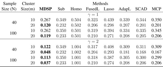
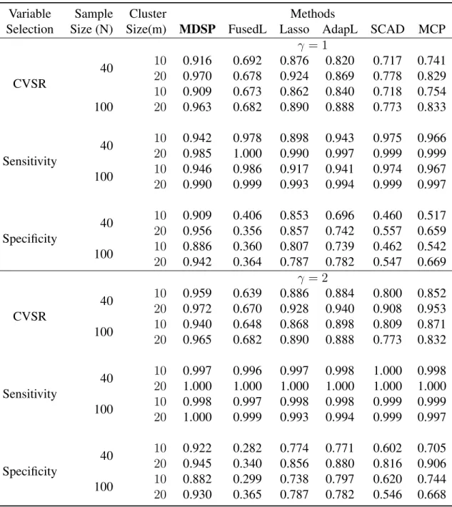
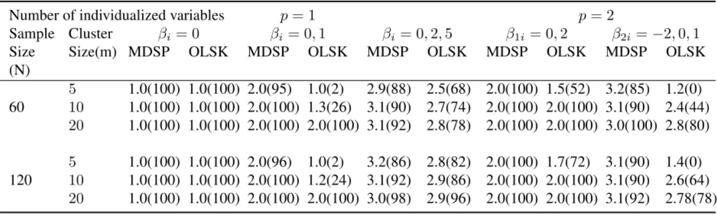
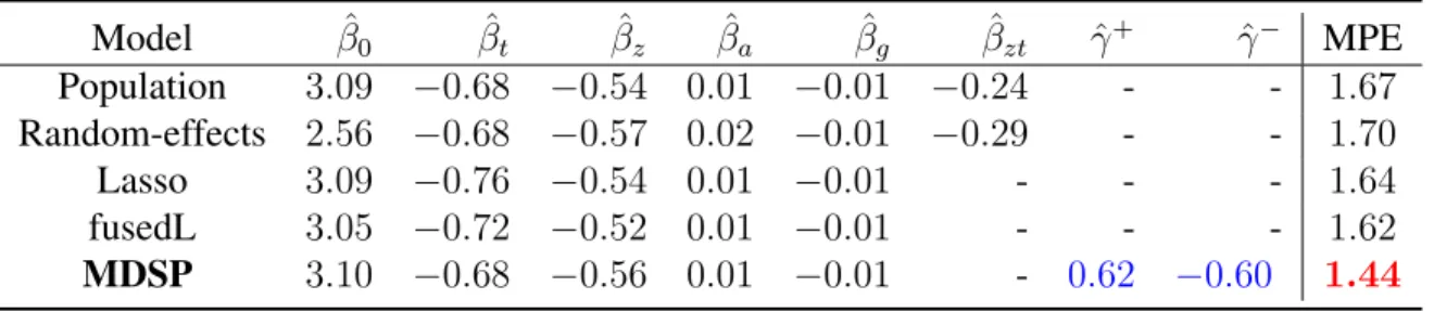
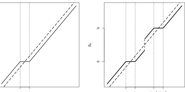
In Chapter 3, We propose a novel individualized variable selection method which performs coefficient estimation, subgroup identification and variable selection simultaneously. In contrast to traditional feature selection approaches, an individualized regression model allows different individuals to have different relevant variables. The key component of the new approach is to construct a multi-directional separation penalty which shrinks weak signals to zero and aggregates strong signals to a subgroup-shared homogeneous effect. This allows us to borrow information from subjects within the same subgroup, and therefore improve the estimation efficiency and vari-able selection accuracy for each individual. Another advantage of the proposed model is that it can incorporate within-subject correlation for longitudinal data.

We provide a general theoretical foundation under a double-divergence modeling framework where the number of subjects and the number of repeated measurements both go to infinity, and therefore involves high-dimensional individual parameters. In addition, we present the oracle prop-erty for the proposed estimator to ensure its optimal large sample propprop-erty. Simulation studies and an application to HIV longitudinal data are illustrated to compare the new approach to existing penalization methods.

1.3 Tensor Learning for Imaging Data Analysis

Imaging analysis has drawn great attention and encounters an explosive growth, due to wide ap-plications in medical images for diagnosing, especially in neuroimaging and cancer radiotherapy. It is in great demand to develop efficient statistical tools to utilize the image information to predict interested outcomes, for example, disease status and treatment responses. However, the imaging data has many challenges to be fitted into a traditional statistical model, including high-dimensional data structure, heterogeneous background noise and multiple data modalities.

Chapter 4 is motivated by multiphoton optical imaging data for breast cancer diagnosis pro-duced by Boppart Lab at University of Illinois at Urbana-Champaign, where there are four

(12)

imag-ing modalities at each subject capturimag-ing different microenvironments. In Chapter 4, we treat the image data along with additional information (e.g., time) as a higher-order multi-dimensional ar-ray, which is called a tensor as well. We propose a multi-layer tensor learning model to efficiently extract image’s information and then use the extracted information to fit a regression model as-sociated to the interested outcomes. Specifically, we construct a low-rank decomposition for the image tensor, which consists of the individualized layers, which capture the subject-specific infor-mation over each individual’s multiple modalities, and the population-shared layers, which model the modality-specific background and achieve an effective dimension reduction. Then the both layers’ information are incorporated to predict the outcome responses.

Due to individualized signals, traditional homogeneous dimension reduction methods could loss their power in capturing those images’ structures under a conventional low-rank model frame-work. By decomposing a tensor into different specific layers, the proposed method is capable of capturing the unique spatial information from the tensor structure and reduces the complex data’s dimensionality efficiently. Numerical studies illustrate the power of the proposed method, especially when signal regions vary a lot among different images, which often occurs in breast cancer diagnosis. The proposed approach is also applied to four-modality optical imaging data and achieves a significantly better prediction power on breast cancer diagnosis.

(13)

Chapter 2 Mixture Modeling for Longitudinal Data

2.1 Introduction

The mixture model has been extensively applied in many fields due to its flexibility to capture the heterogeneity arising from subgroups (components) in the whole population. The mixture model can also be viewed as a two-level hierarchical structure with incomplete data, where the first level consists of latent variables indicating subjects’ subgroup memberships, and the second level consists of outcome variables. However, the individual’s subgroup membership has to be inferred from the location of the outcome response due to unobservable latent variables.

Existing methods of mixture model with covariates for independent data include, but are not limited to, [30]’s mixture-of-experts for a mixture of component regressions, [32]’ extension on the generalized linear model for mixing proportion. For correlated or longitudinal outcome data, [70] introduce a linear random-effects model for components’ densities under the mixture frame-work. Alternatively, [67] propose a generalized estimating equation for component distributions to incorporate correlations. These approaches all assume that the latent variables are independent. However, modeling correlation from outcome variables only is not sufficient to address correla-tions from subgroup membership over time.

One notable approach to model the correlated latent structure is the hidden Markov chain model ([62]). However, this is not applicable for longitudinal data since the Markov chain assumption dose not hold or approximate some common correlation structure in longitudinal data such as exchangeable structure. Another well-known approach of mixture modeling for longitudinal data is related to growth-curve mixture modeling [53], where the subject’s group membership is fixed

(14)

over time, while different trajectory classes represent different mixture components. [29] propose a kernel smoothing method for a mixture of Gaussian processes incorporating both functional and heterogeneous types of dense longitudinal data. In addition, to incorporate the individual effects, [80] propose a multivariate Bernoulli mixture model by utilizing random effects in the generalized linear model for mixing proportion.

Although the mixed-effects model is widely used to handle dependent data, incorporating serial correlation for latent variables in mixture modeling for longitudinal data is still limited. In this chapter, we are interested in developing an efficient method in mixture modeling of longitudinal data where within-subject subgroup memberships could be correlated.

One challenge in formulating a mixture model for dependent data is that the joint likelihood function usually does not have an explicit form, because the latent variables are correlated categor-ical variables. In addition, the latent indicator variables are unobservable and require imputation. Although one can assume independent structure for the latent variables, the estimation efficiency will be compromised.

In this chapter, we allow group memberships to change over time in addition to taking serial correlation into account. We adopt the generalized estimating equation (GEE) approach ([44]) for both component distributions and mixing proportion in a two-component mixture model. This can be accomplished by treating the estimating equations for incomplete data as the conditional ex-pectations of those for complete data. Specifically, we apply the Expectation-Estimating-Equation (EEE) algorithm to solve the equations. To impute the latent variable in the E-step, we provide an approximation method to calculate the joint conditional expectation utilizing the conditional linear property for the correlated binary variables ([61]; [63]).

In contrast to the joint likelihood approach, the proposed method only requires the marginal distributions for both components’ densities and latent variables. In the estimating step, we fully utilize the serial correlation while treating it as a working structure. Allowing different working correlation structures enables one to incorporate various correlated latent structures, although the proposed method does not require to know the true correlation structure in order to produce

(15)

con-sistent estimators of mean parameters. However, if the correlation structure is correctly or closely specified, we gain efficiency of the parameter’s estimation and improve the classification accuracy from a model-based clustering.

The rest of this chapter is organized as follows: Section 2.2 introduces some notation and background knowledge; Section 2.3 presents our method and provides some theoretical results, as well as the EEE algorithm and imputation methods; Section 2.4 provides simulation studies; Section 2.5 considers an application to the Election data; and Section 2.6 offers a brief summary and some further discussion.

2.2 Background and Notation

For longitudinal data, let yit be the response of subject i at time t, and xit be a p-dimensional covariate vector, wherei= 1, ..., nandt = 1, ..., Ti. For ease of notation, we first assumeTi =T for allirepresenting a balanced data case, where an unbalanced data case will be discussed later. Denoteyi = (yi1, ..., yiT)as aT×1response vector,xi = (xi1, ...,xiT)as ap×T covariate matrix. In a two-component mixture model, letzitdenote the binary latent variable associated withyit. Let µr(·)be an inverse link function satisfyingE[yit|xit, zit = 2−r] = µr(βr0xit)(r = 1,2), where

βris a p-dimensional parameter, andµri =E[yi|xi,zi =2−r].

In this chapter, we consider a two-component mixture model. The outcome variableyitis from either one of the two subgroup populations and thus is assumed to follow a mixture distribution πitf1(yit|xit,β1, φ1) + (1−πit)f2(yit|xit,β2, φ2), whereπitis a mixing proportion defined as the probability of a responseyit from a specified subgroup,f1(yit|xit,β1, φ1)andf2(yit|xit,β2, φ2)

are the components’ distributions, and φ = (φ1, φ2) is the dispersion parameter. This

two-component mixture model can be regarded as a hierarchical structure. Specifically,

zit∼Bernoulli(πit),

(16)

where a latent variablezitrepresents a subgroup membership indicator.

The most common assumption for this hierarchical model is that the outcome variable yit’s are conditionally independent given the subgroup membership labelzit, then the joint likelihood density function of complete data(yi,zi)can be written as

Under the mixture framework, the latent variablezitis missing. The simplest way to get around the latent structure is to assume independence of subgroup memberships at different times within each subject and thus p(zi|πi) =

QT t=1π

zit

it (1 −πit)1−zit. In the independent mixture model, the correlations among longitudinal observations and their subgroup memberships are not fully utilized.

[32] propose a hierarchical mixture-of-experts model which takes covariates into consideration for both latent variable and component distributions, where the latent variable zit is assumed to follow a logistic model: πit = exp(η0xit)/(1 +exp(η0xit)), and components’ densities have a

mean regression form. Here we denoteθ = (η0,β₁0,β₂0)0 as a grand mean parameter vector, then the log of joint likelihood for complete data is:

Lc(y,z,θ,φ) = n X i=1 T X t=1

zit{logπit+logf1(yit|xit,β1, φ1)}+ (1−zit){log(1−πit)

+logf2(yit|xit,β2, φ2)}

,

(2.2)

under the independence assumption within subject.

For classical mixture models where the latent variablezitis missing, the maximum likelihood estimator (M LE) is typically computed through the Expectation-Maximization (EM) algorithm ([12]). The EM algorithm proceeds iteratively in two steps. In the E-step, we take the conditional expectation of complete-data log likelihood given observed outcome response y and current pa-rameters’ estimates(θ(k)_,_φ(k)₎_{. Since the complete-data log likelihood}_L

c(y,z,θ,φ)in (2.2) is a linear function of latent variablezit, the E-step only requires us to imputezitby its conditional

(17)

ex-pectationw_it(k) =E[zit|yit,xit,θ(k),φ(k)]denoted as the mixing weight. In the M-step, we obtain

thek+ 1th updates of parameters’ estimations by maximizing

L(θ,φ|θ(k),φ(k)) = n X i=1 T X t=1

w_it(k){logπit+logf1(yit|xit,β1, φ1)}+ (1−wit(k)){log(1−πit)

+logf2(yit|xit,β2, φ2)}

. (2.3)

It has been shown that the obtained series(θ(k),φ(k))in the EM algorithm converges to theM LE estimator of the mixture distributionf(y,θ,φ) =R_zfc(y,z,θ,φ)dz([12]).

2.3 Unbiased Estimating Equations for Mixture Modeling

2.3.1 Unbiased estimating equations

Due to the correlated nature of longitudinal data, it is important to incorporate correlation for mix-ture modeling as it provides more efficient estimation and benefits the longitudinal subgrouping. In this section, we first propose an efficient unbiased estimating equation for complete data, and then extend it to the incomplete-data mixture model.

To account for within-subject correlation among group memberships in (2.1), we have to deal with the joint likelihood function p(zi|πi) of the latent multivariate Bernoulli variable zi.

Un-like the multivariate Gaussian distribution, there is no explicit form of Un-likelihood function for the multivariate Bernoulli distribution. The unknown membership in the mixture models makes the incomplete-data likelihood function even more complicated since the latent zi needs to be

inte-grated out from the complete-data likelihood function. One possible approximation is to apply the Bahardur representation ([1]) for the multivariate Bernoulli distribution by ignoring high-order moments. However, there are several drawbacks such that the correlations are constrained through marginal means and covariates in a complicated way ([15]). In addition, the dimension of the correlation parameters could be very high when the repeated measurement sizeT is large, which leads to increasing computational demands.

(18)

To address this problem, we first introduce an unbiased estimating equation approach and es-tablish it for the complete-data model. The proposed unbiased estimating equation regrading the mean parameter θ is formulated through the log-likelihood functionLc in (2.2). MaximizingLc with respect toθ by solving the corresponding score equation is equivalent to solving the quasi-likelihood equation ([89]; [51]) as follows:

Sc(θ) = n X i=1 S_ic(θ) =       Pn i=1 ∂πi ∂η T V_i−1(zi−πi) Pn i=1 ∂µ1i ∂β1 T U1i−1Zi(yi −µ1i) Pn i=1 ∂µ2i ∂β2 T U2i−1(1−Zi)(yi−µ2i)       = 0, (2.4)

where µri = (µri1, ..., µriT)0, µrit = E[yit|zit = 2−r] = µr(βr0xit) (r = 1,2) are the

corre-sponding mean functions for components’ densities,Zi =diag(zi1, ..., ziT)is a diagonal matrix of corresponding latent labels, and U1i and U2i are the diagonal covariance matrices of component densities respectively: Uri = Var(yi|zi = 2−r). The covariance matrices U1i and U2i could be functions of both mean parameters µ1i, µ2i and dispersion parameter φ. As a result, given

θ, the dispersion parameterφcan be consistently estimated via the second moment conditions of component distributions. For the independent model,Vi =diag

Var(zi1), ...,Var(ziT)

. To account for serial correlation induced by latent variablezi, we assumeVi = A

1 2 i R(ρ)A 1 2 i

analogue to the generalized estimating equation (GEE) ([44]), whereAi =diag{πi1(1−πi1), ..., πiT(1− πiT)}is a diagonal matrix of marginal variance ofzi, andR(ρ)is a working correlation matrix. IfRis the true correlation matrix forzi, thenVi =Cov(zi).

In the following, we extend the proposed estimating equation to the incomplete-data model. To handle the missing latent indicatorzi, we take the conditional expectations for the equations in

(19)

for the incomplete data as: S(θ) = Ez[ n X i=1 S_ic(θ)|y,θ] = n X i=1 Si(θ|θ) =       Pn i=1 ∂πi ∂η T V_i−1(wi−πi) Pn i=1 ∂µ1i ∂β1 T U1i−1Wi(yi−µ1i) Pn i=1 ∂µ2i ∂β2 T U2i−1(1−Wi)(yi−µ2i)       = 0, (2.5) wherewi =Ez[zi|y,θ]is the mixing weight representing the inferred probability of the subgroup

memberships, andWi is a diagonal matrix of corresponding mixing weights associated withyi.

Similar to the GEE method, our approach can handle unbalanced data if the missing mechanism is missing completely at random (MCAR) ([69]). If the missing mechanism is not MCAR, then the estimating equation estimators could be biased and inefficient, and weighted generalized estimat-ing equations (WGEE) can be employed to deal with the missestimat-ing not completely at random cases ([66]; [68]).

To solve the estimating equation (2.5), we present a two-step Expectation-Estimating-Equation (EEE) algorithm. Analogue to the EM algorithm, the EEE algorithm follows an iterative estimating process. Specifically, at the(k+ 1)th step, based on the current estimation of parameterθ(k)_{, we}

imputew_i(k)=Ez[zi|y,θ(k)], and then updateθ(k+1)by solving the estimating equation:

S(θ|θ(k)) = n X i=1 Si(θ|θ(k)) =       Pn i=1( ∂πi ∂η) T_V−1 i (w (k) i −πi) Pn i=1( ∂µ1i ∂β1) T_U 1i−1W (k) i (yi−µ1i) Pn i=1( ∂µ2i ∂β2) T_U 2i−1(1−W (k) i )(yi −µ2i)       = 0. (2.6)

A more detailed EEE algorithm is provided in Section 2.3.3.

The main difference between the above method and [67]’s approach is that we incorporate an additional estimating equation associated with the mixing proportion. This enables us to utilize the longitudinal correlations among the unobservable subgroup memberships from the same subject. Furthermore, in our estimating equation (2.5), we can also utilize the correlation information from the outcome variableyisimultaneously through the working correlation structures ofU1i andU2i.

(20)

assume that yit’s givenzit’s are conditionally independent within the same subject, and thusU1i andU2i are set to be diagonal.

Indeed, the proposed model assuming working correlation structure has the same identifiability problem as the independent model, which is equivalent to the mixtures-of-experts model. We can refer to [31]’s discussion for the identifiability problem of the mixtures-of-experts model.

2.3.2 Asymptotic Properties

In this chapter, we utilize the latent variable’s serial correlation information to improve the param-eter estimation and the subject’s group membership prediction. We first examine the optimization properties for the complete-data equations.

Once we establish the optimal estimating equationSc(z,y,θ)for complete data, then the con-ditional expectationS(y,θ) =E[Sc_|_y_]_{is the best estimating equation for the incomplete data such} that theL2normkSc(z,y,θ)−S(y,θ)kis minimized. In other words, if the proposedSc(z,y,θ)

is efficient enough, then S(y,θ) will inherit some efficiency from the complete-data model. In the following proposition, we establish the optimality of the unbiased estimating equation (2.4) for complete data.

Proposition 1. If the working correlation structure is correctly specified, that is,Vi =Var(zi), the estimating equations in (2.4) are the optimal linear estimating equations with respect to (zi,yi),

in the sense that the asymptotic variance of the estimator solved by (2.4) reaches the minimum.

The proof is provided in the Section 2.7. Indeed, incorporating the serial correlation informa-tion is more important for the mixture model sincezi can not be observed. For the complete-data

estimating equations in (2.4), the first set of equations with respect to the group membership and the other two equations associated with component densities are uncorrelated with each other. Therefore the induced serial correlations only affect the estimation of mixing proportion param-eters in π(η), but have no influence on estimating the component parameters in µ1(β1) and

(21)

imputed termwiis a function ofyi. For the longitudinal data of the subjects, taking advantage of

the information at the other time points through accounting for the serial correlation improves the estimation efficiency of both the component parameters and the mixing proportion parameters.

It is known that the consistency of the above estimator only depends on correct specification of the mean functions, but does not rely on correct specification of the working correlation struc-ture nor on the estimation of the correlation parameters ρ. This is one desirable property for the proposed approach since the serial correlation induced from unobservable latent variables could be difficult to model and estimate precisely. In contrast to the full joint likelihood approach, we only require the second moment approximation. Furthermore, the following theorem establishes the asymptotic properties of the proposed estimators.

Theorem 1. Letγ = (θ0,φ0)0denote a grand parameter vector, in the proposed unbiased estimat-ing equation (2.5), assumestimat-ing that the followestimat-ing regularity conditions are satisfied:

(i)φˆis consistently estimated givenθ via some unbiased estimating equationPn

i=1Hi(φ|θ) = 0; (ii)ρˆisn1/2-consistent givenγ, denoted asρˆ(γ);

(iii)k∂ρ/∂ˆ γk ≤Op(1);

LetGi(γ) = (Si(θ)0, Hi(φ|θ)0)0be the augmented unbiased estimating equation, then the asymp-totic distribution ofγˆ obtained fromPn_i₌₁Gi = 0is: n1/2(ˆγ−γ)→N(0, Vg), where the asymp-totic covariance matrixVg is given by:

Vg =limn→∞n n X i=1 ∇Gi(γ) −1 n X i=1 cov(Gi(γ)) n X i=1 ∇Gi(γ) −T ,

∇Giis the gradient ofGi with respect toγ.

Theorem 1 is established based on the following unbiased estimating equations:

E[(wi−πi)] =E[(E[zi|yi]−πi)] =E[zi]−πi = 0;

E[Wi(yi−µ1i)] =E[E[Zi|yi](yi−µ1i)] =E[Zi(yi−µ1i)] = 0; E[(1−Wi)(yi−µ2i)] =E[(1−E[Zi|yi])(yi−µ2i)] =E[(1−Zi)(yi−µ2i)] = 0.

(22)

A sketch of the proof of Theorem 1 is given in the Section 2.7. Noting that even ifwi is imputed through the marginal expectationwit = E[zit|yit], the estimating equations in (2.5) are still unbi-ased. The estimating equationHi for the dispersion parameter is established based on the second moment condition provided in the Section 2.7.

In practice, a consistent variance estimator ofγˆ can be obtained by replacing Cov(Gi(γ))by

ˆ

G_i0Gî, and∇Gi by∇Gî at the estimates ofθˆ,ρ,ˆ φˆ. One practical difficulty arises from getting an explicit form of the gradient∇Gîin the calculation of mixing weightswi. The imputation termwi is the posterior probability ofzicontaining both the response valueyi and all the parametersθ,φ andρ. The complicated form ofwi makes it difficult to calculate the exact derivatives, especially when the conditional expectationwi = E[zi|yi]requires specifying the joint likelihood function forzi. We present some numerical approximation methods to calculatewi and∇Gi. More details are provided in Section 2.3.3.

2.3.3 Algorithm and Implementation

In this section, we provide the two-step iterative EEE algorithm and its theoretical properties. In addition, the details of marginal imputation and the joint imputation methods are provided.

Algorithm 1

Step 1: Set the initial values of the mean regression parameterθand the dispersion parameterφ:

γ(0) = (θ(0),φ(0));

Step 2 (E-Step): Impute the mixing weightsw(_itk) =E[zit|yi]given current estimatesγ(k);

Step 3 (M-Step): Given the current imputed mixing weightsw(_itk), (i) updateθ(k+1) by solving the estimating equation in (2.6), and (ii) updateφ(k+1) _given_θ(k+1)_;

Step 4: Return to Step 2 ifkγ(k+1)₋_γ(k)_k_>_{, where}_{is the chosen tolerance level.}

In Step 3 of Algorithm 1, with the current mixing weights, we apply the Newton-Raphson method to solve the estimating equations in (2.6) to obtain the updates θ(k+1) for the mean pa-rameter. The updated dispersion parameter φ(k+1) _{can be estimated using the second moment}

conditions givenθ(k+1)_{. See Section 2.7 for more details. In the Newton-Raphson algorithm, the}

(23)

diag Pn i=1 ∂πi ∂η T V_i−1 ∂πi ∂η ,Pn i=1 ∂µ1i ∂β1 T U1i−1W (k) i ∂µ1i ∂β1 ,Pn i=1 ∂µ2i ∂β2 T U2i−1(1−W (k) i ) ∂µ2i ∂β2 .

For the EEE Algorithm 1, the estimating function in (2.5) can be regarded as a bivariate func-tion S(θ|λ) restricted on the subspace θ = λ, which is denoted as S(θ|θ). In fact, the first argument θ of S(θ|θ) comes from the mean regression part, while the second argument comes from the conditional expectations. The EEE Algorithm 1 is simply updating the estimation ofθ

by solvingS(θ|θ(k)_{) = 0}_{in (2.6). If the iterative sequence of the estimator obtained from the EEE}

algorithm converges, it will converge to the solution of the original equationS(θ|θ) = 0which is guaranteed by the continuity. The following lemma provides a local convergence of the estimator based on the Algorithm 1 in a more general form.

Lemma 1. Suppose thatS(θ|λ)is a bivariate function on the spaceΘ×Θsatisfying the following regularity conditions:

(a)S(θ|λ)is continuous and both ∂S_∂_θ and _∂∂S_λ exist;

(b) In a neighborhood of(θ0,θ0), whereS(θ0|θ0) = 0, we havek(∂S_∂_θ)−1· ∂S_∂_λ k2<1hold;

then the iterative sequence of estimator{θ(k)_}_{solved by}_S₍_θ(k+1)_|_θ(k)_{) = 0}_{converges to}_θ

0.

The proof of Lemma 1 is provided in the Section 2.7. Lemma 1 provides a sufficient but not necessary condition for the algorithm’s convergence. Indeed, the algorithm convergence problem is also associated with general convergence theory regarding the iterative solutions to nonlinear equations. More detailed discussion of this type of algorithm can be found in [55].

In practice, it is possible to have multiple roots for the proposed estimating equations. One suggested method is to choose the root closest to the independent estimator which is consistent ([78]). [73] proposed to exclude all singular solutions and therefore reduce the risk of selecting spurious roots of the likelihood equation. Their method is powerful in selecting reasonable roots for the independent finite normal mixture model. In addition, we may also need to provide a “good” initial value for the iterations to converge. One way is to select different initial values randomly until the algorithm converges; another choice is to set the initial value as the estimator obtained from the existing independent mixture model.

(24)

In Algorithm 1, the E-step (Step 2) requires one to impute the missing latent variablezithrough

its conditional expectation wi = E[zi|y,θ,φ]. However, this joint conditional expectation

in-volves the joint density of the multivariate binary variablezi, which is very difficult to calculate.

One possible way is to use the marginal imputationwit = E[zit|yit,θ,φ]since we only assume a marginal distribution for the individual observation(yit, zit)in our approach. The marginal impu-tation

wit =

πitf1(yit,θ1, φ1)

πitf1(yit,θ1, φ1) + (1−πit)f2(yit,θ2, φ2)

guarantees the estimating equations in (2.5) to be unbiased, wheref1 andf2 are component

den-sities. In fact, the imputation wit provides the inferred subgroup membership of the outcome observationyit. The drawback of the marginal imputation is that it only utilizes local information to infer the group membership. If two subgroups are well-separated, i.e., mostwitare either close to 1 or 0, then the marginal imputation is sufficient since the local informationyit dominates the subgroup membership’s prediction. However, if two subgroups are not well-separated, then the marginal imputation does not fully utilize the within-subject correlation to improve the subgroup classification.

Therefore, we provide an alternative approximation of the joint imputation w∗_it = E[zit|yi]

which relies only on the second moment condition of zi. To predict the subgroup member-ship of yit, we consider the conditional expectation E[zit|yit,zi(−t)] based on local observation

yit and all latent group labels zi(−t) at other time points for the ith subject, where zi(−t) =

(zi1, ...zi(t−1), zi(t+1), ..., ziT). Since

P(zit|yit,zi(−t))∝f(yit|zit)P(zit|zi(−t)),

thenw∗_it=π_it∗f1(yit,β1, φ1)/[πit∗f1(yit,β1, φ1)+(1−π∗it)f2(yit,β2, φ2)], whereπit∗ =E[zit|zi(−t)].

By taking account ofzi(−t), this imputationwit∗ allows us to utilize the group membership infor-mation from other time points within the same subject as well.

(25)

Motivated by [61]’s conditional linear family for the multivariate binary distribution in generating correlated binary data, we consider a linear approximate:

π_it∗ =E[zit|zi(−t)] =πit+bTit(zi(−t)−πi(−t)),

whereπit =E[zit],πi(−t)=E[zi(−t)], andbit is a(T −1)-dimensional coefficient vector. Based

on the fact that for any two random variableX andY, Cov(X, Y) = Cov(X,E[Y|X]), we have:

Cov(zi(−t), zit) = Cov(zi(−t), πit∗) =Cov(zi(−t))bit.

Denote Cov(zi(−t), zit)assit and Cov(zi(−t))asVi(−t), thenbit =V_i−₍₋1_t₎sit. Here bothsit and

Vi(−t)could be obtained from the second moment condition Cov(zi).

To implement the Algorithm 1, at the (k + 1)th step, we use the current estimatorsθ(k) _and

V_i(₍k₋)_t₎to obtainπ_it∗(k+1) and thus imputew_it∗(k+1). Here the true latent labelzi(−t)is replaced by

the last predictionzˆ_i(₍k₋)_t₎. A similar technique is also used by [62] to approximateP(zit|ˆz

(k)

i(−t))in

a hidden Markov field modeling.

In Section 2.3.2, we mention that in order to obtain the robust variance estimator of γˆ, it requires us to calculate the gradient of Gi(γ). Here we take the numerical approximation of the gradient∇Gi(γ)by Gi(γ

(k+1)₎₋_Gi₍_γ(k)₎

γ(k+1)₋_γ(k) , whereγ

(k)_and_γ(k+1)_{are obtained from the previous two}

adjacent iterations, and the ijth component of ∇Gi(γ) corresponds to the ratio between the ith andjth components ofSi(γ(k+1))−Si(γ(k))andγ(k+1)−γ(k)respectively.

2.4 Numerical Study

In this section, we conduct two simulation studies to illustrate the performance of the proposed method on mixture modeling for longitudinal data. We are particularly interested in comparing the performance of our method to other approaches when the serial correlation is induced by latent variables. Our simulation results show that we can gain efficiency on parameter estimation by

(26)

utilizing correlation information.

In the first simulation study, we consider a two-component mixture of univariate normal dis-tribution, and mainly focus on the estimating performance of the mixing proportion parameters with different dependence structures. In the second simulation study, we consider a mixture of two regression models, where the separation levels of two subgroups will change over time. The proposed method has extra power in both estimation and prediction, especially at poorly-separated time points.

2.4.1 Study 1: Two-component mixture of univariate normal densities

In this simulation study, we first generate component indicator variablesZi from Bernoulli distri-butions for subjectsi = 1, ..., n. For eachZi, we assume there areT repeated measurements over time, where Zi = (Zi1, ..., ZiT), and Zit is a binary variable following a logistic regression with time covariate. That is,E[Zit] = πitandlog(₁₋πit_πit) =η0+η1_Tt. Conditional onZit, we generate

outcome response Yit from two univariate normal distributions: Yit|(Zit = 1) ∼ N(µ1, σ21) and

Yit|(Zit = 0)∼ N(µ2, σ22). For latent variableZi, we assume independence among different sub-jects, but a common correlation structure (either AR-1 or exchangeable) within a subject over time. For outcome response Yi, we assume independence among different subjects and conditional in-dependence within a subject given component indicatorZi. In our simulation studies, we generate binary responses through the R package “mvtBinaryEP”.

We let the sample sizen= 100and time pointsT = 10, and the mixing proportion parameters in the logistic model are set to be(η0, η1) = (−0.3,0.5), which allows certain correlations among

multivariate binary variables. In addition, we set variance parameters as(σ2

1, σ22) = (1,1).

The separation between two normal homoscedastic components could be accessed by ∆ =

|µ1−µ2|/σ, defined as the Mahalanobis distance between two normal mixture distributions ([52]).

We investigate two settings with component means(µ1, µ2) = (−1.5,1.5)and(µ1, µ2) = (−1.2,1.2)

to represent well-separated and poorly-separated bimodal densities, respectively. In addition, we also simulate a heterogeneous case with(µ1, µ2) = (−1.5,1.5)and(σ1, σ2) = (1,1.5). The

(27)

sim-ulation results are similar to those for the homogeneous case, and are thus omitted due to space limitations.

In the following simulation studies, we choose the initial value randomly in the neighborhood of the independent estimator until the EEE algorithm converges. The estimation results are sum-marized based on 1000 replicates. In our simulations, the empirical standard errors are quite close to the standard errors calculated from the robust sandwich variance, and therefore we only pro-vide the empirical standard errors in our tables. In practice, label-switching issues might arise, especially for Bayesian mixture models. [92] and [93] discussed many feasible labeling meth-ods. In our simulation study, we solve the labeling problem by imposing an ordered constraint on components’ mean parameters.

We compare the estimators based on the proposed unbiased estimating equation with either joint imputation (U EEJ oint) or marginal imputation (U EEM ar), with working correlation structure of either exchangeable, AR-1 or unstructured, the mixtures-of-experts model (Jacobs et al., 1991) which is the same as the independent estimating equation (U EEInd), and the oracle estimators (Oracle) assuming the true values of latent variableZiare known. The oracle estimator serves as a benchmark estimator, where the generalized estimating equation (GEE) utilizes the correlation structure for the binary dataZi, and the M LE estimators of component parameters are obtained given Zi. In the following tables, we denote the correlation structure in the superscript such as U EEAR1

J oint. In the text, to avoid redundant notation, we omit the superscript if the correlation structure is correctly specified.

In addition, we also compare the proposed method with the random-effects model ([80]. In the random-effects model, we assumeE[Zit] = πit andlog(₁₋πit_πit) = η0+η1_Tt +γi, whereγi ∼ N(0, σ2

γ) is the random intercept accounting for the subject effect. Givenγi, the latent variables within theith subject are independent. The random-effects estimator (RE) are obtained by the EM algorithm.

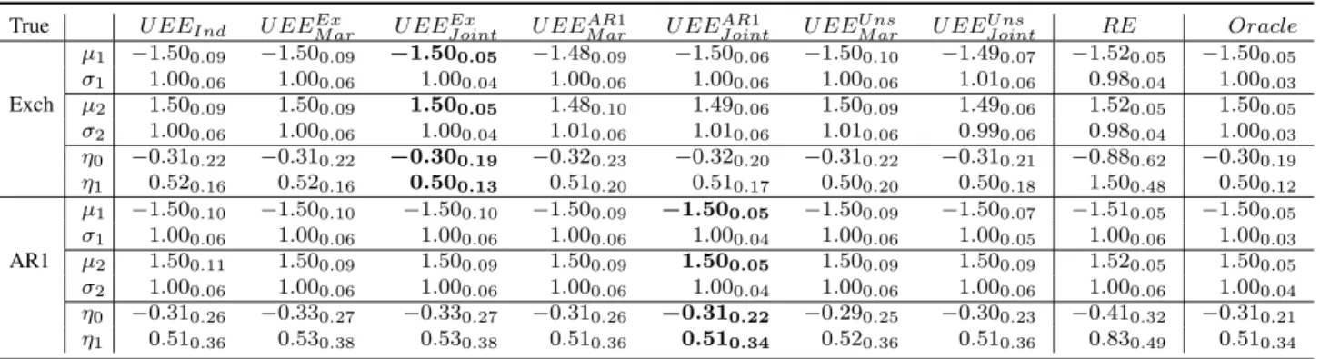
In Tables 2.1 and 2.2, we observe that all the estimating equation estimators are consistent as discussed in Section 2.3.2, including the estimators using misspecified correlation structures.

(28)

However, we can improve the estimating efficiency if the correct correlation information is in-corporated especially for joint-imputed model. This is reflected in that theU EEJ oint estimators have much smaller standard errors compared with the other estimators in both well-separated and poorly-separated cases. Indeed, theU EEJ oint performs almost the same as theOracleestimator. For a well-separated case or if an exchangeable correlation structure is assumed, the performance of theU EEM aris quite similar to that of theU EEIndsince the longitudinal data generated here is balanced ([44]). But when two subgroups are poorly-separated and the latent variable has an AR-1 correlation structure, then theU EEM ar has smaller standard errors thanU EEInd.

In addition, if we compare Table 2.1 and Table 2.2, we notice that the standard errors of the in-dependent estimators increase significantly from a well-separated case to a poorly-separated case, while the proposed U EEJ oint is much more stable and performs similarly to theOracle estima-tor. Table 2.3 provides the classification error rates from the model-based clustering. The proposed U EEJ ointmodel has sufficient power in predicting the subgroup membership since we incorporate the information from other time points for the same subject.

In general, it is difficult to know the true correlation structure for latent variables. The un-structured working correlation is always a possible choice because of its flexibility, as it does not assume any pattern for the correlation structure. However, the unstructured correlation leads to additional computational cost, as it has more correlation parameters T∗(T₂−1) to estimate compared with the AR-1 and exchangeable working correlations. In addition, the variation introduced by unstructured correlation leads to less efficient estimations for regression parameters and increases the chance of the convergence problem in the EEE algorithm. The unstructured model is recom-mended when the sample sizenis large and the repeated measurement sizeT is relatively small in the well-separated case. In Tables 2.1 and 2.2,U EEU ns

M arandU EEJ ointU ns do not show significant im-provement in estimations, but they have more power in prediction compared with the independent and misspecified models in Table 2.3.

In Tables 2.1-2.2, the random-effects estimators perform poorly with large bias and standard errors. This is because [80] approach can only incorporate the random intercept which might not

(29)

be sufficient to handle the within-subject dependence if group membership changes over time. In addition, we also conduct a simulation study where the latent variable Zi is generated from the random-effects model only (2.4). The random-effects model generates correlations which do not have an obvious patten. Therefore the proposed estimating equation assuming a certain pattern of working structure for serial correlations might not be the most efficient in estimation. Nevertheless, Table 2.4 indicates that although the standard errors of the estimating equation estimators are slightly overestimated, they are still acceptable. In all, regardless of which source the dependence within subjects is induced from, the proposedU EEestimators are robust and efficient in general.

2.4.2 Study 2: Two-component mixture of linear regression models

In simulation study 2, we consider a mixture of two linear regression models. In this case, not only the mixing proportion, but also the component densities follow a mean regression model with time covariates.

Similar to the first simulation study, we generate component indicator variables Zi’s from a logistic model, and for each Zi, we assume there are T repeated measurements over time with Zi = (Zi1, ..., ZiT). The mixing proportionE[Zit] =πitis generated from the logistic model:

log( πit 1−πit

) = η0 +η1

t T,

with either an AR-1 or exchangeable correlation structure. Conditional on Zit, we generate the outcome responseYitfrom two normal distributions:

Yit|(Zit= 1)∼N β₀(1)+β₁(1)t T, σ 2 1 , Yit|(Zit= 0)∼N β₀(2)+β₁(2)t T, σ 2 2 .

In this study, we let the sample size n = 100and time points T = 5, the mixing proportion parameters in logistic model are set to be(η0, η1) = (−0.3,0.5), and the component’s regression

parameters are set as (β₀(1), β₁(1)) = (−3,2) and (β₀(2), β₁(2)) = (3,−2), the variance parameters are set as (σ2_{, σ}2_{) = (1}_,₁₎_{. In contrast to the first simulation setting, the mixture components}

(30)

are regression functions of time covariates, where the component means are changing over time, leading to different separation levels at different times.

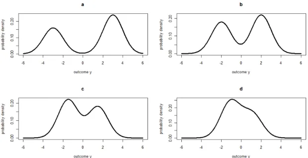
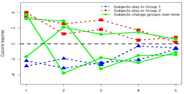
Figure 2.1 illustrates four different separations of two components at different time points in this simulation study. This motivates us to take advantage of serial correlations within subjects to improve accuracy in predicting class memberships and thus to improve the estimations of the regression parameters. In addition, we allow subjects to change group memberships over time (see Figure 2.2 as an illustration), which makes our approach more flexible compared to growth-curve mixture modeling.

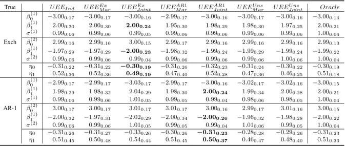
The results in Table 2.5 show that we gain extra efficiency with smaller standard errors in estimating both the mixing proportion parameters and the component regression parameters for the proposed U EEJ oint estimators especially on slope estimators. Table 2.6 indicates that our approach utilizing the within-subject correlation information provides more predictive power, es-pecially at poorly-separated times. In general, when within-subject correlation is large, our ap-proach is able to “borrow" information from well-separated observations to enhance membership prediction for poorly-separated observations by incorporating the correlations within each individ-ual subject. Consequently, improvement of the prediction of the subgroup’s membership leads to better estimation of the slope parameter associated with time effect.

2.5 Real Data Application: 2008 Election Data

In this section, we apply the proposed method to the 2007-2008 AP-YAHOO NEWS election panel study (http://www.knowledgenetworks.com/GANP/election2008/index.html). The study was con-ducted by Knowledge Networks on behalf of the Associated Press and Yahoo! News (APYN) which intends to measure opinion changes starting with the primary elections through the presi-dential election in November 2008. The data consists of 4965 participants over eleven waves from November 2007 to December 2008, with nine waves before the election, one wave on election day, and the last wave after the election. The primary goal of the study is to investigate the change of

(31)

participants’ interest in the election over time and important factors associated with their interest. One important factor associated with the interest in the election is interest in election news.

Therefore we choose one of the survey questions: “Question LV3: How much interest do you have in the following news about the campaign for president, a great deal, quite a bit, only some, very little, or no interest at all.” The five categories of opinions are recorded as an ordinal response variable: 1, 2, 3, 4 and 5, where a smaller value corresponds to a high level of interest in the election news. In order to measure the opinion change towards the election, we focus on the first nine waves occurring before the election date. There are 1200 participants who have completed the “Question LV3” over the first nine waves. In the following, we haven = 1200and the repeated measurement sizeT = 9.

In this study, we intend to classify all the participants into two groups, whether they actively follow the election or not, based on their responses to the question “LV3” in the AP-Yahoo sur-vey. Since the survey collects participants’ responses longitudinally, it is not surprising that their interest towards the election could be different at different time points. Consequently, this results in changes of group membership over time. The covariates include time, gender and race, where gender is 1 for female and 0 for male, and “race” consists of “white,” “black” and “the other” coded as dummy variables with “white" as the reference. In addition, we also include an interaction term between “time” and the “gender.”

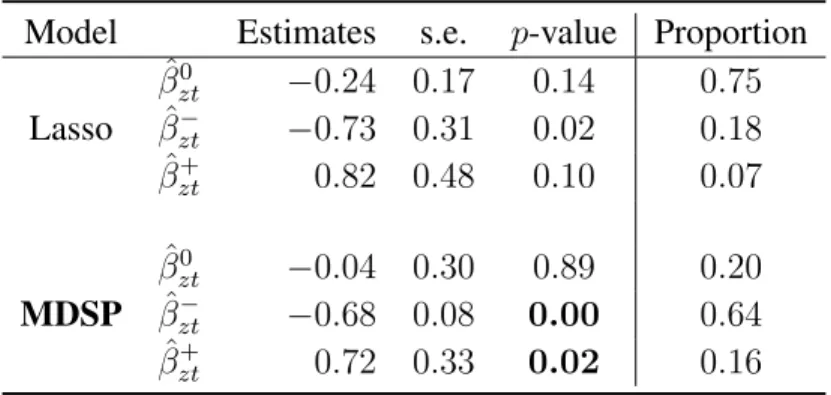
We formulate a two-component mixture model as follows. Let the latent variable Zitindicate whether the participantiat the time pointtis interested in election news (Zit = 1) or not (Zit = 0). We model the mixing proportion using a logistic regression to capture the change in group mem-bership, and the univariate Gaussian for the component distribution. We compare estimators via the proposed unbiased estimating equations using different working correlation structures: inde-pendent (U EEInd_{), exchangeable (}_{U EE}Exch_{), AR-1 (}_{U EE}AR1_{) and unstructured (}_{U EE}U ns_{), in} addition to the random-effects model (RE). The joint imputation is applied in all cases. We fo-cus on modeling the mixing proportion since we are interested in opinion changes over time. The estimates of mixing proportion parameters with correspondingp-values are summarized in Table

(32)

7. Thep-values are calculated based on the asymptotic normal distribution since the sample, size n= 1200is quite large.

Table 2.7 indicates that the participants become more and more interested in the election cam-paign as the time gets closer to election day. Male participants are more interested in election news than females on average; however, females become increasingly more interested in election news than their male counterparts as the election gets closer. In addition, the “black” group is more interested in election news compared to the “white” group, while the “other” group is slightly less interested in election news than the “white” group. In total, about 43.5% of the participants changed their group memberships of showing interest in election news over time.

Furthermore, Table 2.7 shows that the proposed estimating equation estimators using differ-ent working correlations are similar in iddiffer-entifying the effects for “gender” and the interaction of “gender” and “time,” which are highly significant. However, the estimators for the gender and the interaction term are not significant using the random-effects model with much largerp-values. In addition, the [59] reports that the “race” factor played a significant role in the 2008 presidential election, where “black" voters showed more interest in the election than other races in general. For this survey study, the “black” group is only about 7.5% of the participant population (90 out of 1200) which makes it more difficult to detect the “race” factor. Neither the random-effects model nor the independent estimating equations are able to detect a significant difference between the “black” group and the “white” group. However, the proposed method using the unstructured cor-relation is capable of identifying that the “black” group is significantly different from the “white” group with ap-value of 0.04. This implies that the proposed method accounting for the serial cor-relation can improve the estimation efficiency and increase testing power to detect a factor which might not be picked by other approaches.

(33)

2.6 Discussion

In this chapter, we propose an unbiased estimating equation approach for mixture modeling in longitudinal data, and illustrate how to induce correlation at the level of latent subgroup indicator variables. The proposed method does not require that each subject belong to the same group at dif-ferent time. To circumvent the complicated form of joint likelihood of the multivariate Bernoulli variables, we propose an unbiased estimating equation approach utilizing the first two moment ap-proximations of the full likelihood, where the serial correlation is incorporated through a working correlation structure. The proposed estimating equations can be regarded as a projection of optimal estimating equations obtained from the complete data via taking the conditional expectation for the missing latent variables.

Our numerical studies show that incorporating correlation information allows one to gain esti-mation efficiency for the mean regression parameters and the mixing proportion parameters com-pared to the independent models. The efficiency improvement is significant if the correlation from the longitudinal data is strong and the working structure is correctly specified. In addition, we can improve the classification accuracy for the boundary observations through joint imputation for the missing latent variable.

We can further generalize the current method for more than two subgroups in the population through the extended generalized estimating equation, applying the cumulative logit model for a multinomial latent variable. In addition, we can extend the univariate outcome variable to the mul-tivariate component distribution. If the dimension of the mulmul-tivariate distribution is high, we can employ the variable selection method by incorporating some penalty terms ([90]. In this chapter, we mainly focus on modeling serial correlation arising from the latent variable, it would be worth-while to consider a more complicated setting where within-subject dependence is induced by both latent variable and outcome variable.

(34)

2.7 Proofs of Theoretical Results

A.1 Estimate dispersion parameter

The dispersion parameter φ = (φ1, φ2)is associated with the second moments of the

compo-nents’ distributions. For compocompo-nents’ densities in the exponential family, we have

Var(yit|zit = 2−r) =ν(µrit)φr,r= 1,2. In the complete-data case, given the true subgroup label zit, for instance, the second moment of the first component distribution could be estimated by

c Var(yit|zit = 1) = Pn i=1 PTi t=1zit(yit−µ1it)2/ Pn i=1 PTi

t=1zit.Then we could establish an unbi-ased estimating equation forφ1given mean parameterµ1it(β1):

n X i=1 H_ic(φ1|β1) = n X i=1 Ti X t=1 zit[(yit−µ1it)2−ν(µ1it)φ1] = 0.

Similarly, we could establish the unbiased estimating equation for incomplete data by taking the conditional expectation: n X i=1 Hi(φ1|β1) = n X i=1 Ti X t=1 wit[(yit−µ1it)2−ν(µ1it)φ1] = 0,

wherewitis the imputed mixing weight, andφ2 is estimated in the same way.

For example, in the two-component Gaussian mixture model, the variance parameter(σ2₁, σ₂2)

for normal components could be estimated byσˆ12 =Pn_i₌₁PTi_t₌₁wit(yit−µ1it)2/Pn_i₌₁PTi_t₌₁wit. A.2 Proof of Theorem 1

Note that the estimating equation Gi in (2.5) contains both interest parameter γ = (θ0,φ0)0 and nuisance correlation parameterρ. By assumptions, the correlation parameterρcould be esti-mated consistently givenγ, written asρˆ(γ). Then the augmented unbiased estimating equation in Theorem 1 has the form

n

X

i=1

ˆ

(35)

From the theory of unbiased estimating equations ([25]), under some regularity conditions,n1/2_(ˆ_γ₋ γ)could be approximated by the one-step Taylor expansion:

[−n−1 n X i=1 dGi dγ ] −1_·_[_n1/2 n X i=1 ˆ Gi], where dGî(γ,ρˆ(γ)) dγ = ∂Gî(γ,ρˆ(γ)) ∂γ + ∂Gî(γ,ρˆ(γ)) ∂ρˆ · ∂ρˆ ∂γ.

With marginal imputation wit = E[zit|yit], the nuisance parameter ρ is only contained in the working correlation matrix R, therefore ∂Giˆ (_∂γ_ρ,_ˆρˆ(γ)) is linear of unbiased estimating equa-tions (wi −πi), thus Pn_i₌₁ ∂

ˆ

Gi(θ,ρˆ(γ))

∂ρˆ = op(n), and by condition (iii) k

∂ρˆ ∂γk = Op(1), therefore n−1Pn i=1 dGiˆ (γ,ρˆ(γ)) dγ =n −1Pn i=1 ∂Giˆ (γ,ρˆ(γ)) ∂γ +op(1).

Further, fixγand from Taylor expansion again:

n−1/2 n X i=1 ˆ Gi(γ,ρˆ) = n−1/2 n X i=1 Gi(γ, ρ) + [n−1 n X i=1 ∂Gi(γ, ρ) ∂ρ ]·[n 1/2_{( ˆ}_ρ₋_ρ_{)] +}_o p(1).

By condition (ii)n1/2( ˆρ−ρ) =Op(1)and alson−1

Pn i=1 ∂Gi(γ,ρ) ∂ρ =op(1), suggests thatn −1/2Pn i=1Gˆi(γ,ρˆ) is asymptomatically equivalent ton−1/2Pn i=1Gi(γ, ρ). Hencen 1/2_{( ˆ}_θ₋_θ₎_{could be approximated} by [−n−1 n X i=1 ∂Gi ∂γ ] −1_·_[_n1/2 n X i=1 Gi],

which would be asymptotically Gaussian with mean vector of0and asymptotic variance ofVg. A.3 Proof of Proposition 1

It is well-known from the theory of optimal estimating equations ([25]), that for unbiased estimating equation gi(θ), the optimal weights would be Var(gi)−1g˙i, where g˙i = ∂gi_∂_θ, θ0 =

(36)

(η0,β1,β20)

0

. As for the complete data(yi,zi), the unbiased linear equation is

gi =        zi−πi(η) Zi yi−µ1i(β1) (1−Zi) yi−µ2i(β2)        .

Firstly, it is easy to show thatg˙i has the form

˙ gi =       ∂πi ∂η 0 0 0 Zi∂_∂µ_β1i 1 0 0 0 (1−Zi)∂_∂µ_β2₂i       .

Also we could show that Var(gi)is a diagonal matrix

Var(gi) =       Var(zi) =Vi 0 0 0 Var(Zi(yi−µ1i)) 0 0 0 Var((1−Zi)(yi−µ2i))       . This is because E[(zit−wit)zij(yij −µ1ij)] =E (zit−wit)zijE[(yij −µ1ij)|(zit, zij)] = 0

always holds for anyt andj sinceE[(yij −µ1ij)|(zit, zij)] = (1−zij)(µ2ij −µ1ij). In addition, from the joint log-likelihood function (2.2) we could see that the component densities are estimated given the true values of latent variable in the complete-data case, and thus Var(Zi(yi −µ1i)) =

ZiU1iZiT. Noting that Zi is a diagonal matrix and U1i,U2i are diagonal covariance matrices,

thereforeZ_iTVar(Zi(yi−µ1i))−1Zi =U1−i1Ziand(1−Zi)TVar((1−Zi)(yi−µ2i))−1(1−Zi) =

U₂−_i1(1−Zi). Then the optimal equation has the form (2.4). A.4 Proof of Lemma 1

(37)

Consider the bivariate functionS(θ|λ)onΘ⊗Θ, we have the first order partial Taylor’s expansion with respect toθin a neighborhood of(θ0,θ0):

S(θ|λ)≈S(θ0|λ) +

∂S(·|λ)

∂θ ·(θ−θ0).

If we obtainθˆby solving the equationS(θ|λ) = 0, then( ˆθ−θ0)≈(∂S(

·|λ)

∂θ )

−1_·_S₍_θ

0|λ).

Apply partial Taylor’s expansion again with respect toλ:

S(θ0|λ)≈S(θ0|θ0) +

∂S(θ0|·)

∂λ ·(λ−θ0),

which indicates that( ˆθ−θ0)≈A(λ−θ0), whereA = (∂S(

·|λ)

∂θ )

−1_·∂S(θ0|·)

∂λ . Therefore we have

kθˆ−θ0 k≤kAk · kλ−θ0 k.

Hence, the iteratively constructed sequence{θ(k)_}_satisfies_k_θ(k+1)₋_θ

0 k≤kAk · kθ(k)−θ0 k

(38)

2.8 Tables and Figures

Table 2.1: The parameter estimators and their empirical standard errors (provided in the subscripts) for a well-separated two-component univariate normal mixture model, based on 1000 replicates. The latent variablezi is generated by exchangeable (Exch) and AR-1 structures with serial corre-lation parameterρ= 0.7.

True U EEInd U EEEx

M ar U EEJ ointEx U EEARM ar1 U EEJ ointAR1 U EEM arU ns U EEU nsJ oint RE Oracle µ1 −1.500.09 −1.500.09 −1.500.05 −1.480.09 −1.500.06 −1.500.10 −1.490.07 −1.520.05 −1.500.05 σ1 1.000.06 1.000.06 1.000.04 1.000.06 1.000.06 1.000.06 1.010.06 0.980.04 1.000.03 Exch µ2 1.500.09 1.500.09 1.500.05 1.480.10 1.490.06 1.500.09 1.490.06 1.520.05 1.500.05 σ2 1.000.06 1.000.06 1.000.04 1.010.06 1.010.06 1.010.06 0.990.06 0.980.04 1.000.03 η0 −0.310.22 −0.310.22 −0.300.19 −0.320.23 −0.320.20 −0.310.22 −0.310.21 −0.880.62 −0.300.19 η1 0.520.16 0.520.16 0.500.13 0.510.20 0.510.17 0.500.20 0.500.18 1.500.48 0.500.12 µ1 −1.500.10 −1.500.10 −1.500.10 −1.500.09 −1.500.05 −1.500.09 −1.500.07 −1.510.05 −1.500.05 σ1 1.000.06 1.000.06 1.000.06 1.000.06 1.000.04 1.000.06 1.000.05 1.000.06 1.000.03 AR1 µ2 1.500.11 1.500.09 1.500.09 1.500.09 1.500.05 1.500.09 1.500.09 1.520.05 1.500.05 σ2 1.000.06 1.000.06 1.000.06 1.000.06 1.000.04 1.000.06 1.000.06 1.000.06 1.000.04 η0 −0.310.26 −0.330.27 −0.330.27 −0.310.26 −0.310.22 −0.290.25 −0.300.23 −0.410.32 −0.310.21 η1 0.510.36 0.530.38 0.530.38 0.510.36 0.510.34 0.520.36 0.510.36 0.830.49 0.510.34

Table 2.2: The parameter estimators and their empirical standard errors (provided in the subscripts) for a poorly-separated two-component univariate normal mixture model, based on 1000 replicates. The latent variablezi is generated by exchangeable (Exch) and AR-1 structures with serial corre-lation parameterρ= 0.7.

True U EEInd U EEEx

M ar U EEJ ointEx U EEARM ar1 U EEJ ointAR1 U EEM arU ns U EEU nsJ oint RE Oracle µ1 −1.210.14 −1.210.14 −1.200.05 −1.210.16 −1.210.09 −1.210.16 −1.210.07 −1.220.05 −1.200.05 σ1 1.000.07 1.000.07 0.990.04 1.000.08 1.000.05 0.990.08 1.000.05 0.980.04 1.000.03 Exch µ2 1.210.14 1.210.14 1.200.05 1.210.16 1.200.09 1.200.16 1.200.07 1.220.06 1.200.05 σ2 1.000.08 1.000.08 1.000.04 1.010.08 1.010.05 1.000.08 1.000.05 0.980.05 1.000.03 η0 −0.330.32 −0.330.31 −0.300.19 −0.320.34 −0.320.31 −0.310.35 −0.310.23 −0.640.46 −0.310.18 η1 0.520.20 0.520.20 0.500.14 0.520.20 0.510.19 0.490.23 0.500.20 1.110.50 0.500.12 µ1 −1.220.19 −1.220.15 −1.210.10 −1.210.14 −1.220.06 −1.220.14 −1.220.09 −1.230.05 −1.200.04 σ1 1.000.09 1.000.07 1.000.07 1.000.07 1.000.04 1.000.07 1.000.05 0.970.06 1.000.03 AR1 µ2 1.210.19 1.190.15 1.190.11 1.200.14 1.200.06 1.210.14 1.200.10 1.220.06 1.200.05 σ2 1.000.09 1.000.07 1.000.07 1.000.07 1.000.04 1.000.07 1.000.05 0.980.04 1.000.04 η0 −0.310.39 −0.320.32 −0.310.28 −0.310.33 −0.310.23 −0.310.34 −0.310.25 −0.510.43 −0.310.21 η1 0.510.38 0.530.37 0.480.39 0.510.36 0.510.33 0.520.36 0.530.36 0.830.62 0.510.34