University of Lethbridge Research Repository
OPUS http://opus.uleth.ca
Theses Arts and Science, Faculty of
2007
Development of remote sensing
techniques for the implementation of
site-specific herbicide management
Eddy, Peter R.
Lethbridge, Alta. : University of Lethbridge, Faculty of Arts and Science, 2007
http://hdl.handle.net/10133/631
Development of Remote Sensing Techniques for the Implementation of
Site-Specific Herbicide Management
Peter R. Eddy
B.Sc. University of Lethbridge, 2002
A Thesis
Submitted to the School of Graduate Studies of the University of Lethbridge
in Partial Fulfillment of the Requirements of the Degree MASTER OF SCIENCE
Department of Geography University of Lethbridge
LETHBRIDGE, ALBERTA CANADA
ABSTRACT
Selective application of herbicide in agricultural cropping systems provides both economic and environmental benefits. Implementation of this technology requires knowledge of the location and density of weed species within a crop. In this study, two image classification techniques (Artificial Neural Networks (ANNs) and Maximum Likelihood Classification (MLC)) are compared for accuracy in weed/crop species discrimination. In the summer of 2005, high spatial resolution (1.25mm) ground-based hyperspectral image data were acquired over field plots of three crop species seeded with two weed species. Image data were segmented using a threshold technique to identify vegetation for classification. The ANNs consistently outperformed MLC in single-date and multitemporal classification accuracy. With advancements in imaging technology and computer processing speed, these network models would constitute an option for real-time detection and mapping of weeds for the implementation of site-specific herbicide management.
ACKNOWLEDGEMENTS
I would like to acknowledge my graduate committee for making this research possible. Dr. Anne Smith (Research Scientist - Agriculture and Agri-Food Canada (AAFC) and Adjunct Professor - University of Lethbridge) is thanked for securing funding for this project and providing office/laboratory space and field equipment as well as countless hours of support and guidance throughout. I acknowledge Dr. Derek Peddle (Professor - University of Lethbridge) for his assistance, especially in the final
preparation of this thesis and peer-review publications. Thanks to Dr. Craig Coburn (Assistant Professor - University of Lethbridge), for the many “blue skying” or should I
say “cyan skying” sessions in his office and excellent comments and assistance in
development of my scientific writing. Last but certainly not least, I would like to thank Dr. Robert Blackshaw (Research Scientist - AAFC and Adjunct Professor - University of Lethbridge) for sharing his expertise in weed science and lending his technical staff for field plot seeding and maintenance.
I would also like to acknowledge funding received through the graduate research affiliate program (AAFC) Improving Farming Systems and Practices program (AAFC) and the teaching assistantship program (University of Lethbridge). Neil James (Delta Tee Enterprises Ltd.) is thanked for development and troubleshooting of the sensor system and acquisition software. Special thanks to Dr. Bernie Hill (Research Scientist – AAFC) and his student April Banack for introducing me to the world of neural networks, model development and use of the Neuralware software package.
Finally I would like to extend my gratitude to my family; my love Sarah, mother Carol and sister Crystal for their unfailing support and talking me down off the ledge more than once. Thanks so much.
TABLE OF CONTENTS
ABSTRACT... iii
ACKNOWLEDGEMENTS ... iv
TABLE OF CONTENTS ... vi
LIST OF ACRONYMS ... viii
LIST OF FIGURES ... ix
LIST OF TABLES ... xii
CHAPTER 1 INTRODUCTION ...1
CHAPTER 2 LITERATURE REVIEW...6
2.1 Introduction...6
2.2 Vegetation Species Differentiation ...6
2.3 Information from Remote Sensing Techniques ...8
2.3.1 Spatial Characteristics...9
2.3.1.1 Image Thresholding ...10
2.3.1.2 Watershed Segmentation ...12
2.3.1.3 Leaf Shape Extraction...13
2.3.2 Spectral Characteristics...13
2.3.3 Statistical Classifiers...14
2.3.3.1 Airborne Sensing ...14
2.3.3.2 Ground-Based Sensing...16
2.3.4 Artificial Neural Networks ...19
2.3.5 ANN Classification of Weeds in Agriculture ...22
2.4 Summary ...27
CHAPTER 3 MATERIALS AND METHODS...29
3.1 Introduction...29
3.2 Hyperspectral Imaging System...29
3.3 Calibration of Image Data...31
3.3.1 Dark Current Correction ...31
3.3.2 Frequency Resampling...32
3.3.3 Uniformity Correction ...33
3.3.4 Reflectance Conversion ...34
3.4 Experimental Design...36
3.4.1 Crop and Weed Species ...36
3.4.2 Laboratory Trial ...36
3.4.3 Field Trial...37
3.5 Image Acquisition Protocol ...38
3.5.1 Lab Data Acquisition ...38
3.5.2 Field Data Acquisition ...39
3.6.1 Thresholding ...41
3.6.2 Watershed Segmentation ...42
3.7 Manually Defined Leaves ...43
3.7.1 Classification Training...44
3.7.2 Classification Validation...45
3.8 Image Statistics ...46
3.8.1 Analysis of Variance...47
3.8.2 Stepwise Discriminant Analysis ...47
3.8.3 Principal Components Analysis...48
3.9 Image Classification...49
3.9.1 Maximum Likelihood Classification ...50
3.9.2 Artificial Neural Networks ...50
CHAPTER 4 RESULTS...52
4.1 Introduction...52
4.2 Segmentation of Laboratory Image Data...53
4.2.1 Hue Threshold...54
4.2.2 Watershed Segmentation ...55
4.3 Segmentation of Field Image Data ...58
4.3.1 MCARI Threshold ...58
4.4 Image Statistics ...60
4.5 Discriminatory Wavebands...65
4.5.1 Stepwise Discriminant Analysis ...65
4.5.2 Principal Component Analysis ...69
4.5.3 Waveband Selection...71
4.6 Image Classification...72
4.6.1 Single Date Classification...72
4.6.2 Multitemporal Classification ...78
CHAPTER 5 DISCUSSION AND CONCLUSIONS ...84
5.1 Introduction...84
5.2 Segmentation...84
5.3 Image Statistics ...86
5.4 Classification...89
5.5 Site Specific Herbicide Management...92
5.6 Conclusions...93 5.7 Future Research ...94 REFERENCES CITED ...96 APPENDIX A ...102 APPENDIX B ...103 APPENDIX C ...104 APPENDIX D ...105 APPENDIX E ...106
LIST OF ACRONYMS
ANN – Artificial Neural Network ANOVA – Analysis of Variance
CAN – Canola (Brassica napus L.)
CCD – Charge-Coupled Device CCM – Colour Co-occurrence Method DA – Discriminant Analysis
DN – Digital Number EM – Electro-Magnetic
GIS – Geographic Information System GPS – Global Positioning System HSI – Hue, Saturation, Intensity
MCARI – Modified Chlorophyll Absorption Reflectance Index MLC – Maximum-Likelihood Classification
MLP – Multi-Layer Perceptron
NDVI – Normalized Difference Vegetation Index NIR – Near-Infrared
PCA – Principal Component Analysis
PEA – Field Pea (Pisum sativum L.)
RGB – Red, Green, Blue ROI – Region of Interest RS – Remote Sensing
RRP – Redroot Pigweed (Amaranthusretroflexus L.)
SDA – Stepwise Discriminant Analysis SOM – Self-Organizing Map
SSHM – Site-Specific Herbicide Management SZA – Solar Zenith Angle
VI – Vegetation Index
WHT – Spring Wheat (Triticum aestivum L.)
LIST OF FIGURES
Figure 2.1 Typical reflectance curves for soil and vegetation from field data acquired July 19, 2005...7 Figure 2.2 The Multi-Layer Perceptron (MLP) network architecture. ...21 Figure 3.1 Hyperspectral imaging system components; a) lens, b) linear variable
filter, c) imaging sensor and d) carriage system. ...30 Figure 3.2 Linear relationship between measuring distance and wavelength in 200
mm filter (obtained from Edmund Optics, 2007). ...31 Figure 3.3 Example of frequency resampling applied to image data cube...32 Figure 3.4 Relationship between electronic shutter and raw digital numbers on CCD
sensor (Mean n=4544, error bars = +/- standard deviation). ...35 Figure 3.5 Flatbed Truck with sensor system boom. ...40 Figure 3.6 Circular structural element used in morphological erode and dilate
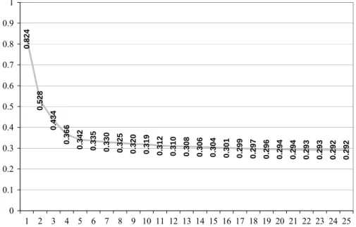
procedures on vegetation mask for noise removal...42 Figure 3.7 Reduction of Wilk’s lambda statistic for a single stepwise discriminant run
of CAN vs. RRP. The line begins to plateau at iteration 6 (delta <0.01) and
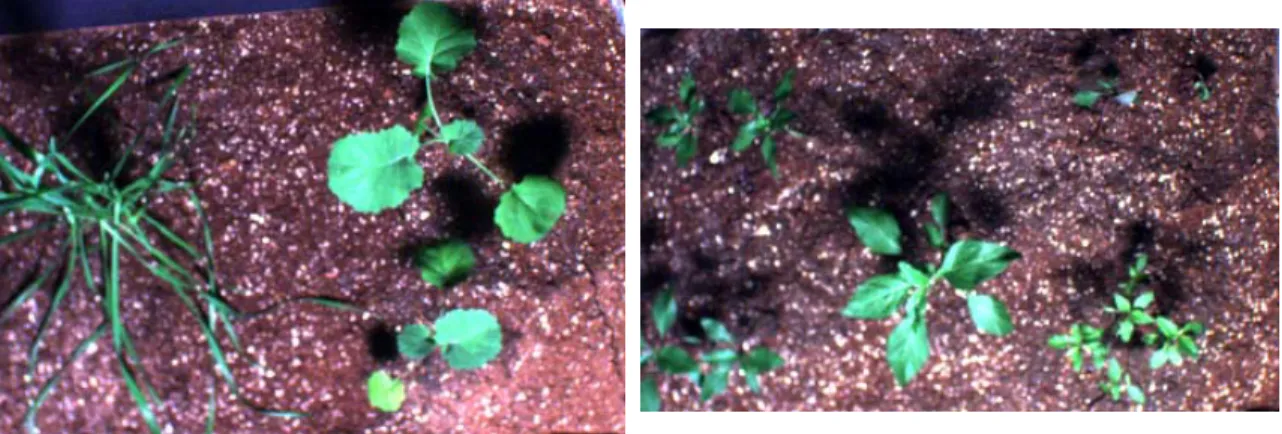
iteration 9 (delta <0.005). ...48 Figure 4.1 Laboratory acquired WHT and CAN (left) and RRP (right) image data
used for testing segmentation procedures...53 Figure 4.2 Processing steps in creation of vegetation mask for both WHT/CAN and
RRP treatments: (a) hue colour component; (b) 90-160° threshold image; (c) the result of the erode and dilate operators. ...55 Figure 4.3 Watershed segmentation results of WHT/CAN and RRP treatments on: (a)
8-bit; (b) 4-bit; (c) 3-bit hue bands. ...57 Figure 4.4 MCARI threshold technique for segmenting vegetation ((a) CAN/RRP and
(d) WHT/RRP) from background. MCARI vegetation index is calculated (b,e) and a value of 1 was applied to all pixels with a value of > 0.1 to create a mask of only vegetation pixels (c, f). ...59 Figure 4.5 Mean reflectance of crop (CAN=orange, PEA=green, WHT=cyan) and
weed (RRP=red, WO=blue) classes drawn from July 19 training data (Dotted
Figure 4.6 Mean reflectance of crop (CAN=orange, PEA=green, WHT=cyan) and weed (RRP=red, WO=blue) classes drawn from July 26 training data (Dotted
Lines = ±1 Standard Deviation)...62 Figure 4.7 ANOVA probability values (over 20 repetitions) plotted by waveband for
crop/weed combinations on July 19 acquisition date. Grey sections indicate wavelengths where no significant difference exists between weed/crop
combinations...64 Figure 4.8 ANOVA probability values (over 20 repetitions) plotted by waveband for
crop/weed combinations on July 26 acquisition date. Grey sections indicate wavelengths where no significant difference exists between weed/crop
combinations...65 Figure 4.9 Count of selected discriminatory bands (over 20 repetitions) plotted by
waveband for crop/RRP combinations on July 19 acquisition date. Black bars represent delta Wilk’s lambda 0.01; white bars represent delta Wilk’s lambda
0.005...67 Figure 4.10 Count of selected discriminatory bands (over 20 repetitions) plotted by
waveband for crop/WO combinations on July 19 acquisition date. Black bars represent delta Wilk’s lambda 0.01; white bars represent delta Wilk’s lambda
0.005...68 Figure 4.11 Percent contribution of original wavebands to PCA components C1 (solid
black), C2 (dashed black) and C3 (dashed grey) of first 5 repetitions for crop/weed combinations on July 19 acquisition date. The % of total variance accounted for by each C (average of 5 repetitions) is shown with cumulative
variance for each weed/crop combination. ...70 Figure 4.12 Single date MLC classification output of PEA (green) and RRP (red) on
(a) July 19 and (b) July 26 image data...73 Figure 4.13 MLC (b,e) and ANN (c,f) classification output of July 19 CAN (yellow)
(a,b,c)/RRP (red) (d,e,f) treatment. ...76 Figure 4.14 MLC (b,e) and ANN (c,f) classification output of July 19 WHT (cyan)
(a,b,c)/RRP (red) (d,e,f) treatment. ...76 Figure 4.15 MLC (b,e) and ANN (c,f) classification output of July 19 PEA (green)
(a,b,c)/WO (orange) (d,e,f) treatment. ...77 Figure 4.16 MLC (b,e) and ANN (c,f) classification output of July 26 CAN (yellow)
(a,b,c)/WO (orange) (d,e,f) treatment. ...77 Figure 4.17 Multitemporal MLC classification output of crop (PEA=green,
Figure 4.18 Multitemporal ANN classification output of crop (CAN=canola, PEA=green, WHT=cyan) and weed (RRP=red, WO=orange) combinations
acquired on July 19. ...80 Figure 4.19 MLC (a,b,c,d) and ANN (e,f,g,h) reduced waveband classification output
of crop (CAN=yellow, WHT=cyan, PEA=green) and weed (RRP=red,
LIST OF TABLES
Table 3.1 Planting depth and seed placement for greenhouse reared crop and weed
mixtures...36 Table 3.2 Seeding procedures for the field trials. ...37 Table 3.3 Crop (canola, pea and wheat) and weed (redroot pigweed and wild oat)
treatments designated for laboratory and field plot experiments...38 Table 3.4 Planting dates for crop/weed plots in 2005 field season...38 Table 3.5 Manually defined ROIs for both image acquisition dates. ...43 Table 3.6 Total number of ROIs and their associated pixels for each weed and crop
species investigated...44 Table 3.7 Number of ROI training samples and associated pixels selected for
classification training. Subset pixels selected by 1 of n sampling...45 Table 3.8 Pixels used for validation of field plot classification output. ...46 Table 4.1 MLC classification accuracy assessment with 61 wavebands input to
classification for (a) July 19 and (b) July 26 image acquisitions...74 Table 4.2 ANN classification accuracy assessment with 61 bands input to
classification for (a) July 19 and (b) July 26 image acquisitions...75 Table 4.3 Classification accuracy assessment for multitemporal classifications of
MLC for (a) July 19 and (b) July 26...79 Table 4.4 Classification accuracy assessment for ANNs multitemporal classifications
for (a) July 19 and (b) July 26...81 Table 4.5 Crop/weed (July 19 only) classification accuracy assessment for the
CHAPTER 1 INTRODUCTION
Precision agricultural techniques aim to manage fields based on spatial variability rather than generalized surveyed boundaries. With the rapid development of spatial mapping technologies, these techniques have now become a reality. Agricultural fields are typically non-uniform as spatial variability in soil properties and topography exists within field boundaries. Through gathering and maintaining information about this spatial variability, management of agricultural inputs including fertilizer, irrigation and pesticides can be applied at varied rates to promote efficient use and optimize crop production (Mulla and Schepers, 1997).
Site-specific herbicide management (SSHM) is one facet of precision agriculture, where herbicide application is dependant upon zones of weed density within the field rather than full spatial coverage application (Thompson et al., 1991). For weed
management, producers have three main options; mechanical control, chemical control or a combination of the two. Mechanical control involving tillage, with the exception of inter-row cultivation, is generally limited to pre-seeding or post-harvest situations in cropping operations. Research has linked tillage to soil erosion, the loss of soil moisture, and the spread of weed patches to other areas of the field (Brown and Steckler, 1995). With chemical management, a sprayer is typically used to apply a uniform amount of herbicide across the entire field. Because weeds tend to grow in patches and re-occur in the same areas each growing season (Mortensen et al., 1995; Tang et al., 1999; Martin-Chefson et al., 1999), a uniform application of herbicide may not yield optimal results in terms of economic efficiency.
SSHM allows for selective herbicide application based on zones of weed density and may result in a 30-72% reduction in herbicide requirements (Mortensen et al., 1995), thus increasing production profitability (Medlin et al., 2000). With reported Canadian pest control product sales totalling $1.34 billion (78% of which were herbicide) in 2005 (Crop Life, 2007), more efficient weed control practices could constitute a substantial savings to producers. Secondarily, SSHM techniques also reduce environmental
contamination potential, in terms of leaching to groundwater and losses to the atmosphere (Lindquist et al., 1998; Lippert and Wolak, 1999; Smith and Blackshaw, 2003).
Effective implementation of SSHM techniques requires detailed spatial information on the location and population density of weed species at the field scale. This information is costly and time consuming when acquired through traditional field survey techniques. Advances in spatial information technologies, including Global Positioning Systems (GPS), Geographic Information Systems (GIS) and Remote Sensing (RS) are offering land managers new tools for locating and targeting weed infestations (Swinton, 2005).
Passive optical remote sensing technology, which samples the reflected solar electromagnetic (EM) radiation over a specific area or picture element (pixel), provides information about targets of interest (ie. weed and crop species) from which reflectance features and spatial objects can be extracted. Differences in these measured
characteristics can then be used to create generalized classes (classification) over
agricultural fields. Investigations into the use of RS image data (ground-based, airborne and satellite) for the detection and mapping of weed infestations have provided
encouraging results (Tian et al., 1999; Bechdol et al., 2000; Tang et al., 2000; Radhkrishnan et al., 2002), as reviewed in Chapter 2.
SSHM systems can be separated into two main categories based on how the RS data are acquired and processed. The first is a system where a weed map is produced from satellite or airborne RS data acquired prior to herbicide application. A GIS
integrated with the sprayer would then selectively activate the spray nozzles based on the prescribed map locations. This technique would allow not only weed location and density to be used, but additional information including past yield, soil type and organic matter content could also be integrated into making the spray decision (Brown and Steckler, 1995). The main limitations to this type of system are the timely acquisition of image data and associated cost of tasking airborne and satellite missions.
These limitations can be mitigated through integration of the sensor, processing system and sprayer on the same implement in the field, which can then operate in real-time. As a producer navigates the field, the onboard sensor would acquire image data, process these data into weed location/density information and a resulting weed
prescription map would be interpreted with the herbicide being applied “on the fly” only in required areas. The very high spatial resolution of image data acquired (mm scale) at ground level increases potential to detect not only spectral differences between weed and crop species but also spatial differences in leaf shape and orientation. Challenges to this type of system include computational load of onboard processing and the requirement for efficient and accurate implementation of automated weed detection procedures (Tang et al., 1999).
This study investigated the image acquisition and processing component for a real-time SSHM system, and developed a procedure for the detection of select weed species in crops during the optimal herbicide application timeframe. A prototype camera system was used to acquire very high spatial (mm scale) and spectral (10 nm wavebands) image data over weed and crop treatments in both laboratory and field-based trials. The spectral and spatial resolution of image data acquired enabled testing the capability of both leaf shape and reflectance characteristics for discrimination of crop and weed species. Two classification techniques were evaluated for species discrimination: Artificial Neural Networks (ANNs) and Maximum Likelihood Classification (MLC). This initial detection step is required for subsequent mapping of weed location and prescribed locations for herbicide application.
Research objectives were to:
(a) evaluate the potential of very high spatial resolution image data for segmentation
of individual leaves and separation of background (soil, litter) from vegetation,
(b) identify the spectral characteristics from lab and field-based image data for use in
weed/crop differentiation,
(c) evaluate two supervised classification techniques (MLC and ANN) for accuracy
in species recognition and determine if a full hyperspectral dataset is required or a reduced number of bands are sufficient in classifying these data and
(d) characterize the effect of plant stage on spectral reflectance characteristics, and if
this variability can be accounted for in the classification procedures developed. Investigation into spectral and spatial differentiation of weed and crop species is required for development of SSHM techniques which are practical to the agricultural producer. The following chapter reviews the state of the art with respect to species discrimination using spectral and spatial characteristics and the use of image processing
techniques including segmentation and pixel-based classifiers for identification of weed/crop species, a preliminary step in the production of herbicide prescription maps.
CHAPTER 2 LITERATURE REVIEW
2.1 Introduction
Implementation of SSHM techniques requires knowledge of the location and density of weed species to make subsequent herbicide application decisions. This chapter identifies the spectral and spatial characteristics which have been used in discrimination of plant species. Acquisition of RS image data and the image processing procedures used for defining these spectral and spatial characteristics are explained and examples of weed and crop discrimination, drawn from published literature, are presented.
2.2 Vegetation Species Differentiation
Characteristic feature differences must exist between vegetated species for
accurate identification. The relationship of plant matter to incoming solar radiation is one feature which can be utilized to discriminate plant species. The plant tissue relationship to Electro-Magnetic (EM) radiation (reflectance and absorbance) is termed spectral signature, which is a measure of the reflectance properties of a target over a range of wavelengths (Figure 2.1).
0% 10% 20% 30% 40% 50% 60% 400 450 500 550 600 650 700 750 800 850 900 950 1000 Wavelength (nm) Re fle cta n ce Vegetation
Soil (Dark-Brown Chernozem)
Figure 2.1 Typical reflectance curves for soil and vegetation from field data acquired July 19, 2005.
Spectral signatures of photosynthetic plant species are similar with several characteristic absorption features caused by photosynthetically active material and internal leaf structure. Absorption features occur in the spectral range of 400-2500 nm due to photosynthetic pigments (450 and 670 nm) and water (970, 1200, 1450, 1950 and 2400 nm) (Gausman et al., 1973; Lillesand and Keifer, 1987; Grant, 1987; Curran, 1989; Vrindts et al., 1999; Lamb, 2000). The magnitude of these spectral responses is a
function of leaf thickness/structure, chlorophyll and other pigment concentrations and water content within the plant leaf (Lillisand and Keifer, 1987; Carter, 1991).
Chlorophyll and water content varies by plant species due to differences in physiology, and the ability to detect these variations using spectral response curves (signatures) is evident (Gausman et al., 1973; Lamb et al., 1999). This variability in spectral reflectance at specific wavelength regions of the EM spectrum, particularly in the visible and near-infrared (NIR), suggests potential for differentiation of weed from crop species
(Zwiggelaar, 1998).
Use of not only spectral characteristics but also spatial characteristics such as leaf shape and structural differences may also be used to identify and discriminate plant species. For example, monocotyledon species characterized by long narrow grass-like leaves are very different from the broad and circular leaves in dicotyledons. Through investigation of leaf shape measurements (perimeter, area, roundness etc.), different plant species could be identified based on spatial characteristics.
Given these spectral and spatial characteristics identified as important for species discrimination, RS technology is a valuable resource as it can provide both spectral and spatial information of selected targets on the ground. The following section describes the process by which RS data are acquired and how information can be extracted and applied to plant species discrimination.
2.3 Information from Remote Sensing Techniques
RS is the process by which data are recorded about an object, area or phenomenon by a sensor that is not in direct contact with that object, area or phenomenon (Lillisand and Kiefer, 1987). In this study, RS refers to the measurement and subsequent recording of reflected EM radiation at wavelengths from the visible (400-700 nm) to near-infrared (700-1000 nm) regions as provided by the sensor system utilized. The spectral, spatial
and temporal resolution of the RS data are of particular importance as these resolutions have a significant effect on the processing methods used and the information that can be extracted.
Spectral resolution refers to the measurement width (wavelength) and number of wavebands recorded in the RS data. A multispectral dataset will contain less than 10 relatively wide (~60-100 nm) wavebands, while a hyperspectal dataset can have 200 or more narrow wavebands (~1-20 nm) and typically are contiguous (ie. uninterrupted across the measured spectrum). The spatial resolution or scale of RS data refers to the area that each picture element (pixel) in the image represents on the ground. This is a function of the system optics and the platform on which the sensor is situated. For a given sensor configuration, greater target to sensor distance results in a larger ground area represented by a single pixel and therefore a lower spatial resolution. Generally, a sensor placed on a satellite platform will have lower spatial resolution than an airborne system, with the highest spatial resolution (mm scale) obtained using ground-based systems. Temporal resolution is simply the number of RS data acquisitions over time.
Data processing techniques are used to derive information about objects and areas of interest from the RS data. These processing tasks used in characterizing spectral and spatial differences, particularly in relation to weed and crop species discrimination are described in the following sections.
2.3.1Spatial Characteristics
The very high spatial resolution of ground-based sensors provides an opportunity for species discrimination based on leaf shape and textural features (Rosin, 2003; Cho et al., 2002). The majority of past studies utilized multispectral colour (Red, Green, Blue)
(RGB) charge-coupled device (CCD) sensor systems, as access to hyperspectral systems was limited. Defining leaf shape requires identification of foreground regions (plant pixels) and elimination of background features (soil and litter pixels) (Martin-Chefson et al., 1999). Foreground vegetation pixels can then be isolated using threshold techniques. Alternatively, processing methods such as watershed segmentation exist for identification of not only plant pixels but defining individual plant leaf segments.
2.3.1.1Image Thresholding
Thresholding is a common image processing technique to generalize image data and segment objects of interest based on the magnitude of spectral response. This procedure involves selection of the upper and lower range of pixel values for the object of interest (foreground pixels) and assigning them a single value, segmenting the image data into two classes, foreground and background. A transformation of RGB image data to Hue, Saturation and Intensity (HSI) colour space is a common practice to alleviate the effects of variable illumination (Cheng et al., 2001; Burks et al., 2000a) and typically provides better segmentation results.
Tang et al. (2000) reported a method for segmenting plant matter from background using a genetic algorithm based on HSI. The genetic algorithm is an adaptive search method modelled after the genetic evolutionary process. The algorithm searched for the best three-dimensional threshold boundaries in HSI colour space, which represented foreground (plant matter) in an image. This family of algorithms was highly efficient in search problems and was rarely affected by local minima due to the parallel exploration of the search space. The study utilized a colour CCD camera (Sony XC-003)
conditions. Similar results were obtained between algorithm output and manually
segmented images and the authors suggested this method could be used as a first step in a weed detection procedure to account for variable illumination conditions.
Another proposed method for recognizing plant species included both spectral and leaf geometric features used in a classification scheme (Chapron et al., 1999). Imagery
obtained over corn (Zea mays L.) and weed plots using a four band (RGB and NIR) CCD
camera (bandwidths and model not reported) were segmented into green plant matter and soil background using a series of Legendre filters (to remove signal noise) and thresholds of colour transformations. Colour transformations included HSI, and the Commission International de l’Eclairage colour space developed for perceptual uniformity (Cheng et al., 2001). The resulting image was classified into two classes (corn, not corn) using an expert system involving morphological filters that identified leaf shape. The procedure was robust under different illumination conditions but leaf overlap in the imagery hindered the classification accuracy, as the model could not efficiently separate overlapping leaves.
The calculation of texture statistics from HSI colour space has also shown promise in discrimination of weed species. Burks et al. (2000b) used an image analysis technique based on a Colour Co-occurrence Method (CCM) to discriminate five
greenhouse grown weed species [large crabgrass (Digitaria sanguinalis Scop.), giant
foxtail (Setaria faberi Herrm.), common lambsquarters (Chenopodium album L.), ivyleaf
morning-glory (Ipomoea hederacea (L.) Jacq.), velvetleaf (Abutilion theophrasti
Medicus)] and soil. The method involved colour transformation of RGB imagery (acquired with a colour CCD JVC TK-870U camera system) to HSI co-ordinates
followed by CCM matrix generation on the HSI bands, and Discriminant Analysis (DA) classification. To reduce the dimensionality of the CCM texture statistics (33 for each of the HSI matrices) and select layers that best identified textural differences between species, the authors used a Stepwise Discriminant Analysis (SDA). Overall classification accuracy was 93% for all six ground cover classes using 11 CCM texture features. The selected texture features used in the classification scheme did not include the intensity component thus reducing the processing time by one third and offering greater potential for a real-time herbicide application system.
2.3.1.2Watershed Segmentation
Watershed segmentation is a technique for identifying plant leaf segments within image data. Once defined, leaf shape differences can be used for species discrimination. This technique considers a grey scale image as a topographic surface with pixel values as “elevations”. Low points or minima on the surface are identified and the surface is flooded from these points. Building a “dam” keeps water from flowing between basins as flooded areas meet. Once the surface is completely flooded, watershed lines
represented by dams define regions in the image (Vincent and Soille, 1991; Beucher, 1992; Bleau and Leon, 2000; Rambabu et al., 2004).
Since its introduction by Beucher and Lantuejoul (1979), many researchers have published alterations to the algorithm to improve efficiency. The method developed by Vincent and Soille (1991) significantly reduced computational requirements for
segmentation and has made watershed segmentation an operational tool for practical use (Li et al., 1999). Though watershed segmentation has not been applied to leaf object
identification, it has been utilized to segment plant pixels from background (soil) in colour image data (Soille, 2000) using the red-green feature space.
2.3.1.3Leaf Shape Extraction
Once plant pixels are identified within the image through thresholding or other segmentation procedures, leaf shape measurements can be extracted. These can include, but are not restricted to, measurements of perimeter, area, aspect, roundness, compactness and elongation (Cho et al., 2002). Aitkenhead et al. (2003) obtained overall classification
accuracies of 62 to 67% in the identification of ryegrass (Lolium perenne L.) and fat hen
(Chenopodium album L.) in Autumn King carrot (Daucus carota L.) crops through a
single shape measurement (perimeter2/area). Using three shape features
(perimeter/broadness, elongation and aspect ratio) produced class accuracies of 92% for
radish (Raphanussativus L.) and 98% for an amalgamated weed class [purslane
(Portulaca oleracea L.), crabgrass and goosefoot (Chenopodium album L.)] (Cho et al.,
2002). Limitations to segmentation procedures for discrimination of crops and weeds based on leaf shape characteristics include size/stage of plant, leaf occlusion and shadow effects (Chapron et al., 1999; Brown and Noble, 2005).
2.3.2Spectral Characteristics
RS data can be used to derive information about the spectral characteristics of vegetated species. Classification is an image processing technique used to generalize complex image data into more meaningful categories or classes based on similarities in spectral pixel values. Different methods exist including statistical classifiers that group pixels based on clusters formed in the spectral domain. Artificial intelligence methods
such as ANNs, which attempt to model biological neural function, have been used in image classification and are shown to provide accurate and computationally efficient results (Atkinson and Tatnall, 1997). Studies involving the detection of weeds in agricultural cropping systems using pixel-based classification techniques are abundant (reviews by Lamb and Brown, 2001; Noble et al., 2002), and can be applied to RS image data of any spatial and/or spectral resolution. The following sections review statistical classifiers for detection of weeds in agricultural crops, followed by application of ANNs to crop/weed discrimination.
2.3.3Statistical Classifiers
2.3.3.1Airborne Sensing
Research into the creation of weed maps at the field scale using multi- and hyperspectral airborne remote sensing systems has been an active field of study (Brown et al., 1997; Lamb and Weedon, 1998; Medlin et al., 2000). Though limitations exist for spatial resolution, these systems are well suited to large area mapping and can provide information on weed location at the field level but not at the individual plant level.
Lamb and Weedon (1998) mapped panicgrass (Panicum effusum R. Br.) in canola
(Brassica napus L.) stubble using MLC and Normalized Difference Vegetation Index
(NDVI) thresholding. A four band CCD airborne system acquired spectral information over the blue (440 nm), green (550 nm), red (650 nm) and near-infrared (770 nm) regions of the electromagnetic spectrum at a spatial resolution of 1 m. The separation of green plant matter from soil and stubble background resulted in an overall classification accuracy of >87% for both MLC and NDVI threshold methods. Brown and Steckler
Beauv.), quackgrass (Agropyron repens (L.) Beauv.), dandelion (Taraxacum officinale
Weber) and lambsquarters in two no-till corn fields using MLC on both colour and colour-infrared photography (10 cm spatial resolution). Confusion between dandelion and lambsquarters was observed and these two classes were grouped. Species
differentiation was obtained in this study with an overall accuracy of 75%.
Medlin et al. (2000) used a four band CCD airborne system with one green (535-545 nm), two red (690-700 nm and 715-725 nm) and a NIR (835-845 nm) band, to acquire data over two early season (eight weeks post-seeding) soybean fields. The spectral response was linked to ground-based density populations of three weed species
[pitted morning-glory (Ipomoea lacunose L.), sicklepod (Senna obtusifolia (L.) Irwin &
Barnaby) and horsenettle (Solanum carolinense L.)]. The relationship between the
spectral response and weed density was tested through SDA. The imagery was classified using DA for the presence or absence of weeds rather than each weed species. A positive relationship between weed density and classification accuracy was established but
differentiation of weed species was not successful.
Few studies have tested the potential for species discrimination and weed map production using high spectral resolution airborne hyperspectral image data. Bechdol et al., (2000) acquired hyperspectral data using the Airborne Imaging Spectroradiometer for Applications system (SPECIM, Oulu, Finland), which records data over the spectral range of 450 to 900 nm. Images of three spatial resolutions (1, 2 and 3 m) were acquired over corn and soybean fields infested with eight weed species. The imagery was
atmospherically corrected and converted to reflectance. Through classification of minimum noise fraction feature space, weed infestation zones showed agreement with
ground-data collected over all spatial resolutions. Discrimination amongst weed species was not achieved.
2.3.3.2Ground-Based Sensing
Ground-based sensing platforms offer many advantages over airborne or satellite systems. These include absence of atmospheric scattering/absorption and very fine spatial resolution as the target is situated closer to the sensing system. A major limitation is spatial coverage, but in precision agricultural techniques aimed at individual fields, data are not required for large areas. Several methods have been developed for weed detection using statistical classifiers at ground level, using both multi- and hyperspectral image data.
An inexpensive CCD camera (Canon model 760) was utilized by Brown and Steckler (1993) to collect spectra (440, 530, 650, 730 nm) over a no-till corn field with
two weed species [quackgrass and milkweed (Asclepias syriaca L.)]. Image data were
acquired at 8 m as well as 600 m (aerial) above the target resulting in spatial resolutions of 15 and 150 mm respectively. Using MLC, >80% overall accuracy was obtained with the 600 m acquisition when defining three classes (weeds, corn and background) though individual weed species could not be differentiated. The 8 m acquisition enabled
separation of individual species as 66% of corn, 90% of quackgrass and 100% of
milkweed pixels were correctly classified. A similar project was reported (Brown et al., 1994) using the same sensing system and imaging techniques to acquire data over no-till corn with seven weed species. Again, MLC was used with optimal results obtained when weed species were joined into a single class.
Because many weeds can be characterised by red stems, El-Faki et al. (2000a, b) attempted to differentiate crop and weed species based on stem colour. Off nadir image data (45° incident angle) were collected using a colour CCD video camera (Sony XC-711) and provided a detailed view (mm spatial resolution) of the plant stems. Imagery was collected over trays of plants grown in a greenhouse. Trays included hard red winter
wheat infested with wild buckwheat (Polygonum convolvulus L.), cheat grass (Bromus
secalinus L.) and field bindweed (Convolvulus arvensis L.) as well as soybean infested
with johnsongrass (Sorghum halepense (L.) Pers.), redroot pigweed (Amaranthus
retroflexus L.) and yellow foxtail (Setaria glauca (L.) Beauv.). The method involved
testing both DA and ANNs for classification. A pre-processing step masked plant leaves, with the remaining stems passed to the classifications (DA, ANN). Mis-classification rates for most weed species were below 3% for both methods, with the DA producing the highest accuracy in crop classification (least square means of 55% for soybean and 62% for wheat). The authors stated that crop and weed stage were factors affecting the accuracy of weed detection.
Though ground-based hyperspectral imaging systems are rare, spectroradiometers which acquire spectral response of a single area (similar to a single pixel) provide the opportunity to measure reflectance characteristics of crop and weed species at very high spectral resolution and have provided encouraging results in weed detection and species discrimination studies. Vrindts et al. (2002) used an optical spectrum analyzer (Macam Photometrics Ltd., Livingston, Scotland) to obtain lab spectra from 400-2000 nm of seven weed species as well as corn and soybean. Through SDA, band ratios were selected that were deemed best for species discrimination. DA of these band ratios
produced classifications in which 97% of the weed and crop lab spectra were correctly classified. In the field, spectra from 400-900 nm were obtained using an Imspector V9 spectrograph (SPECIM). Using the same DA method, 90% of the crop and weed spectra were correctly classified. Illumination was a limitation as the discriminant models were developed under specific light conditions.
DA classification provided good results in a study of excised leaves of two crop (canola and spring wheat) and five weed species (lambsquarters, green foxtail, redroot
pigweed, wild mustard (Sinapis arvensis L.) and wild oat (Avena fatua L.)) (Smith and
Blackshaw, 2003). An ASD fieldspec pro spectroradiometer (Analytical Spectral Devices Inc., Boulder, CO.) and an LI-1800 integrating sphere (Li-COR Inc., Lincoln, Nebraska) were used to obtain spectra. Spectral resolution of these data were resampled to
hyperspectral (350-2500 nm at 10 nm intervals) and multispectral (representing the Landsat wavebands) datasets. Species classification accuracies of 89% and 90% were obtained using the multispectral and hyperspectral datasets, respectively. The authors suggested that the hyperspectral dataset was optimal as confusion was only observed within the monocotyledon species, whereas confusion between monocotyledon and dicotyledon species sometimes occurred in classification of the multispectral dataset.
An imaging spectrometer used by Borregaard et al. (2000) provided data for an extensive study of weed discrimination techniques including linear and quadratic DA, Principal Component Analysis (PCA) and partial least-squares regression. Using both visible (400-700 nm) and NIR (660-1060 nm) line imaging spectrometers (VTT
Electronics, Oulu, Finland), spectral data were acquired for two crops [sugar beet (Beta
bindweed and fools parsley (Aethusa cynapium L.). The imagery was segmented to
obtain pure plant spectra used in classification method evaluations. The bi-linear methods proved to be the most efficient with overall accuracies of 70-80% on four species (one crop and three weeds), and 90% when aggregated into two classes (crop and weed).
2.3.4Artificial Neural Networks
With the advancement of computing capability and the substantial amount of data supplied by imaging sensors, there is an increasing need for efficient data processing and interpretation tools. Artificial neural networks, which attempt to model biological neural pathways, have been used extensively in many different applications. The acceptance of ANNs in the field of remote sensing is due to several factors including the ability to handle complex feature space, to be computationally efficient and, to integrate different types of data (Atkinson and Tatnall, 1997). ANNs are also advantageous in that they can handle classes with two or more clusters in spectral space (i.e. aggregated class “soil” which contains both “bare soil” and “crop litter” pixels) and as a non-parametric approach, they do not have underlying assumptions such as multivariate Gaussian
normality (as in MLC). For classification of plant reflectance spectra, which are typically not normally distributed (Noble and Crowe, 2005), ANNs may present an advantage over more traditional techniques.
ANN development began with the introduction of the perceptron (Rosenblatt, 1958), a very simple feed-forward network model used to solve linear problems.
Network models were incapable of distinguishing classes that were not linearly separable until the mid-1980’s with the development of back-propagation training (Smith, 1993).
Through the past 40+ years, advancement in network architecture, training methodology and software design have resulted in the introduction of many ANN types, the most common being the feed-forward Multi-Layer Perceptron (MLP) trained by the back-propagation algorithm (Atkinson and Tatnall, 1997; Kannellopoulos and Wilkinson, 1997).
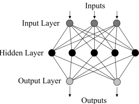
The MLP network consists of three or more layers including an input layer, one or more hidden layers and an output layer (Figure 2.2). Each layer contains a number of nodes which model biological neurons assembled by weighted channels creating a network. Input values are passed to the hidden layer with associated weights assigned to the connecting pathways. In each neuron, the weighted sum of all pathways is calculated and a linear (typically “sigmoid”) transformation function is applied to model non-linear transfer effects. The value then passes to the output layer (or subsequent hidden layer(s)). The output layer can have one or more nodes, with values ranging from 0-1. Each class is assigned a specific output range, and the output value is classified
Inputs
Input Layer
Hidden Layer
Output Layer
Outputs
Figure 2.2 The Multi-Layer Perceptron (MLP) network architecture.
Training the feed-forward MLP network is commonly achieved through back-propagation. This supervised training method utilizes input and output pairs to compute an overall error for the entire network. This overall error is minimized through an error signal that is fed back through the network and alters the individual connection weights (Lawrence, 1994). By utilizing known input and output pairs, the weights are adjusted through several iterations (termed epochs) until the appropriate output is achieved and overall network error is minimized.
One issue with ANN use is that it can be difficult to build the network model properly to achieve optimal or near-optimal network architecture, especially given the number of input parameters involved. This complexity has been somewhat mitigated with the release of commercial neural network software packages that provide initial values for network specification although these values are highly dependent on the application.
Neural networks first appeared in the remote sensing literature in the late 1980’s (Key et al., 1989; Benediktsson et al., 1990), with application to weed-crop
discrimination appearing in the late 1990’s (Yang et al., 1998, 2000; Moshou et al., 2001). Ground-based imaging sensors present the classifier with vast amounts of target information in the spatial and/or spectral domains to which ANNs are particularly well suited. This is important in real-time image processing systems that require
computational efficiency. The following section reviews several studies in which ANNs were utilized for classification of weed species in agricultural cropping systems.
2.3.5ANN Classification of Weeds in Agriculture
Machine vision based weed detection techniques provide very high resolution spatial imagery but are lacking in spectral dimensionality. In these applications, shape characteristics of plant leaves are investigated for discriminating species, particularly broadleaf (dicotyledon) crops infested with grassy (monocotyledon) weeds. Studies utilizing ANNs for classification of single plant image subsets, texture (co-occurrence measures) and leaf shape measurements aim to overcome the limited spectral information of machine vision sensors through incorporation of spatial species differences (Cho et al., 2002; Aitkenhead et al., 2003; Yang et al., 2000 & 2003; Burks et al., 2000a & 2005).
ANN classification of six weed species based on 11 CCM texture measurements (Burks et al., 2000b) expanded on a previous texture study (Burks et al., 2000a). The network architecture was evaluated by altering the number of nodes in the two hidden layers. The network model produced consistently high classification accuracies with the best topology producing a 97% overall (approx 90% individual class) accuracy.
Testing different network architectures based on classification accuracy also suggested that a large network does not necessarily produce the highest accuracies. This study was extended to evaluate different network types including counter-propagation, back-propagation, radial basis function and the DA classifier (Burks et al., 2005). The authors suggested the importance of reducing the number of input variables using SDA as a consistently successful procedure for simplification of the classification problem. From the several classification methods utilized, the back-propagation network model produced the highest accuracy (97%).
Cho et al. (2002) proposed an approach for discrimination between radish and three weed species based on leaf measurements (area, perimeter, length, width and length of major and minor axes) used to calculate eight shape features (aspect ratio, roundness, compactness, elongation, perimeter to broadness ratio, length to perimeter ratio, length to width ratio and cube of perimeter to area by length ratio) input to a MLP network model. Vegetation was segmented from the acquired colour imagery using Photoshop (Adobe Systems Inc., San Jose, CA), and shape characteristics were extracted using Image Pro Plus (Media Cybernetics Inc., Silver Spring, MD). SDA was used to identify three shape measurements (perimeter/broadness, aspect and elongation) classified using DA, while all eight measurements were used as input to an ANN. A network architecture of eight input, seven hidden and two output nodes classified 10 radish and 20 weed images with 100% accuracy, while the DA classifier produced 93% and 94% class accuracy in radish and weeds, respectively.
Aitkenhead et al. (2003) used a MLP neural network for discrimination amongst crop (carrot), weeds (ryegrass and fat hen) and soil. Image pre-processing involved
delineating subset blocks of 32 x 24 pixels that contained plant matter. Two image
classification methods were tested. First, a shape characteristic (perimeter2/area) mean
was calculated from the training subset image data for the weed and crop classes and the validation blocks were classified based on distance to class means. Secondly, the image subsets identified were classified using an ANN with the whole image block passed to the input layer, two hidden layers and two output values (soil=0,0; carrot=1,0; weeds=0,1; crop and weeds=1,1). When plants of varied size were considered, the shape
characteristic produced a classification accuracy of 62%, while the ANN classified between 62-82% of plant sample images correctly.
The effects of feed-forward back-propagation network architecture on
classification of corn and seven weed species were evaluated in a study by Yang et al. (2000). Image data were collected using a Kodak DC50 RGB camera from which image subsets of 100 x 100 pixels containing a single crop or weed plant were manually
selected. The subsets were converted from 24-bit colour to 8-bit grey scale. Several ANN architectures were created using Neural Network Toolbox v.2.0 for Matlab v.5.0 (Mathworks, Natick, MA) in which a single hidden layer contained 70 to 300 nodes with one (crop=1; weeds=0) or two nodes (crop=1,0; weeds=0,1) in the output layer. It was expected that the network with two output nodes would give an estimate of probability and that this would give some flexibility to interpretation of results. The single output network produced class accuracies of 70-100% for corn and 50-80% for weeds while the network with two outputs produced accuracies of 60-90% for corn and 40-80% for weed classes. McNemar and Briar Score statistics showed no significant differences between the various network models based on their predictive abilities. This suggested the
simplest model (least hidden and output nodes) was as effective in crop/weed discrimination as the more complex model.
This study was later expanded to detect four weed species in corn (Yang et al., 2003). Subset images of single plants were again defined (60 x 60 pixels) and converted to grey scale with four orientations per image (0°, 90°, 180° and 270°). Two types (crop/amalgamated weed and crop/single weed) of ANNs were developed using NeuralWorks Professional II v5.23 (NeuralWare Inc., Pittsburgh, PA) with a single hidden layer of multiple nodes (100 – 1000) and one and two output nodes. The resulting networks produced accuracies of 54-90% for corn and 32-100% for single weed species. This performance range indicated the importance of sample size and network
architecture. Species type also affected classification accuracy as the worst classification accuracy was for corn and quackgrass, both of which are monocotyledon species and have similar leaf structural characteristics. Higher class accuracies were obtained for the crop/individual weed as opposed to the crop/amalgamated weed class.
Discrimination between sunflower (Helianthus annuus L.), common cocklebur
(Xanthium strumarium L.) and background using three band (RGB) ground-based image
classification with a MLP network using 1, 2 and 3 hidden layers was recently conducted (Kavdir, 2004). Network models developed consisted of sunflower-weed, plant-bare soil and sunflower-weed-soil classification schemes. The architectures consisted of 4800 inputs (3 colour values x 40 x 40 pixels) with 35-300 nodes in the first, 15-100 in the second and 7-15 in the third hidden layers.
The best classification for sunflower-weed scheme was obtained using three hidden layers (50 x 25 x 7) with 70 of 86 images correctly identified. Models with one or
two hidden layer architectures achieved slightly lower accuracies, though logistic
regression showed no statistically significant difference in networks with 1, 2 or 3 hidden layers in discriminating plant and soil. Classification of the sunflower-weed-soil scheme had 93 of 129 images correct with one hidden layer and 103 of 129 using models with two hidden layers. Again classification accuracy of the ANN models was highly sensitive to network architecture. Because shadow and variability in plant size were inherent in these image data the author suggested further work should focus on in-field experiments where soil type and crop residue may affect classification accuracies.
Few studies have addressed weed-crop discrimination with ANNs using ground-based hyperspectral data. As discussed in section 2.1, plant spectral reflectance
characteristics in bands outside the visible region of the electromagnetic spectrum provide more information than RGB colour imaging sensors and may increase the feasibility of weed-crop discrimination. Moshou et al. (2001) collected point spectra (200-2000 nm at 10 nm wavelengths) over corn, sugar beet and several weed species (individual species not identified). Discriminatory bands were selected from the 200 available using correlations between the two classes (high correlation indicates more information content contained within the band).
This procedure identified five bands for corn-weed and three bands for sugar beet-weed classifications. Different ANN types were tested including MLP trained using adaptive learning rate and momentum, Self-Organizing Map (SOM) trained with local linear mappings and, probability neural networks. The MLP classifier accuracies were 90% / 66% (corn / weed) and 86% / 94% (sugar beet/weed) but the best performance was observed in the SOM network with class accuracies of 96% / 90% (corn / weed) and 98%
/ 97% (sugar beet / weed). The authors suggested that the SOM network obtained faster convergence and produced better overall classification performance.
2.4 Summary
Research into the detection and discrimination of weeds in crops from both ground-based and aerial platform remote sensing systems is extensive. Spectral, spatial and temporal resolution often limits using aerial and satellite platform sensors for plant species discrimination and revisit schedules of satellite-based systems can hinder acquisition of data at critical plant stages (Radhkrishnan et al., 2002). Ground-based sensor systems are an attractive alternative due to the very high spatial resolution (mm scale) of image data but attention must be given to the increased computational cost of processing these data (Brown and Noble, 2005). Few studies have investigated the potential of hyperspectral image data for weed crop discrimination mainly due to lack of sensor system availability and higher cost.
Segmentation techniques, especially thresholding have consistently been applied for separation of foreground vegetation pixels from background in very high spatial resolution image data. This first step of segmentation can be used to define shape characteristics and also identify foreground pixels in RS image data. Identification of vegetation pixels can simplify the weed-crop classification problem through eliminating the need for soil or litter classes.
Building on past research, this study investigated the potential for weed and crop discrimination from the rich information (spectral and spatial) ground-based
methods used in acquisition and analysis of RS data for addressing the study objectives introduced in Chapter 1.
CHAPTER 3 MATERIALS AND METHODS
3.1 Introduction
This chapter describes equipment and procedures used in acquisition of
hyperspectral image data and its evaluation for detection of selected weed species in post-emergent crops. This is followed by radiometric correction and procedures for
conversion of raw image data to reflectance. The laboratory and field experimental design is presented followed by image segmentation techniques explored for identifying pixels of vegetation as well as identification of individual leaves within acquired image data. A method for selection of a subset of wavelengths, which are important for species discrimination, is presented as well as classification (MLC and ANN) techniques used to define species location within the image data. Validation methods for assessing
classification accuracy, important for comparison of the two classification procedures, are then explained.
3.2 Hyperspectral Imaging System
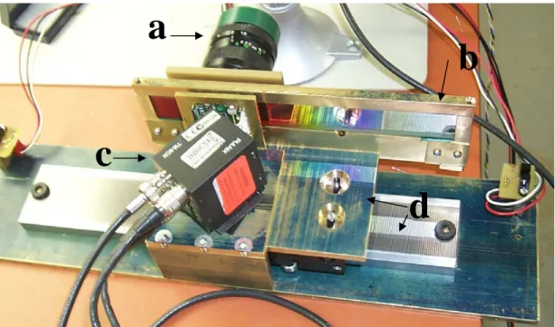
The hyperspectral imaging system (Figure 3.1) and image acquisition software were developed by DeltaTee Enterprises Ltd. located in Calgary, Alberta, Canada. The system uses a magnetic carriage to “step” a linear variable filter (Schott Veril, VIS-NIR 200) across a charge-coupled device (CCD) sensor for hyperspectral image acquisition. The interference filter’s central wavelength varies linearly over a 200 mm length of glass substrate (Figure 3.2) and permits acquisition of a data cube with 61 wavebands from 400 – 1000 nm at 10 nm increments. The imaging sensor, manufactured by Point Grey Research (Vancouver, British Columbia) uses a 0.5 inch progressive scan CCD sensor
(Sony, ICX414AL). This sensor outputs a 640 x 480 pixel image with a signal to noise ratio of greater than 60 dB. Image data output are 16-bit unsigned integers, enabling a raw digital number (DN) dynamic range of 0 – 65535. The system focuses incoming radiation with an 8 mm C-mount VIS-NIR lens (Schneider Kreuznach, Germany) fixed to create 44 º vertical and 33º horizontal fields-of-view with the focus and aperture (f/1.4 to f/11) adjusted manually. This range in aperture settings ensures the system can be set to avoid saturation (DN reading above the 65535 limit of the CCD).
The image acquisition software (SPDaq, DeltaTee Enterprises Ltd.) allows electronic shutter and waveband width adjustments, and was used to acquire, save and perform radiometric correction of the hyperspectral image data.
a
b
c
d
Figure 3.1 Hyperspectral imaging system components; a) lens, b) linear variable filter, c) imaging sensor and d) carriage system.
Figure 3.2 Linear relationship between measuring distance and wavelength in 200 mm filter (obtained from Edmund Optics, 2007).
3.3 Calibration of Image Data
Prior to image analysis, the acquired image data were radiometrically corrected. This consisted of three steps; dark correction, frequency resampling and uniformity correction. The final processing step, conversion to reflectance, was achieved using the ENVI/IDL software package (ITT Industries Inc., Boulder, CO). The following sub-sections discuss each correction applied.
3.3.1Dark Current Correction
Dark current correction accounts for internal signal noise and false response in the CCD potential wells inherent to this type of imaging system. Thermal energy read as incoming photons can constitute a false reading of incoming radiation termed dark noise. Dark noise is positively related to thermal energy, and as the temperature of the imaging environment changes, particular attention must be given to dark noise effects. Correction involved collection of 200 frames with the lens covered to eliminate all sources of
image of measured dark noise which was subtracted from each band in successive image acquisitions. Dark noise correction data were acquired regularly throughout the period of image data collection to account for variation in dark noise effects.
3.3.2Frequency Resampling
The raw image data consisted of several frames in which wavelength varied across the X dimension due to the linear variable filter used in the hyperspectral image acquisition. A frequency resampling technique applied to the data cube transformed these data into frames of one consistent wavelength. The procedure shifts the frequency data through a linear interpolation to adjacent images to produce a single wavelength horizontally across the image (Figure 3.3). A number of extra images are taken to avoid extrapolation. The factors for this correction (slope and intercept) are specific to the filter used in the imaging system and were calculated by the manufacturer.
Extra im ages Raw data Re-sampled data Wa v e le n g th Colum n
3.3.3Uniformity Correction
Uniformity or flat field correction reduces variability in the imaging scene caused by fluctuation of the quantum efficiency of each potential well in the CCD matrix, termed photo response non-uniformity. Secondly, as a result of circular lens optics, a gradient effect (viginetting) across the image is inherent in any imaging system. Uniformity correction, which corrects these effects, can be calculated by filling the field-of-view with a target of consistent reflectance. An integrating sphere was developed and used for uniformity coefficient collection at DeltaTee’s laboratories.
The camera was setup to view the evenly illuminated integrating sphere. For each f/stop the shutter speed was adjusted so that the maximum value in the dataset was
approximately 75% of the full dynamic range. With the optimal shutter speed
established, a full hyperspectral data cube was acquired and dark correction applied. The wavelength at which the highest signal response occurred was identified, and the average value was calculated for that band. A correction coefficient matrix was created by dividing the average value by the value for each pixel (Equation 3.1). Multiplication of this uniformity coefficient matrix with each band in the acquired hyperspectral data produces a uniformity corrected image. The coefficient matrix is calculated by:
y x y
x Avg U
C , = / , (3.1)
where Avg is the average DN value, Ux,y is the DN value of a pixel at column x and row
3.3.4Reflectance Conversion
The final step of image processing involved conversion of DN values to reflectance. Reflectance is a measure of the percentage of incoming solar radiation reflected by an image target on a per pixel basis. This conversion required imaging a Spectralon (polytetrafluoroethylene) calibration panel. The panel reflects approximately 99% of incoming solar radiation across the 400-1000 nm wavelength range of the
imaging system, with reflectance coefficients provided by the manufacturer (Labsphere, Inc., North Sutton, NH) at 50 nm increments (Appendix A).
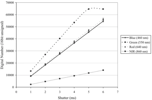
Immediately before and after image acquisition, the Spectralon panel was imaged (f/11 and shutter speed = 2-4 ms) ensuring sensor saturation did not occur. The raw image pixel values of the reference panel were extracted and band means calculated. Acquisition of laboratory and field plot data required a slower shutter speed to provide appropriate signal strength to the CCD sensor, and typically ranged from 4-8 ms. The relationship between exposure time and DN output in the CCD sensor system evaluated and found to be linear up to the saturation point (DN=65535) (Figure 3.4). This
suggested a conversion ratio could be applied prior to reflectance conversion, accounting for differences in shutter speed between the acquired panel and target image data.
0 10000 20000 30000 40000 50000 60000 70000 0 1 2 3 4 5 6 7 Shutter (ms) Dig ita l Num be r (16b it unsigne d) Blue (460 nm) Green (550 nm) Red (640 nm) NIR (860 nm)
Figure 3.4 Relationship between electronic shutter and raw digital numbers on CCD sensor (Mean n=4544, error bars = +/- standard deviation).
An IDL program was written to convert the image data cubes to reflectance (Equation 3.2). The program includes an exposure multiplier (conversion ratio), which accounts for instances where the reference panel was collected at a different shutter speed (same aperture) than the target/plot images. For example, if a panel image acquired at 2 ms is used to correct a field image acquired at 6 ms then the exposure multiplier would be 3. The program multiplies the DN’s of the calibration target by 3 before reflectance correction is run. Reflectance is calculated as:
R(x,y,b) = ( I(x,y,b) * SP(b)) / CT(b) (3.2)
where CT is the calibration target average DN, I is the image DN value, R is the image reflectance value, SP is the spectralon panel reflectance coefficient and x,y,b represent the horizontal coordinate, vertical coordinate and band, respectively.
3.4 Experimental Design
3.4.1Crop and Weed Species
It was important that the weed/crop species selected in the study represent both monocotyledon and dicotyledon morphologies encountered in agricultural applications, as well as being of economic importance in western Canadian cropping systems. Based
on these criteria, three crop species [Eclipse field pea (PEA) (Pisum sativum L.), Invigor
5020 canola (CAN) (Brassica napus L.), and AC Barrie spring wheat (WHT) (Triticum
aestivum L.)] and two weed species [redroot pigweed (RRP) (Amaranthusretroflexus L.)
and wild oat (WO) (Avenafatua L.)] were selected for investigation.
3.4.2Laboratory Trial
Using laboratory and greenhouse facilities located at the Agriculture and Agri-Food Canada Research Centre in Lethbridge, Alberta, weed/crop mixtures were seeded in trays of Cornell mix, an equal-part mixture of sphagnum peat moss and vermiculite (Table 3.1). These treatments were grown in a greenhouse under sodium vapour lighting with a 16 hour day - 8 hour night cycle at a constant temperature of 21° C.
Table 3.1 Planting depth and seed placement for greenhouse reared crop and weed mixtures.
Species Planting Depth (cm) Seed Placement
canola 1.5-2 0.5 cm spacing
pea 5 0.5-1cm spacing
wheat 4 Seed end to end
redroot pigweed
Surface Broadcast, and
raked into surface
wild oat 1.5-2 Broadcast, covered
Four replications of these treatments were planted at approximately two-week intervals. For this study, canola, redroot pigweed and a single wheat plant were transplanted into two trays. These trays provided a variety of leaf shapes and sizes, sufficient for initial testing of segmentation procedures.
3.4.3Field Trial
The field study site was located at the Agriculture and Agri-Food Canada Research Centre in Lethbridge, Alberta (49.7°N, 112.833°W). The soil type was Dark Brown Chernozemic of lacustrine origin with a pH of 8.0 and 3% organic matter content. Weeds were surface broadcast on plots (5 m x 2.5 m) prior to seeding the various crops (Table 3.2). Seeder movement over plots allowed the broadcast weeds to be embedded in
the soil, facilitating germination. During the seeding operation, nitrogen at 40 kg ha-1 and
phosphorous at 10 kg ha-1 were banded 10 cm deep between crop rows.
Table 3.2 Seeding procedures for the field trials.
Species Rate Depth
(cm) Row Spacing (cm) canola 8 kg ha-1 1-2 23 pea 253 kg ha-1 5 23 wheat 124 kg ha-1 4 23 redroot pigweed 27 g plot -1 Surface N/A
wild oat 100 g plot-1 Surface N/A
Field plots of the eleven treatments (5 monocultures and 6 weed/crop
combinations) (Table 3.3) were seeded on four dates (Table 3.4) to increase the window of opportunity for collecting timely (weather/crop stage) image data. Spring flooding hindered the first two seeding dates but hand watering of trial 3 and 4 improved