DOI 10.1007/s10994-006-5834-0
Propositionalization-based relational subgroup discovery
with RSD
Filip ˇZelezn´y·Nada Lavraˇc
Received: 24 February 2003 / Revised: 1 December 2004 / Accepted: 27 July 2005 / Published online: 27 January 2006
C
Springer Science+Business Media, Inc. 2006
Abstract Relational rule learning algorithms are typically designed to construct
classifi-cation and prediction rules. However, relational rule learning can be adapted also to sub-group discovery. This paper proposes a propositionalization approach to relational subsub-group discovery, achieved through appropriately adapting rule learning and first-order feature construction. The proposed approach was successfully applied to standard ILP problems (East-West trains, King-Rook-King chess endgame and mutagenicity prediction) and two real-life problems (analysis of telephone calls and traffic accident analysis).
Keywords Relational data mining . Propositionalization . Feature construction . Subgroup
discovery
1. Introduction
Classical rule learning algorithms are designed to construct classification and prediction rules (Michie et al.,1994; Clark & Niblett,1989; Cohen,1995). The goal of these predictive induction algorithms is to induce classification/prediction models consisting of a set of rules. On the other hand, opposed to model induction, descriptive induction algorithms (De Raedt & Dehaspe,1997; Wrobel & Dˇzeroski,1995) aim to discover patterns described in the form of individual rules. Descriptive induction algorithms include association rule learners (e.g., APRIORI (Agrawal et al.,1996)), clausal discovery systems (e.g., CLAUDIEN (De Raedt & Dehaspe,1997; De Raedt et al.,2001)), and subgroup discovery systems (e.g., MIDOS
Editors: Hendrik Blockeel, David Jensen and Stefan Kramer
F. ˇZelezn´y ()
Czech Technical University, Prague, Czech Republic e-mail: [email protected]
N. Lavraˇc
Institute Joˇzef Stefan, Ljubljana, Slovenia, and Nova Gorica Polytechnic, Nova Gorica, Slovenia e-mail: [email protected]
(Wrobel,1997; Wrobel,2001), EXPLORA (Kloesgen,1996) and SubgroupMiner (Kloesgen & May,2002)).
This paper investigates relational subgroup discovery. As in the MIDOS relational sub-group discovery system, a subsub-group discovery task is defined as follows: Given a population of individuals and a property of individuals we are interested in, find population subgroups that are statistically ‘most interesting’, e.g., are as large as possible and have the most unusual statistical (distributional) characteristics with respect to the property of interest.
Notice an important aspect of the above definition: there is a predefined property of interest, meaning that a subgroup discovery task aims at characterizing population subgroups of a given target class. This property indicates that standard classification rule learning algorithms could be used for solving the task. However, while the goal of classification rule learning is to generate models (sets of rules), inducing class descriptions in terms of properties occurring in the descriptions of training examples, in contrast, subgroup discovery aims at discovering individual patterns of interest (individual rules describing the target class).
This paper proposes to adapt classification rule learning to relational subgroup discov-ery, based on principles that employ the following main ingredients: propositionalization through first-order feature construction, feature filtering, incorporation of example weights into the weighted relative accuracy search heuristic, and implementation of the weighted covering algorithm. Most of the above-listed elements conform to the subgroup discov-ery methodology proposed by Lavraˇc et al. (2004); for completeness, these elements are described in Section3. The main contributions of this paper concern the transfer of this methodology to the multi-relational learning setting. The contributions include substan-tial improvements of the propositionalization step (compared to the propositionalization proposed by Flach and Lachiche (1999) and Lavraˇc and Flach (2001)) and an effective implementation of relational subgroup discovery algorithm RSD, employing language and evaluation constraints. Further contributions concern the analysis of the RSD subgroup dis-covery algorithm in the ROC space, and the successful application of RSD to standard ILP problems (East-West trains, King-Rook-King chess endgame and mutagenicity predic-tion) and two real-life problem domains (analysis of telephone calls and analysis of traffic accidents).
RSD is available at http://labe.felk.cvut.cz/∼zelezny/rsd/. This web page gives access to the RSD system, the user’s manual, the data sets (Trains, KRK, Mutagenesis, Telecom)1and the related parameter setting declarations, which enable the reproduction of
the experimental results of this paper.
The paper is organized as follows. Section2specifies the relational subgroup discovery task, illustrating first-order feature construction and results of rule induction on the well-known East-West challenge learning problem. It also defines criteria for evaluating the results of subgroup discovery algorithms. In Section3, the background of this work is explained, including pointers to the related work. Sections4 and5present the main ingredients of the RSD subgroup discovery algorithm: propositionalization through efficient first-order feature construction and constraint-based induction of subgroup descriptions, respectively. Section6describes the experimental domains. The results of experiments are presented in Sections7and8. Section9concludes by summarizing the results and presenting plans for further work.
Table 1 A subgroup description induced in the Trains domain and the list of definitions of features appearing as literals in the conjunctive antecedent of the rule. Definitions of features are described in the Prolog format
East(A)←f16(A)∧ ¬f69(A)∧ ¬f93(A) [10,1]
f16(A) :- hasCar(A,B), carShape(B,rectangle), carLength(B,short), hasSides(B,notDouble)
f69(A) :- hasCar(A,B), carShape(B,bucket), hasLoad(B,C), loadShape(C,circle)
f93(A) :- hasCar(A,B), carShape(B,rectangle), hasLoad(B,C), loadShape(C,circle),loadNum(C,3)
SubgroupTrains1for target classEastconsists of East-bound trains which have a short rectangle car without double-sides, do not have a bucket-shape car with a circle load, and do not have a rectangle car with three circle loads.
2. Relational subgroup discovery: Problem definition
In contrast with predictive induction algorithms which induce models in a rule set form, subgroup discovery aims at finding patterns in the data, described in the form of individual rules. This fact is reflected in the subgroup discovery task definition outlined below.
The input to the RSD relational subgroup discovery algorithm consists of a relational database (possibly deductive, further called the input data) containing (a) one main relation defined by a set of ground facts (training examples), each corresponding to a unique individual and having one argument specifying the class, (b) background knowledge in the form of a Prolog program (possibly including functions and recursive predicate definitions), and (c) syntactic and semantic constraints, defined for the purpose of first-order feature construction and constraint-based subgroup discovery.
The output of RSD is a set of individual rules, each describing a subgroup of individuals whose class distribution differs substantially from the class distribution in the input data set. The rule antecedents (bodies) are conjunctions of symbols of pre-generated first-order features.
The task of relational subgroup discovery is illustrated by a simple East-West trains learning problem, where the subgroup discovery task is to discover patterns in the form of Prolog clauses defining subgroups biased towards one of the two classes: East and West. The original learning task (Michie et al.,1994) was defined as a classification problem and not as a subgroup discovery problem.
Table1shows an example subgroup induced from a dataset consisting of 20 trains (10 East-bound and 10 West-bound), where subgroupTrains1is described in rule form H
←B [TP, FP]; rule head H denotes the target class, B is the rule body consisting of a conjunction of first-order features, and TP and FP denote the number of true positives (positive examples covered by the rule, correctly predicted as positives) and the number of false positives (negative example covered, incorrectly predicted as positives), respectively. Note that individual feature definitions contain a key variable corresponding to the given individual (the individual ‘train’). In evaluation, the truth value of a feature is determined with respect to the individual which instantiates the key variable.
RSD aims at discovering subgroups that are ‘most interesting’ according to predefined criteria used to measure the interestingness of a subgroup. We consider a subgroup to be interesting if it has a sufficiently large coverage and if it is sufficiently significant (i.e., if it has a sufficiently unusual class distribution compared to the entire training set). In addition, we define quality criteria on sets of subgroups. These are the averages of the coverage and
significance of the rule set, the rule set complexity and the area under the ROC convex hull formed by the best subgroups. Below we define the quality criteria for individual rules and rule sets.
Coverage. Coverage of a single rule Riis defined as
Cov(Ri)=Cov(H←Bi)= p(Bi)=
n(Bi)
N
where N is the number of all examples and n(Bi) is the number of examples for which the
conditions in body Bihold.
Average rule coverage measures the percentage of examples covered on average by one rule of the induced rule set. It is computed as
COV= 1 nR nR i=1 Cov(Ri)
where nRis the number of induced rules.
Complexity. Average rule complexity is measured by a pair of values R:F, where R stands
for the average number of rules/subgroups per class, and F stands for the average number of features per rule.
Significance. This quantity measures how significantly different the class distribution in a
subgroup is from the prior class distribution in the entire example set. We adopt here the significance measure used in the CN2 algorithm (Clark & Niblett,1989), where the significance of rule Riis measured in terms of the likelihood ratio statistic of the rule as
follows: Sig(Ri)=2· j n(Hj·Bi)·log n(Hj·Bi) n(Hj)·p(Bi) . (1)
where for each class Hj, n(Hj·Bi) denotes the number of instances of Hjin the set where
rule body Biholds, n(Hj) is the number of Hjinstances, and p(Bi) (i.e., rule coverage
computed as n(Bi)
N plays the role of a normalizing factor. Note that although for each
generated subgroup description one class is selected as the target class, the significance criterion measures the distributional unusualness unbiased to any particular class; as such, it measures the significance of the rule condition only.
Average rule significance, in a rule set consisting of nRrules, is computed as
S I G= 1 nR nR i=1 Sig(Ri).
Area under the ROC curve. Each rule (subgroup) is represented by its true positive rate
(TPr) and false positve rate (FPr)2 as a point in the ROC space, where the X-axis corresponds to FPr and the Y-axis to TPr. Plotting rules in the ROC space allows us to
2The sensitivity or true positive rate of rule H←B is computed as TPr= T P Pos = n(H·B) n(H ) , and FPr= F P N eg= n(H·B)
compare the quality of individual rules and select the set of best rules, located on the ROC convex hull. To evaluate a set of induced subgroup descriptions, the area under the ROC convex hull (the AUC value) of a set of best subgroup descriptions is computed. Subgroup evaluation in the ROC space is explained in detail in Section3.6.
3. Background and related work
This section provides pointers to related work and presents the background of the proposed approach to relational subgroup discovery.
3.1. Related subgroup discovery approaches
Well-known systems in the field of subgroup discovery are EXPLORA (Kloesgen,1996), MIDOS (Wrobel,1997,2001) and SubgroupMiner (Kloesgen & May,2002). EXPLORA treats the learning task as a single relation problem, i.e., all the data are assumed to be available in one table (relation), while MIDOS and SubgroupMiner perform subgroup discovery from multiple relational tables. The most important features of these systems, related to this paper, concern the definition of the learning task and the use of heuristics for subgroup discovery. The distinguishing feature of RSD compared to MIDOS and SubgroupMiner is that the latter two systems assume as input the tabular representation of training data and background relations. On the other hand, RSD input data has the form of ground Prolog facts and background knowledge is either in the form of facts or intensional rules, including functions and recursive predicate definitions.
Exception rule learning (Suzuki, 2004) also deals with finding interesting population subgroups. Recent approaches to subgroup discovery, SD (Gamberger and Lavraˇc,2002) and CN2-SD (Lavraˇc et al.,2004), aim at overcoming the problem of inappropriate bias of the standard covering algorithm. Like the RSD algorithm, they use a weighted covering algorithm and modify the search heuristic by example weights. SD and CN2-SD are propositional, while RSD is a relational subgroup discovery algorithm. The subgroup discovery component of RSD shares common basic principles with CN2-SD: the fundamental search strategy and the heuristic function employed therein (the weighted relative accuracy heuristic function is just slightly modified). RSD’s subgroup discovery component however implements additional features, such as constraint-based pruning (by detecting when the heuristic function cannot be improved via refinement of the currently explored search node) and various stopping criteria for rule search, employing user-specified constraints.
3.2. Related propositionalization approaches
Using relational background knowledge in the process of hypothesis construction is a dis-tinctive feature of relational data mining (Dˇzeroski & Lavraˇc, 2001) and inductive logic programming (ILP) (Muggleton,1992; Lavraˇc & Dˇzeroski,1994).
In propositional learning the idea of augmenting an existing set of attributes with new ones is known as constructive induction. The problem of feature construction has been studied extensively (Pagallo & Haussler,1990; Cohen & Singer,1991; Oliveira & Sangiovanni-Vincentelli,1992, Koller & Sahami,1996; Geibel & Wysotzki,1996). A first-order counter-part of constructive induction is predicate invention (see e.g., Stahl,1996for an overview of predicate invention in ILP).
Propositionalization (Lavraˇc & Dˇzeroski,1994; Kramer et al.,2001) is a special case of predicate invention enabling the representation change from a relational representation to a propositional one. It involves the construction of features from relational background knowledge and structural properties of individuals. The features have the form of Prolog queries, consisting of structural predicates, which refer to parts (substructures) of individuals and introduce new existential variables, and of utility predicates as in LINUS (Lavraˇc & Dˇzeroski,1994), called properties in Flach and Lachiche (1999), that ‘consume’ all the variables by assigning properties to individuals or their parts, represented by variables introduced so far. Utility predicates do not introduce new variables. As shown in Section
7.2, the RSD feature construction approach, described in Section4, effectively upgrades the propositionalization through first-order feature construction proposed by Flach and Lachiche (1999) and Lavraˇc and Flach (2001).
Related approaches include feature construction in RL-ICET (Turney,1996), stochastic predicate invention (Kramer et al.,1998) and predicate invention achieved by using a vari-ety of predictive learning techniques to learn background knowledge predicate definitions (Srinivasan & King,1996). Earlier approaches, that are closely related to our propositional-ization approach, are those used in LINUS (Lavraˇc & Dˇzeroski,1994), and those reported by Zucker and Ganascia (1996,1998) and Sebag and Rouveirol (1997).
The RSD approach to first-order feature construction can be applied in the so-called individual-centered domains (Flach & Lachiche, 1999; Lavraˇc & Flach, 2001; Kramer et al.,2001), where there is a clear notion of individual, and learning occurs at the level of individuals only. For example, individual-centered domains include classification problems in molecular biology where the individuals are molecules. A simple individual-centered domain is the East-West challenge in Section2, where trains are individuals.
Individual-centered representations have the advantage of a strong language bias, because local variables in the bodies of rules either refer to the individual or to its parts. However, not all domains are amenable to the approach presented in this paper. In particular, even if in RSD we can use recursion in background knowledge predicate definitions, we cannot induce recursive clauses, and we cannot deal with domains in which there is no clear notion of individuals (e.g., the approach can not be used to learn family relationships and to deal with program synthesis problems).
3.3. Rule induction using the weighted relative accuracy heuristic
Rule learning typically involves two main procedures: the search procedure that performs search to find a single rule (described in this section) and the control procedure (the covering algorithm) that repeatedly executes the search in order to induce a set of rules (described in Sections3.4and3.5).
Let us consider a standard propositional rule learner CN2 (Clark & Niblett,1987; Clark & Niblett,1989). Its search procedure used in learning a single rule performs beam search using classification accuracy of a rule as a heuristic function. The accuracy3of an induced rule of the form H←B (where H is the rule head—the target class, and B is the rule body formed of a conjunction of attribute value features) is equal to the conditional probability of head H, given that body B is satisfied: p(H | B).
The accuracy heuristic Acc(H←B)=p(H|B) can be replaced by the weighted relative accuracy heuristic. Weighted relative accuracy is a reformulation of one of the heuristics used in MIDOS (Wrobel,1997) aimed at balancing the size of a group with its distributional unusualness (Kloesgen,1996).
The weighted relative accuracy heuristic is defined as follows:
WRAcc(H ←B)= p(B)·( p(H|B)−p(H )). (2)
Weighted relative accuracy consists of two components: generality p(B), and relative accuracy p(H|B)−p(H). The second term, relative accuracy, is the accuracy gain relative to fixed rule H←true. The latter rule predicts all instances to satisfy H; a rule is only interesting if it improves upon this ‘default’ accuracy. Another way of viewing relative accuracy is that it measures the utility of connecting rule body B with rule head H. Note that it is easy to obtain high relative accuracy with very specific rules, i.e., rules with low generality p(B). To this end, generality is used as a ‘weight’ which trades off generality of the rule (rule coverage p(B)) and relative accuracy (p(H|B)−p(H)).
In the computation of Acc and WRAcc all probabilities are estimated by relative frequen-cies4as follows: Acc(H←B)= p(H|B)= p(H B) p(B) = n(H B) n(B) (3) WRAcc(H ←B)= n(B) N n(H B) n(B) − n(H ) N (4)
where N is the number of all the examples, n(B) is the number of examples covered by rule H←B, n(H) is the number of examples of class H, and n(HB) is the number of examples of class H correctly classified by the rule (true positives).
3.4. Rule set induction using the covering algorithm
Two different control procedures for inducing a set of rules are used in CN2: one for inducing an ordered list of rules5and the other for the unordered case. This paper considers only the
unordered case in which rules are induced separately for each target class in turn.
For a given class in the rule head, the rule with the best value of the heuristic function (e.g., Acc described in the previous section) is constructed. The covering algorithm then invokes a new rule learning iteration on the training set from which all the covered examples
4Alternatively, the Laplace estimate (Clark & Boswell,1991) and the m-estimate (Cestnik,1990; Dˇzeroski
et al.,1993) could also be used.
5When inducing an ordered list of rules (a decision list (Rivest,1987)), the heuristic search procedure finds
the best rule body for the current set of training examples, assigning the rule head to the most frequent class of the set of examples covered by the rule. Before starting another search iteration, all examples covered by the induced rule are removed from the training set. The control procedure then invokes search for the next best rule. Induced rules are interpreted as a decision list: when classifying a new example, the rules are sequentially tried and the first rule that covers the example is used for prediction.
of the given target class have been removed, while all the negative examples (i.e., examples that belong to other classes) remain in the training set.
3.5. Weighted covering algorithm
In the classical covering algorithm, only the first few induced rules may be of interest as subgroup descriptors with sufficient coverage, since subsequently induced rules are induced from biased example subsets, i.e., subsets including only positive examples not covered by previously induced rules. This bias constrains the population of individuals in a way that is unnatural for the subgroup discovery process, which is aimed at discovering interesting properties of subgroups of the entire population. In contrast, subsequent rules induced by the weighted covering algorithms used in recent subgroup discovery systems SD (Gamberger & Lavraˇc2002) and CN2-SD (Lavraˇc et al.,2004) allow for discovering interesting subgroup properties in the entire population.
The weighted covering algorithm modifies the classical covering algorithm in such a way that covered positive examples are not deleted from the set of examples which is used to construct the next rule. Instead, in each run of the covering loop, the algorithm stores with each example a count that indicates how many times (with how many induced rules) the example has been covered so far.
Initial weights of all positive examples ejequal 1. In the first iteration of the weighted
covering algorithm all target class examples have the same weight, while in the following iterations the contributions of examples are inverse proportional to their coverage by previ-ously constructed rules; weights of covered positive examples thus decrease according to the formulai+11, where i is the number of constructed rules that cover example ej. In this way
the target class examples whose weights have not been decreased will have a greater chance to be covered in the following iterations of the weighted covering algorithm.6
3.6. Subgroup evaluation and WRAcc interpretation in the ROC space
Each subgroup describing rule corresponds to a point in the ROC space7(Provost & Fawcett,
1998), which is used to show classifier performance in terms of false positive rate FPr (the X-axis) and true positive rate TPr (the Y-axis). In the ROC space, rules/subgroups whose TPr/FPr tradeoff is close to the diagonal can be discarded as insignificant. Conversely, sig-nificant rules/subgroups are those sufficiently distant from the diagonal. The most sigsig-nificant rules define the points in the ROC space from which the ROC convex hull is constructed.
Figure1shows examples of ROC diagrams for the Trains domain, plotting the results obtained by the weighted covering and standard covering algorithms, respectively. In this illustrative example we evaluate the induced subgroups on the training set to determine the coordinates of points in the ROC diagram, and not a separate test set, as is normally the case.
6Whereas this approach is referred to as additive in Lavraˇc et al. (2004), another option is the multiplicative
approach, where for a given parameterγ <1, weights of positive examples covered by i rules decrease according toγi. Both approaches have been implemented in CN2-SD and RSD, but additive weights lead to
better results.
Fig. 1 ROC diagrams for the Trains domain. The left-hand side diagrams show subgroups discovered when West is the target class, and the right-hand side diagrams show subgroups for target class East. The shown subgroups were constructed by the weighted covering algorithm (upper diagrams) and standard covering algorithm (lower diagrams), using the WRAcc and Acc heuristics. Note that subgroups induced using the Acc heuristic are very specific and that they all lie on the Y-axis
Weighted relative accuracy of a rule is proportional to the vertical distance of point (TPr,FPr) to the diagonal in the ROC space. To see that this holds, note first that rule accuracy p(H | B) is proportional to the angle between the X-axis and the line connecting the origin (0,0) with the point (TPr,FPr) depicting the rule in terms of its TPr/FPr tradeoff in ROC space. So, for instance, all points on the X-axis have rule accuracy equal 0, all points on the Y-axis have rule accuracy equal 1, and the diagonal represents subgroups with rule accuracy p(H), i.e., the prior probability of the positive class. Consequently, all point on the diagonal represent insignificant subgroups.
Using relative accuracy, p(H|B)−p(H), the above values are re-normalized such that all points on the diagonal have relative accuracy 0, all points on the Y-axis have relative accuracy 1−p(H )= p(H ) (the prior probability of the negative class), and all points on the X-axis have relative accuracy −p(H). Notice that all points on the diagonal also have WRAcc=0. In terms of subgroup discovery, the diagonal thus represents all (insignificant) subgroups with the same target class distribution as present in the whole population; only the generality of these ‘average’ subgroups increases when moving from left to right along the diagonal.8
The area under the ROC curve (AUC) can be used as a quality measure for subgroup dis-covery. To compare individual subgroup descriptions, a rule/subgroup description is plotted
8This interpretation is slightly different in classifier learning, where the diagonal represents random classifiers
in the ROC space with its true and false positive rates, and the AUC is calculated. On the other hand, to compare sets of subgroup descriptions induced by different algorithms, we can form the convex hull of the set of points with optimal TPr/FPr tradeoff values. The area under this ROC convex hull indicates the combined quality of the optimal subgroup descriptions, in the sense that it evaluates whether a particular subgroup description has anything to add in the context of all the other subgroup descriptions. This evaluation method has been used in the experiments in this paper.9
3.7. Constraint-based data mining framework for subgroup discovery
Inductive databases (Imielinsky & Mannila,1996) provide a database framework for knowl-edge discovery in which the definition of a data mining task (Mannila & Toivonen,1997) involves the specification of a language of patterns and a set of constraints that a pattern has to satisfy with respect to a given database. In constraint-based data mining (Bayardo,2002) the constraints that a pattern has to satisfy consist of language constraints and evaluation constraints. The first concern the pattern itself, while the second concern the validity of the pattern with respect to a database. The use of constraints enables more efficient induction as well as focussing the search for patterns on patterns likely to be of interest to the user.
While many different types of patterns have been considered in data mining, constraints have been mostly considered in mining frequent itemsets and association rules, as well as some related tasks, such as mining frequent episodes, Datalog queries, molecular fragments, etc. Few approaches exist that use constraints for other types of patterns/models, such as size and accuracy constraints in decision trees (Garofalakis & Rastogi,2000), rule induction with constraints in relational domains including propositionalization (Aronis & Provost,1994; Aronis et al.,1996), and using rule sets to maximize the ROC performance (Fawcett,2001). In RSD, we use a constraint-based framework to handle the curse of dimensionality present in both procedural phases of RSD: first-order feature construction and subgroup discovery. We apply language constraints to define the language of possible subgroup de-scriptions, and apply evaluation constraints during rule induction to select the (most) inter-esting rules/subgroups. RSD makes heavy use of both syntactic and semantic constraints exploited by search space pruning mechanisms. On the one hand, some of the constraints (such as feature undecomposability) are deliberately enforced by the system and pruning based on these constraints is guaranteed not to cause the omission of any solution. On the other hand, additional constraints (e.g., maximum variable depth) may be tuned by the user. These constraints are designed with the intention to most naturally reflect possible user’s heuristic expectations or minimum requirements on quantitative evaluations of search results. The combination of the above mentioned strategies controlled by constraints is an original approach to relational subgroup discovery.
4. RSD propositionalization
In RSD, propositionalization is performed in three steps:
9This method does not take account of any overlap between subgroups, and subgroups not on the convex
hull are simply ignored. An alternative method, employing the combined probabilistic classifications of all subgroups (Lavraˇc et al.,2004), is beyond the scope of this paper.
– Identifying all expressions that by definition form a first-order feature (Flach & Lachiche, 1999) and at the same time comply to user-defined mode-language constraints. Such features do not contain any constants and the task can be completed independently of the input data.
– Employing constants. Certain features are copied several times with some variables
grounded to constants detected by inspecting the input data. This step includes a sim-plified version of a feature filtering method proposed in Lavraˇc et al. (1999).
– Generating propositionalized representation of the input data using the generated feature
set, i.e., a relational table consisting of truth values of first-order features, computed for each individual.
4.1. First-order feature construction
RSD accepts feature language declarations similar to those used in Progol (Muggleton,
1995). A declaration lists the predicates that can appear in a feature, and to each argument of a predicate a type and a mode are assigned. In a correct feature, if two arguments have different types, they may not hold the same variable. A mode is either input or output; every variable in an input argument of a literal must appear in an output argument of some preceding literal in the same feature. (Flach & Lachiche,1999) further dictate the opposite constraint: every output variable of a literal must appear as an input variable of some subsequent literal. Furthermore, the maximum length of a feature (number of contained literals) is declared, along with optional constraints such as the maximum variable depth (Muggleton,1995), maximum number of occurrences of a given predicate symbol in a feature, etc.
RSD generates an exhaustive set of features satisfying the language declarations as well as the connectivity requirement, which stipulates that no feature may be decomposable into a conjunction of two or more features. For example, the following expression does not form an admissible feature
hasCar(A,B),hasCar(A,C),long(B),long(C) (5) since it can be decomposed into two separate features. We do not construct such decom-posable expressions, as these are redundant for the purpose of subsequent search for rules with conjunctive antecedents. Furthermore, as we will show in the experimental part of the paper, the concept of undecomposability allows for powerful search space pruning. Notice also that the expression above may be extended into an admissible undecomposable feature if a binary property predicate is added:
hasCar(A,B),hasCar(B,C),long(B),long(C),notSame(B,C) (6)
The construction of features is implemented as depth-first, general-to-specific search where refinement corresponds to adding a literal to the currently examined expression. During the search, each search node found to be a correct feature is listed in the output.
Let us determine the crucial complexity factors in the search for features. Let Mi be
the maximum number of input arguments found in any declared predicate and Mo be the
analogous maximum for output arguments. A currently explored expression f with literals l1,
l2,. . ., ln, n<L (where L is the prescribed maximum feature size) can be refined by adding a
literal ln+1, which can be one of D different declared predicates. Each input argument of ln+1
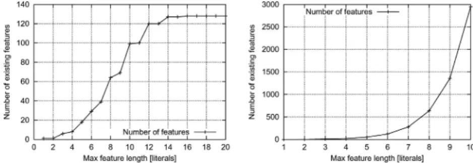
Fig. 2 Left: The number of features as a function of the maximum allowed feature length in the Trains domain where all declared predicates have at most one input argument. Right: The same dependence plotted for the same declaration extended by binary-input property predicatenotSame/2
individual (such asAin the examples above). There is at most 1+n·Mosuch variables and
ln+1has at most Miinput arguments. Therefore for each predicate chosen for ln+1, there is at
most (1+n·Mo)Mi choices of argument variables (output arguments acquire new distinct
variables), that is, the literal ln+1can be chosen in at most D·(1+n·Mo)Midifferent ways.
The search space thus contains at mostL
n=1D·(1+n·Mo)Mi ≤DL·(1+L·Mo)Mi·L
search nodes. Two exponential factors are present in this worst-case estimate: Mi — the
maximum input arity, and L — the maximum feature length. Out of the two, the former is of less interest to us, since it is typically set to a small constant in common application domains. For example, in the empirical evaluation (Krogel et al.,2003) conducted on six benchmark problems, Mihad the value 1 in four domains and 2 in two domains, in all cases
leading to a useful feature set (with respect to the predictive accuracy of the subsequently induced model of data built on the provided features). The latter parameter L is thus a crucial complexity factor of the algorithm—therefore it is used as the independent variable in most of the performance diagrams shown in this paper.
The above worst-case estimate ignores the moding and typing constraints. They may however significantly improve upon the estimate, which we illustrate empirically. The left panel of Figure2shows the actual number of features as a function of the maximum allowed definition length in the Trains domain where Mi =1 (no predicates with more than one
input argument are declared). Despite the estimated exponential-in-L growth, the function actually becomes constant at L=16. This is no longer the case when binary-input predicate
notSame/2is further declared (allowing to construct features such as (6) above). Here Mi =2 and the number of features grows exponentially with L.
RSD implements several pruning techniques to reduce the number of examined expres-sions, while preserving the exhaustiveness of the resulting feature set.
First, suppose that the currently explored expression f of length n contains o output variables not appearing also as input variables in f. Let the maximum number of input arguments of a predicate among all available background predicates be Miand L be the
maximum length of a feature. Then Rule 1. Once L−n≤ Mo
i, prune all descendants of f reached by adding a structural literal to it.
In other words, if the inequality holds, the algorithm will no longer consider to add structural predicates when refining f. By doing so it would introduce one or more new output variables; a simple calculation yields that there would not be enough literal positions left to make all output variables appear also as inputs.
The following two pruning rules exploit the constraint of feature undecomposability. The constraint is verified by maintaining a setϑeq(f) of equivalence classes of non-key variables
in each explored expression f. Two non-key variables X, Y fall in the same equivalence class iff they are connected, i.e., if they both appear as arguments in one literal of the expression, or there is a non-key variable Z such that X, Z are connected and Z, Y are connected. Expression f is a feature only if|ϑeq( f )| =1. Note that a feature may be reached by refining
a decomposable node. The following two pruning rules cut off the search subspaces which surely contain only decomposable nodes. Let us call a literal primary if all its input arguments hold the key variable.
Rule 2. If expression f is a non-empty conjunction, prune all its descendants reached by adding a primary property literal to it.
Rule 2 expresses the simple insight that adding a primary property literal to a feature definition will yield a decomposable feature.
Rule 3. Let expression f contain a primary literal lp.
1. If lpis a property literal, prune all descendants of f.
2. If lpis a structural literal and Mi=1, prune all descendants reached by adding a
primary structural literal to f.
The first item of pruning Rule 3 again avoids combining a primary property literal with any other literals. Now consider the case when the maximum input arity of available predicates is equal to 1 (the second item of Rule 3). This is natural in frequent cases when each structural predicate serves for addressing a part or a substructure of a single structure and property predicates do not relate two or more objects. For example, the earlier addressed Trains domain is a typical representant of the situation if the declared language excludes the binary predicatenotSame/2relating two cars. The second item of Rule 3 then captures the following idea. To reach a contradiction, let us assume that we can in fact arrive to an admissible feature definition that contains two primary structural literals l1and l2. Let oibe
some output variable of li(i=1, 2). Since the maximum input arity is 1, o1and o2cannot
be connected and the feature would be decomposable, that is, inadmissible.
Finally, it can be shown that Rules 2 and 3 cut off all decomposable nodes in the search tree when amax=1 and therefore we can skip decomposability checks as Rule 4 dictates.
Rule 4. If Mi=1, skip all decomposability checks.
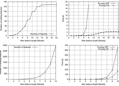
Figure3illustrates the impact of the described pruning techniques on the efficiency of the feature construction algorithm.
4.2. Employing constants and feature filtering
After constructing a constant-free feature set, RSD proceeds to ground selected variables in the features with constants extracted from the input data in the following manner. The user may declare a special property predicateinstantiate/1, just like other property predicates. An occurrence of this predicate in a feature with some variable V as its argument specifies that all occurrences of V in the feature should be eventually substituted with a constant. Theinstantiate/1literal may appear several times with different variables
Fig. 3 Empirical example of the impact of search space pruning during syntactic feature construction in the Trains domain. The diagrams on the left show the number of admissible features in the two settings described in Figure2(top: at most one input in any declared predicate, bottom: additional binary-input predicate) with the growing maximum feature length: we redisplay these dependencies for ease of comparison. To the right of each of them, we plot the time taken by the algorithm to complete the feature construction in the respective setting with pruning off and on. In the case of only-unary-properties (top), the number of features eventually stops growing, and so does the construction time taken by the pruning-enhanced algorithm as it correctly eliminates the growing search subspaces containing no correct feature. On the contrary, the non-pruning algorithm maintains its exponential time complexity. In the case of additional binary propertynotSame/2
(bottom), the time dependencies exhibit a similar shape, however, the efficiency gain of the pruning version is still essential
in a single feature. A number of different features are then generated, each corresponding to a possible grounding of the combination of the indicated variables. We consider only those groundings which make the feature true for at least a pre-specified number of individuals.
For example, after consulting the input data, the constant-free expression
hasCar(A,B),hasLoad(B,C),hasShape(C,D),instantiate(D) (7) is replaced by a set of features, in each of which theinstantiate/1literal is removed and theDvariable is substituted by a constant making the conjunction true for at least one individual, for example
hasCar(A,B),hasLoad(B,C),hasShape(C,rectangle) (8)
Feature filtering takes place within the described step of employing constants and con-forms to the following constraints. (a) No feature should have the same Boolean value for all the examples. (b) No two features should have the same Boolean values for all the examples (in this case, a single feature is chosen to represent the class of semantically equivalent
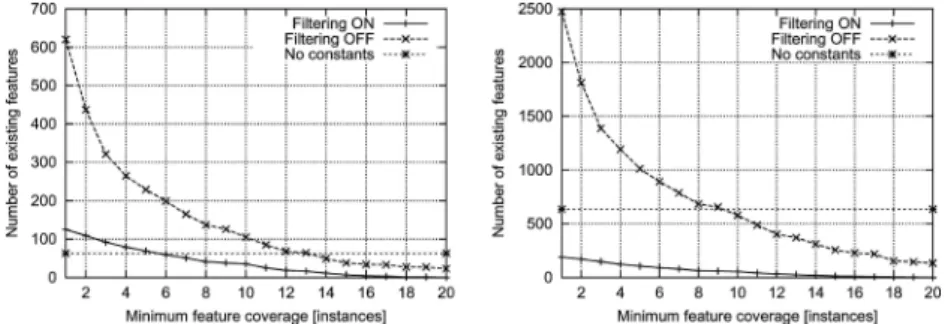
Fig. 4 The impact of feature filtering in the Trains domain in the two respective settings described in Figure 2(left: at most one input in any declared predicate, right: binary-input predicatenotSame/2added). “No constants”: the number of features generated before considering constants. “Filtering off”: the number of features after grounding them in several possible ways, each required to make the feature true for at least the number of instances on the X axis. “Filtering on”: the same dependency, but discarding a subset of features so that all resulting features have distinct and non-complete coverage
features). (c) A minimum number of examples for which a feature has to be true can be prescribed.
Figure4shows an empirical example of the impact of employing constants and feature filtering on the resulting number of features.
4.3. Generating a propositional representation
Having constructed the appropriate features, the user can obtain various forms of attribute-value representations of the relational input data. The system can produce either a generic ASCII file of an easily parameterizable format, or files serving as inputs to specific propo-sitional learners. Currently, the supported export formats are those of the RSD subgroup discovery component, the WEKA system (Witten et. al.,1999), the CN2 program (Clark & Niblett,1989) and the CN2-SD (Lavraˇc et al.,2004) propositional subgroup discovery algorithm which uses the same format as CN2.
5. RSD subgroup discovery
To identify a set of interesting subgroups, RSD applies the weighted covering algorithm (Section3.5, while individual rules are found by top-down heuristic beam-search, guided by a variant of the WRAcc search heuristic. The combination of the two principles implies the use of the following modified WRAcc heuristic:
WRAcc(H ←B)= n (B) N n(H B) n(B) − n(H ) N (9)
where N is the number of examples, Nis the sum of the weights of all examples, n(H) is the number of examples of class H, n(B) is the sum of the weights of all covered examples, and n(HB) is the sum of the weights of all correctly covered examples. Compared to the definition of the WRAcc heuristic used in CN2-SD (Lavraˇc et al.,2004), the definition of modified WRAcc in Eq. (9) has been improved: in contrast with the nN(H ) computation of
the prior probability in CN2-SD which changes with changed example weights, in RSD the prior probability computationn(H )N remains unchanged.
To add a rule to the generated rule set, the rule with the maximum modified WRAcc value is chosen from the set of searched rules not yet present in the rule set generated so far.
The constraints employed in the subgroup search include the language constraint of the maximal number of features considered in the subgroup description as well as several evaluation constraints. These include the minimal value of the significance formula (Clark & Niblett,1989) for each subgroup, as well as a minimal value threshold for the modified WRAcc function, which is exploited for sake of pruning.
Two pruning rules are used in the beam-search. According to the first, all refinements of a node will be pruned, if that node stands for a rule covering only instances of the target class, as such a rule cannot be improved by a refinement. Furthermore, if minimal value t is prescribed for WRAcc, we prune all refinements of rule H←B if the inequality
n(B) N 1−n(H ) N <t (10)
holds, as clearly no refinement thereof can yield a WRAcc value higher than the left-hand side of the inequality (weighted coverage will not grow when specializing, while weighted accuracy cannot exceed 1). Constraint (10) thus ensures that no rule is induced whose coveragenN(B) is so small that even if the rule had perfect accuracy p(H|B)=1, its coverage
vs. relative accuracy tradeoff computed by WRAcc would have been below t.
6. Experimental domains
In addition to three popular ILP data sets, the East-West trains (Trains), the King-Rook-King illegal chess endgame positions (KRK) and mutagenicity prediction (Mutagenesis), we have performed the experimental evaluation of RSD also on two other domains: a real-life telecommunications problem (Telecom) and the analysis of traffic accidents (Traffic). The Trains problem was used in earlier sections for explanatory purposes only.
6.1. Three ILP domains
We performed experiments on three popular ILP data sets: Trains, KRK and Mutagenesis.
Trains. We chose the 20 trains East-West challenge (Michie et al.,1994) as an illustrating example earlier in this paper. For these trains, information is given about their cars and the loads of these cars. The original classification task was to discover (low-complexity) models that classify trains as heading East or West. The subgroup discovery task addressed in this paper is to discover subgroups that are sufficiently large and biased towards one of the two classes: East and West.
KRK. In the chess endgame domain White King and Rook versus Black King, taken
from (Quinlan, 1990) (first described in Muggleton et al. (1989)), the target relation
illegal(A, B, C, D, E, F)states whether a position where the White King is at file and rank (A, B), the White Rook at (C, D) and the Black King at (E, F) is an illegal White-to-move position. For example,illegal (g,6,c,7,c,8)is a positive example, i.e., an illegal position. Two background predicates are available:lt/2
relation on such pairs. The data set consists of 1000 instances. The original predictive KRK task aimed at best distinguishing between illegal and legal chess endgame positions, whereas the subgroup discovery task aims at detecting groups of chessboard positions, distinguishable by means of the background relations, which contain an unusually large proportion of illegal/legal positions. In the KRK domain we do not expand features by instantiating variables to constants (as described in Section 4.2). This problem is thus ‘purely relational’.
Mutagenesis. The Mutagenesis problem defined in Srinivasan et al. (1996) is a variant of the original data named NS+S2 (also known as B4) that contains information about drugs: their chemical properties, the drugs’ atoms and the bonds between the atoms. The original Mutagenesis learning task was to predict whether a drug is mutagenic or not. The sepa-ration of data into ‘regression-friendly’ (188 instances) and ‘regression-unfriendly’ (42 instances) subsets as described by Srinivasan et al. (1996) is followed in our experiments. Our experiments concentrate on subgroup discovery from the ‘regression-friendly’ subset consisting of 188 instances.
6.2. The Telecom domain
We have applied RSD to a real-life problem in telecommunications. An extensive description of the nature of the data as well as tasks and problems that appear in this domain can be found in ˇZelezn´y et al. (2000,2002).
The data represent incoming calls (1995 items thereof) to an enterprise. Each call is answered by a human operator and in the usual case further transferred to an attendant distinguished by his/her line number. Further call transfers may also occur. Each sequence of such transfers is tracked by a computerized exchange and related data are stored in a log file. By a suitable transformation thereof, one can form a relationincoming/5, represented by ground facts of the formincoming(date, time, caller, operator, result). The argument result either takes a constant value or is a recursively defined function, so that result∈{talk, unavailable, transfer ([ln1, ln2, . . . , lnn], result)}, where ln1 ... lnn denote line
numbers to which transfer attempts were made (in the first n−1 cases unsuccessfully and in the n-th case with outcome result). For example, the following fact
incoming(date(10,18),time(13,37,29),[0,6,4,8,2,5,6,8,4,9],32, transfer([16,12],transfer([26],talk)))
describes a call from phone number 0648256849 at 13:37:29 on 10/18 received by the operator on line 32. The operator first tried to transfer the caller to line 16 without success, and then transferred him/her successfully to line 12. The person on line 12 further redirected the caller to line 26. After a talk with line 26, the call was terminated.
We divided all instances of incoming transferred calls into 25 classes determined by the line to which the operator tried to transfer the caller first. The arguments of the training instances thus consist of the first four arguments ofincoming/5, and the class label ln1.
The goal of subgroup discovery is to find subgroups biased to specific classes (destinations of first call transfer) which may be used to support operators’ decision making.
Let us now comment on two of the available background relations. The predicate pre-fix(Number,Prefix)is true whenever the second (output) argument is the prefix (of any length) of the first (input) argument. For instance, regarding the example given above,
prefix([0,6,4,8,2,5,6,8,4,9],[0,6,4])is true. This background predicate proved useful in previously published results, since it is able to bind callers from the same area, city, company, office etc.
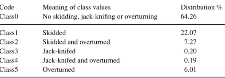
Table 2 The meaning and the distribution of class values in the UK Traffic challenge data set
Code Meaning of class values Distribution % Class0 No skidding, jack-knifing or overturning 64.26
Class1 Skidded 22.07
Class2 Skidded and overturned 7.27
Class3 Jack-knifed 0.20
Class4 Jack-knifed and overturned 0.19
Class5 Overturned 6.01
Another background predicate (prev\attempt/6) reflects the fact that a line desired by the caller may often be determined by looking at the caller’s recent attempts to reach a person, i.e., by inspecting past records (w.r.t. the time-label of the current example) in the
incoming/5relation. For example, the goal
prev attempt(date(10,18),time(13,37,29),[0,6,4,8,2,5,6,8,4,9], Line, When, Result)
will succeed with the result
Line = 10, When = today, Result = unavailable
provided the caller 0648256849 failed to reach line 10 on 10/18 before 13:37:29. Note that theprev attempt/6may yield multiple outputs for a given instantiation of the input arguments.
6.3. The UK Traffic Accidents Domain
The UK Traffic data set includes the records of all the accidents that happened on the roads of Great Britain between years 1979 and 1999 (Flach et al.,2003). It is a relational data set consisting of 3 related data tables: the ACCIDENT data, the VEHICLE data and the CASUALTY data. The ACCIDENT data consists of the records of all accidents that happened in the given time period; VEHICLE data includes data about all the vehicles involved in these accidents; CASUALTY data includes the data about all the casualties involved in the accidents. Consider the following example: ‘Two vehicles crashed in a traffic accident and three people were seriously injured in the crash’. In terms of the TRAFFIC data set this is recorded as one record in the ACCIDENT data table, two records in the VEHICLE data table and three records in the CASUALTY data table. Every data table is described by around 20 attributes and consists of more than 5 million records.
The UK Traffic challenge data set is formed of a subset of records of the above data set. The task of the challenge was to generate classification models to predict skidding and overturning. As the class attribute Skidding and Overturning appears in the VEHICLE data table, data tables ACCIDENT and VEHICLE were merged in order to make this a non-relational learning problem. Furthermore, a randomly sampled subset of 5940 records from this merged data table was selected for learning and another sample of 1585 records was selected for testing. The class attribute Skidding and Overturning has six possible values. The meaning of these values and the distribution of class values in the training and test sets are shown in Table2.
Table 3 Examples of generated features
KRK f6(A):-king1 rank(A,B),rook rank(A,C),adj(C,B). Meaning First king’s rank adjacent to rook’s rank.
Mutagenesis f12(A):-atm(A,B),atm chr(B,C),lteq c(C,0.142).
Meaning A compound contains an atom with charge less or equal to 0.142.
Mutagenesis f31(A):-benzene(A,B),benzene(A,C),connected(C,B).
Meaning Presence of two connected benzene rings in the compound.
Telecom f99(A):-ext number(A,B),prefix(B,[0,4,0,7]).
Meaning Caller’s number starts with 0407.
Telecom f115(A):-call date(A,B),call time(A,C),ext number(A,D),
prev attempt(B,C,D,[3,1],today,unavailable).
Meaning The caller of the current call has today tried to reach line 31, which was unavailable. While the original task of the challenge was to generate classification models to predict skidding and overturning, in our case, the task is to find subgroup descriptions representing interesting skidding and overturning patterns appearing in the Traffic challenge data set.
7. RSD propositionalization: Experimental evaluation
This section presents the experimental results. Experiments with feature construction and filtering are illustrated in three domains: KRK, Telecom and Mutagenesis. An experimental comparison of the RSD propositionalization procedure with the original first-order feature construction procedure (Flach & Lachiche, 1999; Lavraˇc & Flach 2001; Kramer et al.,
2001) as implemented in SINUS (Krogel et al.,2003) is performed in KRK, Trains and Mutagenesis.
7.1. Evaluation of feature construction and filtering
To generate features for KRK and Telecom, we use the background predicates described in the domains descriptions. For the KRK domain, we also allow to generate features in the form of a negation of a complete literal conjunction.
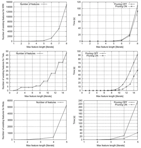
Figure5reflects the quantitative characteristics of RSD syntactic feature construction and the effect of pruning in the three domains, from the viewpoint we took in the Trains domain in Figure3. The efficiency gain by the earlier described search space pruning techniques is not very significant in the KRK domain, but becomes essential with growing feature length in Telecom and Mutagenesis.
Table 3shows examples of features generated in the KRK, Mutagenesis and Telecom domains.
7.2. Experimental comparison with SINUS
This section compares the RSD propositionalization procedure with the first-order feature construction procedure (Flach & Lachiche, 1999; Lavraˇc & Flach,2001; Kramer et al.,
2001) implemented in SINUS (Krogel et al.,2003).
SINUS was first implemented as an extension to the original LINUS transformational ILP learner (Lavraˇc & Dˇzeroski,1994). LINUS performs the transformation to a propositional representation by considering only possible applications of background predicates on the
Fig. 5 Number of features (left) and impact of pruning in RSD syntactic feature construction on efficiency (right) in KRK, Telecom and Mutagenesis, shown in dependence to the maximum allowed length of a feature. This viewpoint corresponds to Figure3for the example domain of Trains
arguments of the target relation, taking into account the types of arguments. The clauses it learns are constrained. The development of DINUS (Lavraˇc & Dˇzeroski,1994) relaxed this bias so that non-constrained clauses can be constructed provided that the clauses involved are determinate. SINUS was later extended to perform propositionalization by extended first-order feature construction described in Flach and Lachiche (1999), Lavraˇc and Flach (2001) and Kramer et al., (2001).10
The RSD propositionalization has the following advantages compared to SINUS. It pro-vides a declaration language similar to Progol for fine-tuning syntactic constraints on features, it verifies the undecomposability of features and offers improvements (pruning techniques in the feature search, coverage-based feature filtering). These improvements lead to improved efficiency of propositionalization as shown in the experiments of this section.
10Detailed information about SINUS is available from the SINUS website at
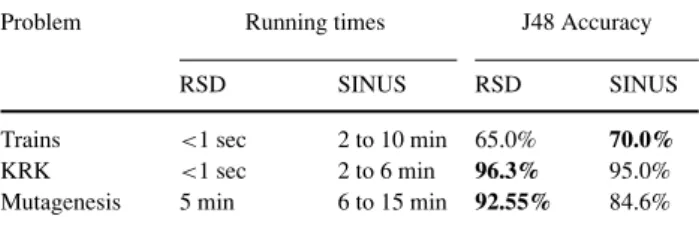
Table 4 Indicators of running times (different platforms, cf. text) and systems providing the feature set for the best-accuracy result in each domain
Problem Running times J48 Accuracy
RSD SINUS RSD SINUS
Trains <1 sec 2 to 10 min 65.0% 70.0%
KRK <1 sec 2 to 6 min 96.3% 95.0%
Mutagenesis 5 min 6 to 15 min 92.55% 84.6%
As RSD and SINUS are implemented in different languages (interpreters) and operate on different hardware platforms, exact comparison of runtime efficiency is not possible. As in Krogel et al. (2003), for each domain and system we report the approximate running times, averaged over multiple feature construction runs, varying in the language constraints and producing feature sets of different sizes. RSD ran under the Yap Prolog on a Celeron 800 MHz computer with 256 MB of RAM. SINUS ran under SICStus Prolog11on a Sun
Ultra 10 computer. Table4shows running times of the propositionalization systems on the learning tasks (with best results indicated in bold). The table also provides 10-fold stratified cross-validation accuracy results of applying the J48 propositional learner (a reimplemen-tation of C4.5 (Quinlan,1993) available in WEKA (Witten & Frank,1999)), supplied with propositionalized data based on feature sets of varying size obtained from the two proposi-tionalization systems. To test the performance of the two systems, producing the accuracy results in Table4, RSD and SINUS were used to construct features by different parameter settings; the results of 10-fold stratified cross-validation for the best setting are shown.
Different performance of RSD and SINUS are due to their different ways of constrain-ing the language bias. RSD wins in the KRK domain and Mutagenesis. While the gap on KRK seems little significant, the result obtained on Mutagenesis with RSD’s 25 features12is
competitive to the best results reported in the ILP literature. Whether the apparent efficiency superiority of RSD w.r.t SINUS is due to the RSD’s pruning mechanisms, or the implemen-tation in the faster Yap Prolog, or a combined effect thereof has to be investigated in more depth in future work.
8. RSD subgroup discovery: Experimental evaluation
For the experimental domains Trains, KRK, Mutagenicity and Telecom, parts of the experi-mental settings overlap, and parts are unique for each of the domains. The common parts of the experimental procedures are outlined below. A separate evaluation procedure is used in the Traffic challenge domain as the goal is to compare RSD with SubgroupMiner in terms of the AUC performance.
The RSD algorithm was run as follows.
11It should be noted that SICStus Prolog is generally considered to be several times slower than Yap prolog. 12The longest have 5 literals in their bodies. Prior to irrelevant-feature filtering conducted by RSD, the feature
– For each dataset we first ran the RSD propositionalization procedure. We generated a set
of features and—when applicable—expanded the set with features containing variable instantiations. We then used the feature sets to produce a propositional representation of each of the data sets. The results of this evaluation were presented in Section7.1.
– We then ran the RSD subgroup discovery procedure to construct interesting subgroups
from the propositional data. In this procedure we have subsequently exchanged the RSD’s WRAcc heuristic with the standard accuracy (Acc) heuristic, and the RSD’s weighted cov-ering algorithm with the standard covcov-ering algorithm, thereby testing four configurations of the method. Results of each are compared in terms of subgroup interestingness criteria. See the list of subgroup evaluation criteria in Section2and the results of the evaluation in Section8.1.
The generation of stratified cross-validation splits and subsequent assessment of resulting rules is done automatically by the RSD system. The experiments are repeatable, as the RSD package available athttp://labe.felk.cvut.cz/∼zelezny/rsdcontains scripts needed to conduct the experimental procedures automatically to achieve the results presented below. 8.1. Subgroup discovery evaluation results
In the experiments we used different variants of the RSD rule learning algorithm by altering the covering strategy and the heuristic function used to construct sets of subgroup-describing rules.
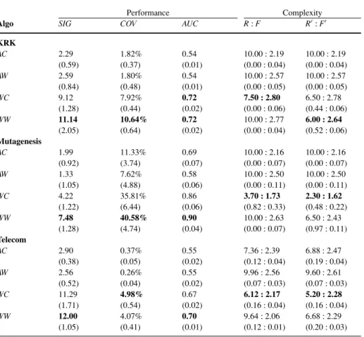
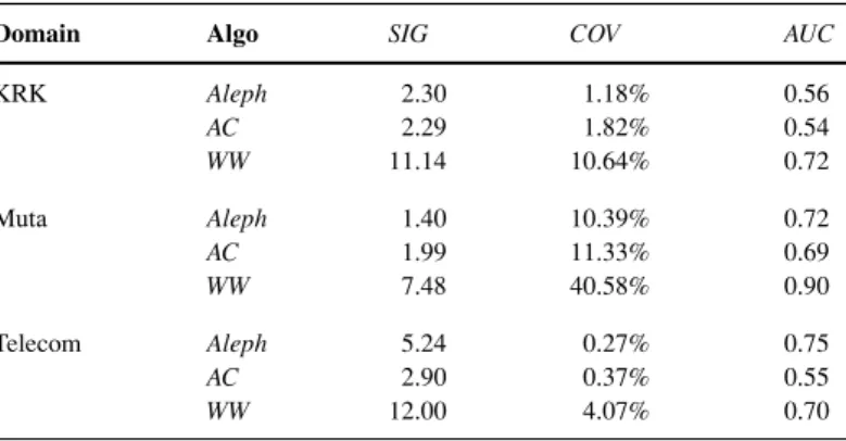
Achieved results and characteristics of discovered rules are shown in Table5, where Algo refers to the combination of the search heuristic (A – accuracy, W – weighted relative accuracy) and the covering algorithm (C – covering, W – weighted covering using additive weights). Results are evaluated in terms of the following interestingness criteria: SIG – significance, COV - coverage, AUC – area under the ROC curve, R : F – average number of rules per class : average number of features per rule, R: F– the same as above, but considering only the rules on the ROC convex hull. The reported results are averages obtained in 10-fold stratified cross-validation, along with the corresponding standard deviations.
Rule generation for a given class was terminated if the search space was completely ex-plored or the maximal number of subgroup rules was generated (10 subgroup rules generated for KRK and Telecom, and 5 for Mutagenesis).
The most important observation about the results in Table 5 is that, in terms of all the quality criteria, the RSD’s WRAcc heuristic very significantly improves the performance compared to the standard accuracy heuristic. Overall, the combination of the WRAcc heuristic with the strategy of example weighting used in the weighted covering algorithm yields the best results. This agrees with the findings in (Lavraˇc et al.,2004), where a more extensive empirical evaluation was conducted on a collection of (non-relational) subgroup discovery problems, comparing the CN2 algorithm with CN2 incorporating a variant of the WRAcc heuristic, and further with the CN2-SD system (which incorporates a variant of the WRAcc heuristic and the weighted covering algorithm). These three algorithms roughly correspond to the methods we denote above (in Table5) as AC, WC, and WW, respectively. The combination of the accuracy heuristic with example weighting AW performs worse in the domains considered. 8.2. Expert analysis of induced subgroups
We now present selected subgroups, discovered by RSD in the KRK and Telecom domains, to illustrate the character of induced rules. We also present their pie-chart visualization.
Table 5 Results of ten-fold cross-validation obtained by the RSD algorithm in the KRK, Mutagenesis and Telecom domains (with standard deviations in parentheses)
Performance Complexity
Algo SIG COV AUC R : F R: F
KRK AC 2.29 1.82% 0.54 10.00 : 2.19 10.00 : 2.19 (0.59) (0.37) (0.01) (0.00 : 0.04) (0.00 : 0.04) AW 2.59 1.80% 0.54 10.00 : 2.57 10.00 : 2.57 (0.84) (0.48) (0.01) (0.00 : 0.05) (0.00 : 0.05) WC 9.12 7.92% 0.72 7.50 : 2.80 6.50 : 2.78 (1.28) (0.44) (0.02) (0.00 : 0.06) (0.44 : 0.06) WW 11.14 10.64% 0.72 10.00 : 2.77 6.00 : 2.64 (2.05) (0.64) (0.02) (0.00 : 0.04) (0.52 : 0.06) Mutagenesis AC 1.99 11.33% 0.69 10.00 : 2.16 10.00 : 2.16 (0.92) (3.74) (0.07) (0.00 : 0.07) (0.00 : 0.07) AW 1.33 7.62% 0.58 10.00 : 2.50 10.00 : 2.50 (1.05) (4.88) (0.06) (0.00 : 0.11) (0.00 : 0.11) WC 4.22 35.81% 0.86 3.70 : 1.73 2.30 : 1.62 (1.22) (6.44) (0.06) (0.82 : 0.33) (0.48 : 0.22) WW 7.48 40.58% 0.90 10.00 : 2.63 6.50 : 2.43 (1.28) (4.74) (0.04) (0.00 : 0.07) (0.97 : 0.11) Telecom AC 2.90 0.37% 0.55 7.36 : 2.39 6.88 : 2.47 (0.38) (0.05) (0.02) (0.12 : 0.04) (0.19 : 0.04) AW 2.56 0.26% 0.55 9.96 : 2.56 9.60 : 2.61 (0.52) (0.04) (0.02) (0.07 : 0.03) (0.07 : 0.03) WC 11.29 4.98% 0.67 6.12 : 2.17 5.20 : 2.28 (1.71) (0.54) (0.02) (0.16 : 0.04) (0.16 : 0.04) WW 12.00 4.07% 0.70 9.64 : 2.06 6.68 : 2.29 (1.05) (0.41) (0.01) (0.12 : 0.01) (0.20 : 0.03)
Table 6 A subgroup description induced in the KRK domain in the form H←B [TP,FP], its interpretation and definitions of features appearing as literals in the conjunctive antecedent of a rule describing the subgroup
Subgroup KRK1for target class:legal
legal(A) ← f139(A)∧f145(A)∧f133(A)[279,4]
f139(A):-not(rook rank(A,B),king2 rank(A,C),adj(C,C),adj(C,B)).
f145(A):-not(rook file(A,B),king2 file(A,C),adj(C,C),adj(C,B)).
f133(A):-not(king1 file(A,B),king2 file(A,C),adj(C,C),adj(C,B)). Configurations where rook’s rank is not adjacent to second king’s rank and rook’s file not adjacent to
second king’s file and first king’s file not adjacent to second king’s file (note thatadj(C,C)is always true, i.e. redundant).
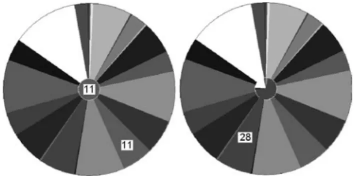
Table6presents a subgroup, induced in the KRK domain, and lists the Prolog notation of the features used as antecedent literals in the rule that describes the subgroup. The graphical presentation of the class distribution and coverage of the subgroup, illustrated at the right-hand side of Figure6, is complemented in Table6by a verbal description of the subgroup, together with the number of true positive (TP) and false positive (FP) examples covered.
Fig. 6 Left: SubgroupTrains1described in Table1of Section2. Right: SubgroupKRK1described in Table6of this section
Fig. 7 Left: Prior distribution of classes in the Telecom domain. Right: Subgroup Tele1 described in Table 7of this section
Fig. 8 Left: Subgroup Tele2, Right: SubgroupTele4, both described inTable 7of this section Figures6–8show pie-chart representations of the distributional characteristics of induced subgroups. In the outer pie, each area representing a class is proportional to the frequency of that class in the data set. Similarly, areas in the inner pie are proportional to the frequencies of corresponding classes in the subgroup. The ratio of the overall area of the inner pie to the area of the whole pie is the ratio between the number of instances included in the subgroup in and the number of all the instances in the respective data set.
In the Telecom domain, although exactly one class is the target, it often follows from the illustrated posterior distribution that the rule consequent can naturally be interpreted as a
Table 7 Telecom subgroup descriptions in the form H←B [TP,FP], definitions of used features, and subgroup interpretation including expert’s comments
Tele1: line21(A) ← f40(A) [56,268]
f40(A):-call date(A,B), dow(B,fri). Calls received on Fridays.
Expert’s evaluation: Not a novel information.
Tele2: line11(A)← f132(A) [32,0]
f132(A):-ext number(A,B), prefix(B,[8,5,1,3,1,1,1,1]). Calls received from number 85131111.
Expert’s explanation: The caller is the secretary’s husband. She does not have a direct-access line, thus this call is transferred by an operator.
Expert’s evaluation: Novel information.
Remark. Although the last literal formally identifies a prefix of the calling number, it is in fact the complete number of the caller.
Tele3: line21(A) ← f54(A) [81,254]
f54(A):-ext number(A,B), prefix(B,[0,4]). Calls received from a number that starts with 04.
Expert’s explanation: Prefix 04 is too general (code covers a large area) to find an explanation. Expert’s evaluation: Novel information. Uncertain.
Tele4: line28(A) ← f7(A) [22,11]
f7(A):-call date(A,B), call time(A,C),
ext number(A,D), prev attempt(B,C,D,[2,1],last hour,unavailable).
Calls received from a caller who has in the last hour attempted to directly (not through an operator) reach line 28, which was unavailable.
Expert’s explanation: It is plausible that people try line 28 as the second attempt when line 21 is unavailable. Subgroup probably mostly covers people with technical difficulties with a product sold by person on line 21.
Expert’s evaluation: Novel information.
disjunction of classes. This applies in cases when a subgroup contains instances of only a few classes, as opposed to the prior distribution of 25 classes.13
We now present the descriptions of some of the discovered subgroups in Telecom, with comments from the domain expert on the descriptions in Table 7 and the distributional characteristics of the subgroups in terms of the number of true positives (TP) and false positives (FP).
Expert analysis of the induced rules shows that some of them identify novel and interesting information. Especially revealing are the comments related to the changes of class frequency associated with the rules, as illustrated in the pie-charts. In the overall distribution, calls to line 21 are the most common. The expert commented that this reflects his expectations, as the person at line 21 is a marketer, and people interested in products call this line most frequently. In subgroupTele1, there is (a) an increase in line 21 frequency: clients not receiving an ordered package often wait until Friday and then complain with line 21; and (b) a decrease in line 13 frequency: the person at line 13 mostly collaborates with dealers who have less business on Fridays. For subgroupTele4there is (a) an increase in line 28 frequency: repeated attempts to reach line 28, and (b) an increase in line 21
13Note that only 15 classes are visible in the outer pies in the Telecom domain, as instances of the remaining