University of Massachusetts Amherst
ScholarWorks@UMass Amherst
Open Access Dissertations
9-2010
Optimization-based Approximate Dynamic
Programming
Marek Petrik
University of Massachusetts Amherst, [email protected]
Follow this and additional works at:
https://scholarworks.umass.edu/open_access_dissertations
Part of the
Computer Sciences Commons
This Open Access Dissertation is brought to you for free and open access by ScholarWorks@UMass Amherst. It has been accepted for inclusion in Open Access Dissertations by an authorized administrator of ScholarWorks@UMass Amherst. For more information, please contact
Recommended Citation
Petrik, Marek, "Optimization-based Approximate Dynamic Programming" (2010).Open Access Dissertations. 308. https://scholarworks.umass.edu/open_access_dissertations/308
OPTIMIZATION-BASED APPROXIMATE DYNAMIC PROGRAMMING
A Dissertation Presented by
MAREK PETRIK
Submitted to the Graduate School of the
University of Massachusetts Amherst in partial fulfillment of the requirements for the degree of
DOCTOR OF PHILOSOPHY September 2010
c
Copyright by Marek Petrik 2010 All Rights Reserved
OPTIMIZATION-BASED APPROXIMATE DYNAMIC PROGRAMMING
A Dissertation Presented by
MAREK PETRIK
Approved as to style and content by:
Shlomo Zilberstein, Chair
Andrew Barto, Member
Sridhar Mahadevan, Member
Ana Muriel, Member
Ronald Parr, Member
Andrew Barto, Department Chair Department of Computer Science
ACKNOWLEDGMENTS
I want to thank the people who made my stay at UMass not only productive, but also very enjoyable. I am grateful to my advisor, Shlomo Zilberstein, for guiding and supporting me throughout the completion of this work. Shlomo’s thoughtful advice and probing ques-tions greatly influenced both my thinking and research. His advice was essential not only in forming and refining many of the ideas described in this work, but also in assuring that I become a productive member of the research community. I hope that, one day, I will be able to become an advisor who is just as helpful and dedicated as he is.
The members of my dissertation committee were indispensable in forming and steering the topic of this dissertation. The class I took with Andrew Barto motivated me to probe the foundations of reinforcement learning, which became one of the foundations of this the-sis. Sridhar Mahadevan’s exciting work on representation discovery led me to deepen my understanding and appreciate better approximate dynamic programming. I really appre-ciate the detailed comments and encouragement that Ron Parr provided on my research and thesis drafts. Ana Muriel helped me to better understand the connections between my research and applications in operations research. Coauthoring papers with Jeff Johns, Bruno Scherrer, and Gavin Taylor was a very stimulating and learning experience. My re-search was also influenced by interactions with many other rere-searches. The conversations with Raghav Aras, Warren Powell, Scott Sanner, and Csaba Szepesvari were especially il-luminating. This work was also supported by generous funding from the Air Force Office of Scientific Research.
Conversations with my lab mate Hala Mostafa made the long hours in the lab much more enjoyable. While our conversations often did not involve research, those that did, moti-vated me to think deeper about the foundations of my work. I also found sharing ideas with my fellow grad students Martin Allen, Chris Amato, Alan Carlin, Phil Kirlin, Akshat
Kumar, Sven Seuken, Siddharth Srivastava, and Feng Wu helpful in understanding the broader research topics. My free time at UMass kept me sane thanks to many great friends that I found here.
Finally and most importantly, I want thank my family. They were supportive and helpful throughout the long years of my education. My mom’s loving kindness and my dad’s intense fascination with the world were especially important in forming my interests and work habits. My wife Jana has been an incredible source of support and motivation in both research and private life; her companionship made it all worthwhile. It was a great journey.
ABSTRACT
OPTIMIZATION-BASED APPROXIMATE DYNAMIC PROGRAMMING
SEPTEMBER 2010
MAREK PETRIK
Mgr., UNIVERZITA KOMENSKEHO, BRATISLAVA, SLOVAKIA M.Sc., UNIVERSITY OF MASSACHUSETTS AMHERST Ph.D., UNIVERSITY OF MASSACHUSETTS AMHERST
Directed by: Professor Shlomo Zilberstein
Reinforcement learning algorithms hold promise in many complex domains, such as re-source management and planning under uncertainty. Most reinforcement learning algo-rithms are iterative — they successively approximate the solution based on a set of samples and features. Although these iterative algorithms can achieve impressive results in some domains, they are not sufficiently reliable for wide applicability; they often require ex-tensive parameter tweaking to work well and provide only weak guarantees of solution quality.
Some of the most interesting reinforcement learning algorithms are based on approximate dynamic programming (ADP). ADP, also known as value function approximation, approx-imates the value of being in each state. This thesis presents new reliable algorithms for ADP that use optimization instead of iterative improvement. Because theseoptimization– basedalgorithms explicitly seek solutions with favorable properties, they are easy to an-alyze, offer much stronger guarantees than iterative algorithms, and have few or no pa-rameters to tweak. In particular, we improve on approximate linear programming — an
existing method — and derive approximate bilinear programming — a new robust ap-proximate method.
The strong guarantees of optimization–based algorithms not only increase confidence in the solution quality, but also make it easier to combine the algorithms with other ADP com-ponents. The other components of ADP are samples and features used to approximate the value function. Relying on the simplified analysis of optimization–based methods, we derive new bounds on the error due to missing samples. These bounds are simpler, tighter, and more practical than the existing bounds for iterative algorithms and can be used to evaluate solution quality in practical settings. Finally, we propose homotopy meth-ods that use the sampling bounds to automatically select good approximation features for optimization–based algorithms. Automatic feature selection significantly increases the flexibility and applicability of the proposed ADP methods.
The methods presented in this thesis can potentially be used in many practical applications in artificial intelligence, operations research, and engineering. Our experimental results show that optimization–based methods may perform well on resource-management prob-lems and standard benchmark probprob-lems and therefore represent an attractive alternative to traditional iterative methods.
CONTENTS
Page
ACKNOWLEDGMENTS . . . v
ABSTRACT. . . .vii
LIST OF FIGURES . . . xiv
CHAPTER 1. INTRODUCTION . . . 1
1.1 Planning Models . . . 3
1.2 Challenges and Contributions . . . 5
1.3 Outline . . . 8
PART I: FORMULATIONS 2. FRAMEWORK: APPROXIMATE DYNAMIC PROGRAMMING . . . 12
2.1 Framework and Notation. . . 12
2.2 Model: Markov Decision Process. . . 13
2.3 Value Functions and Policies. . . 16
2.4 Approximately Solving Markov Decision Processes. . . 23
2.5 Approximation Error: Online and Offline. . . 31
2.6 Contributions . . . 34
3. ITERATIVE VALUE FUNCTION APPROXIMATION. . . 35
3.1 Basic Algorithms . . . 35
3.3 Monotonous Approximation: Achieving Convergence. . . 43
3.4 Contributions . . . 44
4. APPROXIMATE LINEAR PROGRAMMING: TRACTABLE BUT LOOSE APPROXIMATION . . . 45
4.1 Formulation. . . 45
4.2 Sample-based Formulation . . . 49
4.3 Offline Error Bounds. . . 52
4.4 Practical Performance and Lower Bounds. . . 54
4.5 Expanding Constraints. . . 57
4.6 Relaxing Constraints. . . 62
4.7 Empirical Evaluation. . . 67
4.8 Discussion . . . 69
4.9 Contributions . . . 70
5. APPROXIMATE BILINEAR PROGRAMMING: TIGHT APPROXIMATION . . . 71
5.1 Bilinear Program Formulations . . . 71
5.2 Sampling Guarantees . . . 81
5.3 Solving Bilinear Programs. . . 83
5.4 Discussion and Related ADP Methods. . . 85
5.5 Empirical Evaluation. . . 90
5.6 Contributions . . . 93
PART II: ALGORITHMS 6. HOMOTOPY CONTINUATION METHOD FOR APPROXIMATE LINEAR PROGRAMS . . . .95
6.1 Homotopy Algorithm. . . 96
6.2 Penalty-based Homotopy Algorithm . . . 101
6.3 Efficient Implementation . . . 106
6.4 Empirical Evaluation. . . 108
6.5 Discussion and Related Work. . . 109
6.6 Contributions . . . 111
7.1 Solution Approaches. . . 113
7.2 General Mixed Integer Linear Program Formulation. . . 114
7.3 ABP-Specific Mixed Integer Linear Program Formulation . . . 117
7.4 Homotopy Methods . . . 119
7.5 Contributions . . . 122
8. SOLVING SMALL-DIMENSIONAL BILINEAR PROGRAMS . . . 123
8.1 Bilinear Program Formulations . . . 124
8.2 Dimensionality Reduction. . . 126
8.3 Successive Approximation Algorithm . . . 131
8.4 Online Error Bound. . . 136
8.5 Advanced Pivot Point Selection. . . 140
8.6 Offline Bound . . . 146
8.7 Contributions . . . 147
PART III: SAMPLING, FEATURE SELECTION, AND SEARCH 9. SAMPLING BOUNDS . . . 150
9.1 Sampling In Value Function Approximation . . . 151
9.2 State Selection Error Bounds. . . 154
9.3 Uniform Sampling Behavior. . . 161
9.4 Transition Estimation Error . . . 162
9.5 Implementation of the State Selection Bounds. . . 167
9.6 Discussion and Related Work. . . 170
9.7 Empirical Evaluation. . . 173
9.8 Contributions . . . 177
10. FEATURE SELECTION. . . 178
10.1 Feature Considerations. . . 179
10.2 Piecewise Linear Features . . . 180
10.3 Selecting Features. . . 183
10.4 Related Work. . . 187
10.5 Empirical Evaluation. . . 191
11. HEURISTIC SEARCH. . . 194
11.1 Introduction. . . 195
11.2 Search Framework. . . 200
11.3 Learning Heuristic Functions . . . 204
11.4 Feature Combination as a Linear Program . . . 218
11.5 Approximation Bounds . . . 225 11.6 Empirical Evaluation. . . 231 11.7 Contributions . . . 234 12. CONCLUSION . . . 235 PART: APPENDICES APPENDICES A. NOTATION . . . 239 B. PROBLEM DESCRIPTIONS. . . . 242 C. PROOFS. . . 250 BIBLIOGRAPHY. . . 335
LIST OF FIGURES
Figure Page
1 Chapter Dependence. . . xviii
1.1 Blood Inventory Management . . . 1
1.2 Reservoir Management. . . 2
1.3 Optimization Framework . . . 7
2.1 Transitive-feasible value functions in an MDP with a linear state-space. . . 19
2.2 Approximate Dynamic Programming Framework. . . 24
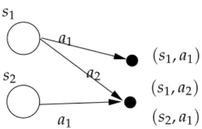
2.3 Example of equivalence of pairs of state-action values.. . . 27
2.4 Sample types. . . 28
2.5 Online and offline errors in value function approximation. . . 32
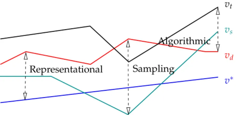
2.6 Value functions and the components of the approximation error. . . 33
4.1 Sampled constraint matrixAof the approximate linear program. . . 52
4.2 An example chain problem with deterministic transitions and reward denoted above the transitions. . . 56
4.3 Approximation errors in approximate linear programming. . . 57
4.4 Illustration of the value function in the inventory management problem. . . 57
4.5 An example of 2-step expanded constraints (dashed) in a deterministic problem. The numbers next to the arcs represent rewards. . . 58
4.6 Benchmark results for the chain problem.. . . 67
4.7 Bound onL1approximation error with regard to the number of expanded constraints on the mountain car problem.. . . 69
5.1 L∞ Bellman residual for the chain problem. . . 91
5.2 Expected policy loss for the chain problem. . . 91
5.3 Robust policy loss for the chain problem. . . 92
6.1 Comparison of performance of homotopy method versus Mosek as a function ofψin the mountain car domain. The Mosek solutions are recomputed in increments for values ofψ. . . 109
6.2 Comparison of performance of homotopy method versus Mosek as a function ofψin the mountain car domain. The Mosek solutions are computed for the final value ofψonly. . . 110
7.1 An illustration ofθBand the property satisfied byθB(ψ¯).. . . 122
8.1 Approximation of the feasible setYaccording to Assumption 8.3. . . 128
8.2 Refinement of a polyhedron in two dimensions with a pivoty0. . . 136
8.3 The reduced setYhthat needs to be considered for pivot point selection.. . . 140
8.4 ApproximatingYhusing the cutting plane elimination method.. . . 143
9.1 Value of a feature as a function of the embedded value of a state. . . 157
9.2 Comparison between the best-possible local modeling (LM) and a naive Gaussian process regression (GP) estimation ofep/e∗p. The results are an average over 50 random (non-uniform) sample selections. The table shows the mean and the standard deviation (SD). . . 175
9.3 Comparison between the local modeling assumption and the Gaussian process regression for the Bellman residual for featureφ8and actiona5 (functionρ1) and the reward for actiona1(functionρ2). Only a subset of k(S)is shown to illustrate the detail. The shaded regions represent possible regions of uncertainties.. . . 175
9.4 Comparison between the local modeling assumption and the Gaussian process regression for the Bellman residual for featureφ8and actiona5
(functionρ1) and the reward for actiona1(functionρ). The shaded
regions represent possible regions of uncertainties. . . 175 9.5 Uncertainty of the samples in reservoir management for the independent
samples and common random numbers.. . . 176 9.6 Transition estimation error as a function of the number of sampled states.
The results are an average over 100 permutations of the state order.. . . 177 10.1 Examples of two piecewise linear value functions using the same set of 3
features. In blood inventory management,xandymay represent the
amounts of blood in the inventory for each blood type. . . 181 10.2 Sketch of error bounds as a function of the regularization coefficient. Here,
v1is the value function of the full ALP,v3is the value function of the
estimated ALP, andv∗is the optimal value function.. . . 184 10.3 Comparison of the objective value of regularized ALP with the true
error. . . 192 10.4 Comparison of the performance regularized ALP with two values ofψand
the one chosen adaptively (Corollary 10.5). . . 192 10.5 Average of 45 runs of ALP and regularized ALP as a function of the
number of features. Coefficientψwas selected using Corollary 10.5. . . 192 11.1 Framework for learning heuristic functions. The numbers in parentheses
are used to reference the individual components.. . . 197 11.2 Examples of inductive methods based on the inputs they use. . . 208 11.3 Bellman residual of three heuristic functions for a simple chain
problem. . . 215 11.4 Three value functions for a simple chain problem . . . 215 11.5 Formulations ensuring admissibility. . . 220 11.6 Lower bound formulations, where the dotted lines represent paths of
11.7 An approximation with loose bounds.. . . 228
11.8 An example of the Lyapunov hierarchy. The dotted line represents a constraint that needs to be removed and replaced by the dashed ones.. . . 229
11.9 Weights calculated for individual features using the first basis choice. Columnxicorresponds to the weight assigned to feature associated with tilei, where 0 is the empty tile. The top 2 rows are based on data from blind search, and the bottom 2 on data from search based on the heuristic from the previous row. . . 233
11.10The discovered heuristic functions as a function ofαin the third basis choice, wherexi are the weights on the corresponding features in the order they are defined. . . 233
B.1 A sketch of the blood inventory management . . . 244
B.2 Rewards for satisfying blood demand.. . . 245
B.3 The blood flow in blood inventory management.. . . 246
C.1 MDP constructed from the corresponding SAT formula. . . 300
C.2 FunctionθBfor the counterexample.. . . 311
C.3 A plot of a non-convex best-response functiongfor a bilinear program, which is not in a semi-compact form.. . . 320
Sampling Bounds (9)
Small-Dim ABP (8) Introduction (1) Heuristic Search (11)
Framework (2) Iterative Methods (3)
ALP (4) ABP (5)
Solving ABP (7)
Features (10) Homotopy ALP (6)
CHAPTER 1
INTRODUCTION
Planning is the process of creating a sequence of actions that achieve some desired goals. Typical planning problems are characterized by a structured state space, a set of possible actions, a description of the effects of each action, and an objective function. This thesis treats planning as an optimization problem, seeking to find plans that minimize the cost of reaching the goals or some other performance measure.
Automatic planning in large domains is one of the hallmarks of intelligence and is, as a result, a core research area of artificial intelligence. Although the development of truly general artificial intelligence is decades — perhaps centuries — away, problems in many practical domains can benefit tremendously from automatic planning. Being able to adap-tively plan in an uncertain environment can significantly reduce costs, improve efficiency, and relieve human operators from many mundane tasks. The two planning applications below illustrate the utility of automated planning and the challenges involved.
AB A 0 Sto ch as ti c Su pp ly Blood Bank Hospital 2 Hospital 1 A B Sto ch as ti c D ema nd
Reservoir Irrigation
Water Inflow
Electricity Price
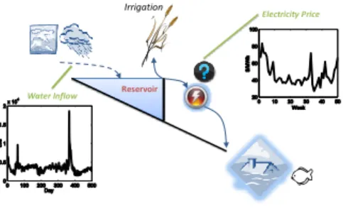
Figure 1.2.Reservoir Management
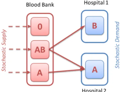
Blood inventory management A blood bank aggregates a supply of blood and keeps an
inventory to satisfy hospital demands. The hospital demands are stochastic and hard to predict precisely. In addition, blood ages when it is stored and cannot be kept longer than a few weeks. The decision maker must decide on blood-type substitutions that minimize the chance of future shortage. Because there is no precise model of blood demand, the solution must be based on historical data. Even with the available historical data, calculating the optimal blood-type substitution is a large stochastic problem. Figure 1.1 illustrates the blood inventory management problem andSection B.2describes the formulation in more detail.
Water reservoir management An operator needs to decide how much and when to
dis-charge water from a river dam in order to maximize energy production, while satisfying irrigation and flood control requirements. The challenges in this domain are in some sense complementary to blood inventory management with fewer decision options but greater uncertainty in weather and energy prices.Figure 1.2illustrates the reservoir management problem andSection B.3describes the formulation in more detail.
Many practical planning problems are solved usingdomain-specificmethods. This entails building specialized models, analyzing their properties, and developing specialized algo-rithms. For example, blood inventory and reservoir management could be solved using the standard theory of inventory management (Axsater, 2006). The drawback of special-ized methods is their limited applicability. Applying them requires significant human
ef-fort and specialized domain knowledge. In addition, the domain can often change during the lifetime of the planning system.
Domain-specific methods may also be inapplicable if the domain does not clearly fit into an existing category. For example, because of the compatibility among blood types, blood inventory management does not fit well the standard inventory control framework. In reservoir management, the domain-specific methods also do not treat uncertainty satisfac-torily, neither do they work easily with historical data (Forsund, 2009).
This thesis focuses on general planning methods — which are easy to apply to a variety of settings — as an alternative to domain–specific ones. Having general methods that can reliably solve a large variety of problems in many domains would enable widespread application of planning techniques. The pinnacle of automatic planning, therefore, is to develop algorithms that work reliably in many settings.
1.1 Planning Models
The purpose of planning models is to capture prior domain knowledge, which is crucial in developing appropriate algorithms. The models need to capture the simplifying properties of given domains and enable more general application of the algorithms.
A planning model must balance domain specificity with generality. Very domain-specific models, such as the traveling salesman problem, may be often easy to study but have limited applicability. In comparison, very general models, such as mixed integer linear programs, are harder to study and their solution methods are often inefficient.
Aside from generality, the suitability of a planning model depends on the specific prop-erties of the planning domain. For example, many planning problems in engineering can be modeled using partial differential equations (Langtangen, 2003). Such models can cap-ture faithfully continuous physical processes, such as rotating a satellite in the orbit. These models also lead to general, yet well-performing methods, which work impressively well in complex domains. It is, however, hard to model and address stochasticity using partial
differential equations. Partial differential equations also cannot be easily used to model discontinuous processes with discrete states.
Markov decision process (MDP) — the model used in this thesis — is another common general planning model. The MDP is a very simple model; it models only states, actions, transitions, and associated rewards. MDPs focus on capturing the uncertainty in domains with complex state transitions. This thesis is concerned with maximizing the discounted infinite-horizon sum of the rewards. That means that the importance of future outcomes is discounted, but not irrelevant. Infinite-horizon discounted objectives are most useful in long-term maintenance domains, such as inventory management.
MDPs have been used successfully to model a wide variety of problems in computer sci-ence — such as object recognition, sensor management, and robotics — and in operations research and engineering — such as energy management for a hybrid electric vehicle, or generic resource management (Powell, 2007a). These problems must be solved approxi-mately, because of their large scale and imprecise models. It is remarkable that all of these diverse domains can be modeled, analyzed, and solved using a single framework.
The simplicity and generality of MDP models has several advantages. First, it is easy to learn these models based on historical data, which is often abundant. This alleviates the need for manual parsing of the data. Second, it is easy to add assumptions to the MDP model to make it more suitable for a specific domain (Boutilier, Dearden, & Goldszmidt, 1995; Feng, Hansen, & Zilberstein, 2003; Feng & Zilberstein, 2004; Guestrin, Koller, Parr, & Venkataraman, 2003; Hansen & Zilberstein, 2001; Hoey & Poupart, 2005; Mahadevan, 2005b; Patrascu, Poupart, Schuurmans, Boutilier, & Guestrin, 2002; Poupart, Boutilier, Pa-trascu, & Schuurmans, 2002). One notable example is the model used in classical planning. Models of classical planning are generally specializations of MDPs that add structure to the state space based on logical expressions. These models are discussed in more detain in Chapter 11.
1.2 Challenges and Contributions
Although MDPs are easy to formulate, they are often very hard to solve. Solving large MDPs is a computationally challenging problem addressed widely in the artificial intelli-gence — particularly reinforcement learning — operations research, and engineering liter-ature. It is widely accepted that large MDPs can only be solved approximately. Approxi-mate solutions may be based on samples of the domain, rather than the full descriptions. An MDP consists of statesS and actionsA. The solution of an MDP is apolicyπ :S → A,
or a decision rule, which assigns an action to each state. A related solution concept is the
value function v : S → R, which represents the expected value of being in every state. A value functionvcan be easily used to construct a greedy policyπ(v). It is useful to study
value functions, because they are easier to analyze than policies. For any policy π, the policy lossis the difference between return of the policy and the return of an optimal policy. Because it is not feasible to compute an optimal policy, the goal of this work is to compute a policy with a small policy lossl(π)∈ R.
Approximate methods for solving MDPs can be divided into two broad categories: 1)policy search, which explores a restricted space of all policies, 2)approximate dynamic programming, which searches a restricted space of value functions. While all of these methods have achieved impressive results in many domains, they have significant limitations, some of which are addressed in this thesis.
Policy search methods rely on local search in a restricted policy space. The policy may be represented, for example, as a finite–state controller (Stanley & Miikkulainen, 2004) or as a greedy policy with respect to an approximate value function (Szita & Lorincz, 2006). Policy search methods have achieved impressive results in such domains as Tetris (Szita & Lorincz, 2006) and helicopter control (Abbeel, Ganapathi, & Ng, 2006). However, they are notoriously hard to analyze. We are not aware of any theoretical guarantees regarding the quality of the solution. This thesis does not address policy search methods in any detail. Approximate dynamic programming (ADP) — also known as value function approxima-tion — is based on computing value funcapproxima-tions as an intermediate step to computing po-lices. Most ADP methods iteratively approximate the value function (Bertsekas & Ioffe,
1997; Powell, 2007a; Sutton & Barto, 1998). Traditionally, ADP methods are defined pro-cedurally; they are based on precise methods for solving MDPs with an approximation added. For example, approximate policy iteration — an approximate dynamic program-ming method — is a variant of policy iteration. The procedural approach leads to simple algorithms that may often perform well. However, these algorithms have several theoret-ical problems that make them impracttheoret-ical in many settings.
Although procedural (or iterative) ADP methods have been extensively studied and an-alyzed, their is still limited understanding of their properties. They do not converge and therefore do not provide finite-time guarantees on the size of the policy loss. As a result, procedural ADP methods typically require significant domain knowledge to work (Powell, 2007a); for example they are sensitive to the approximation features (Mahadevan, 2009). The methods are also sensitive to the distribution of the samples used to calculate the solution (Lagoudakis & Parr, 2003) and many other problem parameters. Because the sen-sitivity is hard to quantify, applying the existing methods in unknown domains can be very challenging.
This thesis proposes and studies a newoptimization–based approachto approximate dynamic programming as an alternative to traditional iterative methods. Unlike procedural ADP methods, optimization–based ADP methods are defined declaratively. In the declarative
approach to ADP, we first explicitly state the desirable solution properties and then de-velop algorithms that can compute such solution. This leads to somewhat more involved algorithms, but ones that are much easier to analyze. Because these optimization tech-niques are defined in terms of specific properties of value functions, their results are easy to analyze and they provide strong guarantees. In addition, the formulations essentially decouple the actual algorithm used from the objective, which increases the flexibility of the framework.
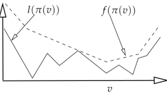
The objective of optimization–based ADP is to compute a value function v that leads to a policyπ(v)with a small policy loss l(π(v)). Unfortunately, the policy loss l◦π : (S →
R) →Ras a function of the value function lacks structure and cannot be efficiently com-puted without simulation. We, therefore, deriveupper bounds f :(S →R)→Rsuch that
v l(π(v)) f(π(v))
Figure 1.3.Optimization Framework
f ≥ lon the policy loss that are easy to evaluate and optimize, as depicted inFigure 1.3. We then develop methods that compute arg minv f as a proxy for arg minvland analyze
the error due to the proxy optimization.
Approximate linear programming (ALP), which can be classified as an optimization–based approach to ADP, has been proposed and studied previously (Schweitzer & Seidmann, 1985; de Farias, 2002). ALP uses a linear program to compute the approximate value function in a particular vector space (de Farias, 2002). ALP has been previously used in a wide variety of settings (Adelman, 2004; de Farias & van Roy, 2004; Guestrin et al., 2003). ALP has better theoretical properties than iterative approximate dynamic programming and policy search. However, theL1norm must be properly weighted to guarantee a small
policy loss, and there is no reliablemethod for selecting appropriate weights (de Farias, 2002). Among other contributions, this thesis proposes modifications of ALP that improve its performance and methods that simultaneously optimize the weights with the value function.
Value function approximation — or approximate dynamic programming — is only one of many components that are needed to solve large MDPs. Other important components are the domain samples and features — or representation — used to approximate the value function. The features represent the prior knowledge. It is desirable to develop methods that are less sensitive to the choice of the features or are able to discover them automati-cally. It is easier to specify good features for optimization–based algorithms than for itera-tive value function optimization. The guarantees on the solution quality of optimization– based methods can be used to guide feature selection for given domain samples.
The principal contribution of this thesis is the formulation and study of optimization– based methods for approximate dynamic programming. The thesis also investigates how these methods can be used for representation (feature) selection. The contributions are organized as:
1. New and improved optimization–based methods for approximate dynamic program-ming.[Part I]
(a) New bounds on the quality of an approximate value function.[Chapter 2]
(b) Lower bounds on the performance of iterative approximate dynamic program-ming.[Chapter 3]
(c) Improved formulations of approximate linear programs.[Chapter 4]
(d) Tight bilinear formulation of value function approximation.[Chapter 5]
2. Algorithms for solving optimization–based dynamic programs.[Part II]
(a) Homotopy continuation methods for solving optimization–based formulation.
[Chapter 6]
(b) Approximate algorithms for optimization–based formulations.[Chapter 7]
(c) Methods for more efficiently solving some classes of bilinear programs involved in value function approximation.[Chapter 8]
3. Methods for selecting representation. [Part III]
(a) Sampling bounds for optimization–based methods.[Chapter 9]
(b) Representation selection based on sampling bounds and the homotopy meth-ods.[Chapter 10]
4. Connections between value function approximation and classical planning. [ Chap-ter 11]
1.3 Outline
The thesis is divided into three main parts. Part Iis concerned with quality measures of approximate value functions and how to formulate them as optimization problems. The formulations are linear and nonlinear mathematical programs. In particular, Chapter 2 describes the Markov decision process framework, notation, and terms. It also defines
the crucial concepts with respect to the quality of approximate value functions. Chap-ter 3overviews the classic iterative methods for value function approximation and shows that they intrinsically cannot offer the same guarantees as optimization–based methods. Chapter 4 overviews approximate linear programming, an existing optimization–based method, and identifies key problems with the formulation. The chapter also proposes and analyzes methods for addressing these issues. Finally,Chapter 5proposes approximate bi-linear programs — a new formulation that offers the tightest possible guarantees in some instances.
The second part,Part II, then describes methods that can be used to solve the mathematical programs. These methods build on the specific properties of the formulations for increased efficiency. In particular,Chapter 6proposes a homotopy continuation method for solving approximate linear programs. This method can be used to solve very large approximate linear programs and can also be used to select the appropriate expressivity of the approx-imation features. Chapter 7 overviews the difficulties with solving approximate bilinear programs using existing methods and proposes new approximate algorithms. Because bi-linear programs are inherently hard to solve,Chapter 8describes methods that can be used to approximately solve some classes of approximate bilinear programs.
Finally,Part IIIdescribes how the proposed optimization–based techniques can be used to select and discover features in approximate dynamic programming. In particular, Chap-ter 9shows how the structure of a domain together with the structure of the samples can be used to bound the performance-loss due to insufficient domain samples. Approximate dynamic programming, and the optimization–based methods in particular, can overfit the solution if given rich sets of features. Because flexible solution methods must be able to handle rich representation spaces,Chapter 10proposes methods that can be used to auto-matically select appropriate feature composition for a given set of samples. Finally, Chap-ter 11 describes connections between approximate dynamic programming and learning heuristic functions in classical search.
A comprehensive list of all symbols used in the thesis can be found inAppendix A. Ap-pendix Bdescribes the benchmark problems used throughout the thesis. Most of the proofs
and technical properties are provided inAppendix C. Figure 1shows the significant de-pendencies between chapters and the suggested reading order. Finally, most chapters con-clude with a short summary of the contributions presented in the chapter.
PART I
CHAPTER 2
FRAMEWORK: APPROXIMATE DYNAMIC PROGRAMMING
This chapter introduces the planning framework used in this thesis. This framework is a simplification of the general reinforcement learning framework, which often assumes that the process and its model are unknown and are only revealed through acting. We, on the other hand, generally assume that samples of behavior histories are available in advance. Therefore, while some reinforcement learning algorithms interleave optimization and act-ing, we treat them as two distinct phases.
Domain samples can either come fromhistorical dataor from agenerative model. A gener-ative model can simulate the behavior of the states in a domain, but does not necessarily describe it analytically. Such generative models are often available in industrial applica-tions.
Treating the sample generation and optimization as distinct processes simplifies the anal-ysis significantly. There is no need to tradeoff exploration for exploitation. While there is still some cost associated with gathering samples, it can be analyzed independently from runtime rewards.
2.1 Framework and Notation
The thesis relies on an analysis of linear vector spaces. All vectors are column vectors by default. Unless specified otherwise, we generally assume that the vector spaces are finite-dimensional. We use1and0to denote vectors of all ones or zeros respectively of an appropriate size. The vector1i denotes the vector of all zeros excepti-th element, which is
Definition 2.1. Assume thatx ∈ Rn is a vector. A polynomial L
p norm, a weighted L1
norm, anL∞ norm, and a span seminormk · ksare defined as follows respectively:
kxkpp =
∑
i |x(i)|p kxk 1,c =∑
i c(i)|x(i)| kxk∞ =max i |x(i)| kxks=maxi x(i)−mini x(i).Span of a vector defines a seminorm, which satisfies all the properties of a norm except thatkxks=0 does not implyx =0. We also use:
[x]+=max{x,0} [x]− =min{x,0}.
The following common properties of norms are used in the thesis.
Proposition 2.2. Letk · kbe an arbitrary norm. Then:
kcxk=|c|kxk kx+yk ≤ kxk+kyk
|xTy| ≤ kxkpkyk1−1/p
|xTy| ≤ kxk1kyk∞
2.2 Model: Markov Decision Process
The particular planning model is the Markov decision process (MDP). Markov decision processes come in many flavors based on the function that is optimized. Our focus is on the infinite-horizon discounted MDPs, which are defined as follows.
Definition 2.3(e.g. (Puterman, 2005)). AMarkov Decision Processis a tuple(S,A,P,r,α).
Here,S is a finite set of states, Ais a finite set of actions, P : S × A × S 7→ [0, 1]is the transition function (P(s,a,s0)is the probability of transiting to state s0 from state s given actiona), andr : S × A 7→ R+ is a reward function. The initial distribution is: α : S 7→ [0, 1], such that∑s∈Sα(s) =1.
The goal of the work is to find a sequence of actions that maximizesγ-discounted
cumu-lative sum of the rewards, also called thereturn. A solution of a Markov decision process is a policy, which is defined as follows.
Definition 2.4. A deterministic stationarypolicyπ :S 7→ Aassigns an action to each state
of the Markov decision process. A stochastic policypolicyπ :S × A 7→[0, 1]. The set of all
stochastic stationary policies is denoted asΠ.
General non-stationary policies may take different actions in the same state in different time-steps. We limit our treatment to stationary policies, since for infinite-horizon MDPs there exists an optimalstationaryanddeterministicpolicy. We also consider stochastic poli-cies because they are more convenient to use in some settings that we consider.
We assume that there is an implicit ordering on the states and actions, and thus it is possible to represent any function onS andAas either a function, or as a vector according to the ordering. Linear operators on these functions then correspond to matrix operations. Given a policy π, the MDP turns into a Markov reward process; that is a Markov chain
with rewards associated with every transition. Its transition matrix is denoted asPπ and
represents the probability of transiting from the state defined by the row to the state de-fined by the column. For any to statess,s0 ∈ S:
Pπ(s,s0) =
∑
a∈A
P(s,s,s0)π(s,a).
The reward for the process is denoted asrπ, and is defined as:
rπ(s) =
∑
a∈A
r(s,a)π(s,a).
To simplify the notation, we use Pa to denote the stochastic matrix that represents the
transition probabilities, given a policyπ, such thatπ(s) = afor all statess ∈ S. We also
The optimization objective, or areturn, for a policyπis expressed as: Es0∼α " ∞
∑
t=0 γtr(st,at) s0 =s,a0 =π(s0), . . . ,at=π(st) # ,where the expectation is over the transition probabilities. Using the matrix notation de-fined above, the problem of fining an optimal policy can be restated as follows:
π∗ ∈arg max π∈Π ∞
∑
t=0 αT(γPπ)trπ =arg max π∈Π αT(I−γPπ)−1rπ.The equality above follows directly from summing the geometric sequence. The optimal policies are often calculated using a value function, defined below.
Avalue function v : S → R assigns a real value to each state. This may be an arbitrary function, but it is meant to capture the utility of being in a state. A value function for a policyπis defined as follows:
vπ = ∞
∑
t=0 (γPπ)trπ = (I−γPπ)− 1r πThe return for a policyπwith a value functionvπ can easily be shown to beαTvπ. The
op-timal value functionv∗is the value function of the optimal policyπ∗. The formal definition
of an optimal policy and value function follows.
Definition 2.5. A policyπ∗with the value functionv∗isoptimalif for every policyπ:
αTv∗= αT(I−γPπ∗)−1rπ∗ ≥αT(I−γPπ)−1rπ.
The basic properties of value functions and policies are described inSection 2.3.
The action-value function q : S × A 7→ R for a policy π, also known as Q-function, is
defined similarly to value function:
qπ(s,a) =r(s,a) +γ
∑
s∈S vπ(s).
An optimal action-value functionq∗is the action-value function of the optimal policy. We useq(a)to denote a subset of elements ofqthat correspond to actiona; that isq(·,a). In addition, a policyπinduces astate visitation frequency uπ :S →R, defined as follows:
uπ =
I−γPπT
−1
α.
The return of a policy depends on the state-action visitation frequencies and it is easy to show thatαTvπ = rTuπ. The optimal state-action visitation frequency isuπ∗. State-action visitation frequency u:S × A →Rare defined for all states and actions. Notice the missing subscript and that the definition is forS × Anot just states. We useua to denote the part
ofuthat corresponds to actiona ∈ A. State-action visitation frequencies must satisfy:
∑
a∈A
(I−γPπ) Tu
a =α.
2.3 Value Functions and Policies
We start the section by defining the basic properties of value functions and then discuss how a value function can be used to construct a policy. These properties are important in defining the objectives in calculating a value function. The approximate value function ˜v
in this section is an arbitrary estimate of the optimal value functionv∗.
Value functions serve to simplify the solution of MDPs because they are easier to calculate and analyze than policies. Finding the optimal value function for an MDP corresponds to finding a fixed point of thenonlinear Bellman operator(Bellman, 1957).
Definition 2.6((Puterman, 2005)). The Bellman operatorL : R|S| → R|S| and the value
function updateLπ :R|S| →R|S|for a policyπare defined as:
Lπv =γPπv+rπ Lv=max
π∈Π Lπv.
The operator L is well-defined because the maximization can be decomposed state-wise. That is Lv≥ Lπvfor all policiesπ ∈ Π. Notice thatLis anon-linear operatorandLπ is an affine operator(a linear operator offset by a constant).
A value function is optimal when it is stationary with respect to the Bellman operator.
Theorem 2.7((Bellman, 1957)). A value function v∗is optimal if and only if v∗ = Lv∗. Moreover,
v∗is unique and satisfies v∗ ≥vπ.
The proof of the theorem can be found inSection C.2. The proof of this basic property is inSection C.2. It illustrates well the concepts used in other proofs in the thesis.
Because the ultimate goal of solving an MDP is to compute a good policy, it is necessary to be able to compute a policy from a value function. The simplest method is to take the greedy policy with respect to the value function. A greedy policy takes in each state the action that maximizes the expected value when transiting to the following state.
Definition 2.8(Greedy Policy). A policyπisgreedywith respect to a value functionvwhen
π(s) =arg max a∈A r(s,a) +γs
∑
0∈S P(s,a,s0)v(s0) =arg max a∈A 1 T s (ra+γPav),and is greedy with respect to an action-value functionqwhen
π(s) =arg max
a∈A q(s,a).
The following propositions summarize the main properties of greedy policies.
Proposition 2.9. The policyπ greedy for a value-function v satisfies Lv = Lπv ≥ Lπ0v for all
policiesπ0 ∈ Π. In addition, the greedy policy with respect to the optimal value function v∗is an optimal policy.
The proof of the proposition can be found inSection C.3.
Most practical MDPs are too large for the optimal value function to be computed precisely. In these cases, we calculate an approximate value function ˜vand take the greedy policyπ
with respect to it. The quality of such a policy can be evaluated from its value functionvπ
in one of the following two main ways.
Definition 2.10(Policy Loss). Letπbe a policy computed from value function
approxima-tion. Theaverage policy lossmeasures the expected loss ofπand is defined as:
kv∗−vπk1,α =α Tv∗
−αTvπ (2.1)
Therobust policy lossmeasures the robust policy loss ofπand is defined as:
kv∗−vπk∞ =max
s∈S |v
∗(s)−v
π(s)| (2.2)
The average policy loss captures the total loss of discounted average reward when follow-ing the policyπinstead of the optimal policy, assuming the initial distribution. The robust
policy loss ignores the initial distribution and measures the difference for the worst-case initial distribution.
Taking the greedy policy with respect to a value function is the simplest method for choos-ing a policy. There are other — more computationally intensive — methods that can often lead to much better performance, but are harder to construct and analyze. We discuss these and other methods in more detail inChapter 11.
The methods for constructing policies from value functions can be divided into two main classes based on the effect of the value function error, as Chapter 11 describes in more detail. In the first class of methods, the computational complexity increases with a value function error, but solution quality is unaffected. A* and other classic search methods are included in this class (Russell & Norvig, 2003). In the second class of methods, the so-lution quality decreases with value function error, but the computational complexity is unaffected. Greedy policies are an example of such a method. In the remainder of the the-sis, we focus on greedy policies because they are easy to study, can be easily constructed, and often work well.
A crucial concept in evaluating the quality of a value function with respect to the greedy policy is the Bellman residual, which is defined as follows.
S
v−
L v v∈ K
e v∈ K
(
e)
Figure 2.1.Transitive-feasible value functions in an MDP with a linear state-space.
Definition 2.11 (Bellman residual). The Bellman residual of a value function vis a vector
defined asv−Lv.
The Bellman residual can be easily estimated from data, and is used in bounds on the policy loss of greedy policies. Most methods that approximate the value function are at least loosely based on minimization of a function of the Bellman residual.
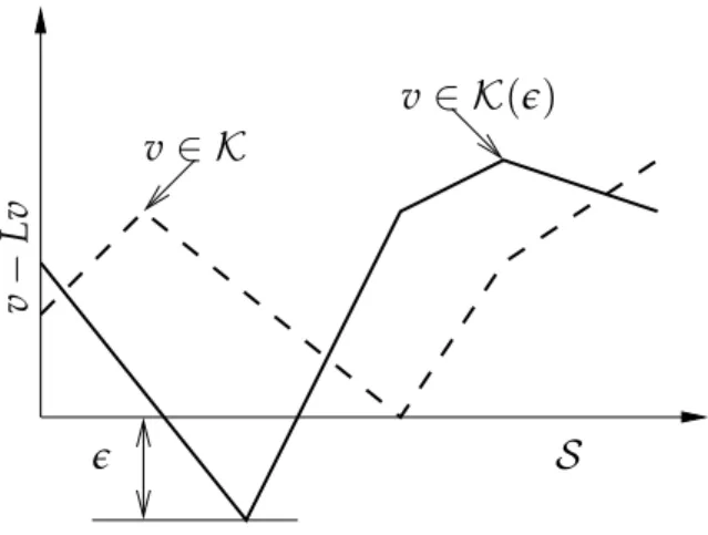
In many of the methods that we study, it is advantageous to restrict the value functions so that their Bellman residual must be non-negative, or at least bounded from below. We call such value functions transitive-feasible and define them as follows.
Definition 2.12. A value function istransitive-feasiblewhenv ≥ Lv. The set of
transitive-feasible value functions is:
K ={v∈R|S| v≥ Lv}.
Assume an arbitrary e ≥ 0. The set of e-transitive-feasible value functions is defined as
follows:
K(e) ={v ∈R|S| v≥ Lv−e1}.
Notice that the optimal value functionv∗is transitive-feasible, which follows directly from Theorem 2.7. Transitive-feasible value functions are illustrated inFigure 2.1. The following lemma summarizes the main importance of transitive-feasible value functions:
Lemma 2.13. Transitive feasible value functions are an upper bound on the optimal value function. Assume ane-transitive-feasible value function v∈ K(e). Then:
v≥v∗− e
1−γ1.
The proof of the lemma can be found inSection C.2.
Another important property of transitive-feasible value functions follows.
Proposition 2.14. The set K of transitive-feasible value functions is convex. That is for any
v1,v2∈ Kand anyβ∈[0, 1]also βv1+ (1−β)v2 ∈ K.
The proof of the proposition can be found inSection C.2.
The crucial property of approximate value functions is the quality of the corresponding greedy policy. The robust policy loss can be bounded as follows.
Theorem 2.15. Letv be the approximate value function, and v˜ πbe a value function of an arbitrary
policyπ. Then: kv∗−vπk∞ ≤ 1 1−γkv˜−Lπv˜k∞+kv˜−v ∗k ∞ kv∗−vπk∞ ≤ 2 1−γkv˜−Lπv˜k∞
The proof of the theorem can be found inSection C.3. This theorem extends the classical bounds on policy loss (Williams & Baird, 1994). The following theorem states the bounds for the greedy policy in particular.
Theorem 2.16(Robust Policy Loss). Letπbe the policy greedy with respect tov. Then:˜
kv∗−vπk∞ ≤
2
1−γkv˜−Lv˜k∞.
In addition, ifv˜ ∈ K, the policy loss is minimized for the greedy policy and:
kv∗−vπk∞ ≤
1
1−γkv˜−Lv˜k∞.
The proof of the theorem can be found inSection C.3.
The bounds above ignore the initial distribution. When the initial distribution is known, bounds on the expected policy loss can be used.
Theorem 2.17(Expected Policy Loss). Letπbe a greedy policy with respect to a value function
˜
v and let the state-action visitation frequencies ofπbe bounded as u≤uπ ≤u. Then:¯
kv∗−vπk1,α =α Tv∗
−αTv˜+uπT(v˜−Lv˜)
≤αTv∗−αTv˜+uT[v˜−Lv˜]−+u¯T[v˜−Lv˜]+.
The state-visitation frequency uπdepends on the initial distributionα, unlike v∗. In addition, when
˜
v∈ K, the bound is:
kv∗−vπk1,α ≤ −kv∗−v˜k1,α+kv˜−Lv˜k1, ¯u
kv∗−vπk1,α ≤ −kv∗−v˜k1,α+
1
1−γkv˜−Lv˜k∞
The proof of the theorem can be found inSection C.3. The proof is based on the com-plementary slackness principle in linear programs (Mendelssohn, 1980; Shetty & Taylor, 1987; Zipkin, 1977). Notice that the bounds inTheorem 2.17can be minimized even with-out knowingv∗. The optimal value functionv∗ is independent of the approximate value function ˜vand the greedy policyπdepends only on ˜v.
Remark2.18. The bounds inTheorem 2.17generalize the bounds of Theorem 1.3 in (de Farias, 2002). Those bounds state that wheneverv ∈ K:
kv∗−vπk1,α ≤
1 1−γkv
∗−v˜k
1,(1−γ)u.
This bound is a special case ofTheorem 2.17because:
kv˜−Lv˜k1,u≤ kv∗−v˜k1,u ≤
1 1−γkv
∗−v˜k
1,(1−γ)u,
fromv∗ ≤ Lv˜ ≤v˜andαTv∗−αTv˜ ≤0. The proof ofTheorem 2.17also simplifies the proof
of Theorem 1.3 in (de Farias, 2002)
The bounds from the remark above can be further tightened and revised as the following theorem shows. We use this new bound later to improve the standard ALP formulation.
Theorem 2.19(Expected Policy Loss). Letπbe a greedy policy with respect to a value function
˜
v and let the state-action visitation frequencies ofπbe bounded as u≤uπ ≤u. Then:¯
kv∗−vπk1,α ≤ ¯ uT(I−γP∗)−αT (v˜−v∗) +u¯T[Lv˜−v˜]+,
where P∗= Pπ∗. The state-visitation frequency uπdepends on the initial distributionα, unlike v∗. In addition, whenv˜∈ K, the bound can be simplified to:
kv∗−vπk1,α ≤u¯ T(I
−γP∗)(v˜−v∗) This simplification is, however, looser.
The proof of the theorem can be found inSection C.3.
Notice the significant difference between Theorems2.19and2.17. Theorem 2.19involves the term[Lv˜−v˜]+, while inTheorem 2.17it is reversed to be ˜v−[Lv˜]+.
The bounds above play in important role in the approaches that we propose. Chapter 4 shows that approximate linear programming minimizes bounds on the expected policy
loss in Theorems 2.17and2.19. However, it only minimizes loose upper bounds. Then, Chapter 5shows that the tighter bounds on Theorems2.17and2.16can be optimized using approximate bilinear programming.
2.4 Approximately Solving Markov Decision Processes
Most interesting MDP problems are too large to be solved precisely and must be approxi-mated. The methods for approximately solving Markov decision processes can be divided into two main types: 1) policy search methods, and 2) approximate dynamic programming
methods. This thesis focuses on approximate dynamic programming.
Policy search methods rely on local search in a restricted policy space. The policy may be represented, for example, as a finite-state controller (Stanley & Miikkulainen, 2004) or as a greedy policy with respect to an approximate value function (Szita & Lorincz, 2006). Policy search methods have achieved impressive results in such domains as Tetris (Szita & Lorincz, 2006) and helicopter control (Abbeel et al., 2006). However, they are notoriously hard to analyze. We are not aware of any theoretical guarantees regarding the quality of the solution.
Approximate dynamic programming (ADP) methods, also known as value function ap-proximation, first calculate the value function approximately (Bertsekas & Ioffe, 1997; Powell, 2007a; Sutton & Barto, 1998). The policy is then calculated from this value function. The advantage of value function approximation is the it is easy to determine the quality of a value function using samples, while determining a quality of a policy usually requires extensive simulation. We discuss these properties in greater detail inSection 2.3.
A basic setup of value function approximation is depicted inFigure 2.2. The ovals repre-sent inputs, the rectangles reprerepre-sent computational components, and the arrows reprerepre-sent information flow. The input “Features” represents functions that assign a set of real val-ues to each state, as described in Section 2.4.1. The input “Samples” represents a set of simple sequences of states and actions generated using the transition model of an MDP, as described inSection 2.4.2.
Calculate value
function
Compute policy
Value function
Execute policy
Policy
Offline
Online: samples
Features
Samples
Figure 2.2.Approximate Dynamic Programming Framework.
A significant part of the thesis is devoted to studying methods that calculate the value function from the samples and state features. These methods are described and analyzed in Chapters3,4, and5. A crucial consideration in the development of the methods is the way in which a policy is constructed from a value function.
Value function approximation methods can be classified based on the source of samples intoonlineandofflinemethods asFigure 2.2shows. Online methods interleave execution of a calculated policy with sample gathering and value function approximation. As a re-sult, a new policy may be often calculated during execution. Offline methods use a fixed number of samples gathered earlier, prior to plan execution. They are simpler to analyze and implement than online methods, but may perform worse due to fewer available sam-ples. To simplify the analysis, our focus is on the offline methods, and we indicate the potential difficulties with extending the methods to the online ones when appropriate.
2.4.1 Features
The set of the state features is a necessary component of value function approximation. These features must be supplied in advance and must roughly capture the properties of the problem. For each states, we define a vectorφ(s)of features and denoteφi :S →Rto
be a function that maps states to the value featurei:
φi(s) = (φ(s))i.
The desirable properties of features to be provided depend strongly on the algorithm, sam-ples, and attributes of the problem, and their best choice is not yet fully understood. The feature functionφican also be treated as a vector, similarly to the value functionv. We use
|φ|to denote the number of features.
Value function approximation methods combines the features into a value function. The main purpose is to limit the possible value functions that can be represented, as the fol-lowing shows.
Definition 2.20. Assume a givenconvexpolyhedral set M ⊆ R|S|. A value functionvis
representable(inM) ifv∈ M.
This definition captures the basic properties and we in general assume its specific instanti-ations. In particular, we generally assume thatMcan be represented using a set of linear constraints, although most approaches we propose and study can be easily generalized to quadratic functions.
Many complex methods that combine features into a value function have been developed, such as neural networks and genetic algorithms (Bertsekas & Ioffe, 1997). Most of these complex methods are extremely hard to analyze, computationally complex, and hard to use. A simpler, and more common, method islinear value function approximation. In linear value function approximation, the value function is represented as a linear combination of
nonlinear featuresφ(s). Linear value function approximation is easy to apply and analyze,
It is helpful to represent linear value function approximation in terms of matrices. To do that, let the matrixΦ: |S| ×mrepresent the features, wheremis the number of features. The feature matrixΦ, also known asbasis, has the features of the statesφ(s)as rows:
Φ= − φ(s1)T − − φ(s2)T − .. . Φ= | | φ1 φ2 . . . | |
The value functionvis then represented asv=ΦxandM =colspan(Φ)
Generally, it is desirable that the number of all features is relatively small because of two main reasons. First, a limited set of features enables generalization from an incomplete set of samples. Second, it reduces computational complexity since it restricts the space of rep-resentable value functions. When the number of features is large, it is possible to achieve these goals usingregularization. Regularization restricts the coefficientsxinv =Φxusing a norm as:kxk ≤ψ. Therefore, we consider the following two types of representation:
Linear space: M={v∈R|S| v=Φx}
Regularized: M(ψ) = {v ∈ R|S| v = Φx, Ω(x) ≤ ψ}, whereΩ : Rm → R is aconvex
regularization function andmis the number of features.
When not necessary, we omitψin the notation ofM(ψ). Methods that we propose require
the following standard assumption (Schweitzer & Seidmann, 1985).
Assumption 2.21. All multiples of the constant vector 1are representable inM. That is,
for allk∈Rwe have thatk1∈ M.
We implicitly assume that the first column of Φ— that is φ1 — is the constant vector 1.
Assumption 2.21is satisfied when the first column ofΦis1— or a constant feature — and the regularization (if any) does not place any penalty on this feature. The influence of the constant features is typically negligible because adding a constant to the value function does not influence the policy asLemma C.5shows.
s1 s2 a1 (s2,a1) (s1,a2) (s1,a1) a1 a2
Figure 2.3.Example of equivalence of pairs of state-action values.
The state-action value function qcan be approximated similarly. The main difference is that the functionqis approximated for all actionsa∈ A. That is for all actionsa∈ A:
q(a) =Φaxa.
Notice thatΦaandxamay be the same for multiple states or actions.
Policies, like value functions, can be represented as vectors. That is, a policy π can be
represented as a vectors over state-action pairs.
2.4.2 Samples
In most practical problems, the number of states is too large to be explicitly enumerated. Therefore, even though the value function is restricted as described in Section 2.4.1, the problem cannot be solved optimally. The approach taken in reinforcement learning is to sample a limited number of states, actions, and their transitions to approximately calculate the value function. It is possible to rely on state samples because the value function is restricted to the representable setM. Issues raised by sampling are addressed in greater detail inChapter 9.
Samples are usually used to approximate the Bellman residual. First, we show a formal definition of the samples and then show how to use them.
Definition 2.22. One-step simple samplesare defined as:
˜
˜
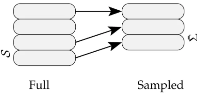
Σ Σ¯
Figure 2.4.Sample types
wheres1. . .snare selected i.i.d. from the distributionP(s,a)forevery s,a independently.
Definition 2.23. One-step samples with expectationare defined as follows:
¯
Σ⊆ {(s,a,P(s,a),r(s,a)) s∈ S, a∈ A}.
Notice that ¯Σare more informative than ˜Σ, but are often unavailable. Membership of states in the samples is denoted simply ass ∈Σor(s,a)∈Σwith the remaining variables, such asr(s,a)considered to be available implicitly. Examples of these samples are sketched in Figure 2.4.
We use|Σ¯|sto denote the number of samples in terms of distinct states, and|Σ¯|ato denote
the number of samples in terms of state–action pairs. The same notation is used for ˜Σ. As defined here, the samples do not repeat for states and actions, which differs from the traditional sampling assumptions in machine learning. Usually, the samples are assumed to be drawn with repetition from a given distribution. In comparison, we do not assume a distribution over states and actions.
The sampling models vary significantly in various domains. In some domains, it may be very easy and cheap to gather samples. In the blood inventory management problem, the model of the problem has been constructed based on historical statistics. The focus of this work is on problems with a model available. This fact simplifies many of the assumptions on the source and structure of the samples, since they can be essentially generated for an arbitrary number of states. In general reinforcement learning, often the only option is to gather samples during the execution. Much work has focused on defining setting and
sample types appropriate in these settings (Kakade, 2003), and we discuss some of them inChapter 9.
Inonlinereinforcement learning algorithms (seeFigure 2.2), the samples are generated dur-ing the execution. It is important then to determine the tradeoff between exploration and exploitation. We, however, considerofflinealgorithms, in which the samples are generated in advance. While it is still desirable to minimize the number of samples needed there is no tradeoff with the final performance. Offline methods are much easier to analyze and are more appropriate in many planning settings.
The samples, as mentioned above, are used to approximate the Bellman operator and the set of transitive-feasible value functions.
Definition 2.24. Thesampled Bellman operatorand the corresponding set of sampled
transitive-feasible functions are defined as:
(L¯(v))(s¯) = max{a (s¯,a)∈Σ¯}r(s¯,a) +γ∑s0∈SP(s¯,a,s0)v(s0) when ¯s∈ Σ¯ −∞ otherwise (2.3) ¯ K= {v ∀s∈ S v(s)≥ (Lv¯ )(s)} (2.4)
The less-informative ˜Σcan be used as follows.
Definition 2.25. The estimated Bellman operator and the corresponding set of estimated
transitive-feasible functions are defined as:
(L˜(v))(s¯) = max{a (s¯,a)∈Σ˜}r(s¯,a) +γn1∑ni=1v(si) when∀s¯∈Σ˜ −∞ otherwise (2.5) ˜ K= v ∀s∈ S v(s)≥(Lv˜ )(s) (2.6)
Notice that operators ˜Land ¯L map value functions to a subset of all states — only states that are sampled. The values for other states are assumed to beundefined.
The samples can also be used to create an approximation of the initial distribution, or the distribution of visitation-frequencies of a given policy. The estimated initial distribution ¯α
is defined as: ¯ α(s) = α(s) s∈Σ¯ 0 otherwise
Although we define above the sampled operators and distributions directly, in applica-tions only their estimated versions are typically calculated. That means calculating ¯αTΦ
instead of estimating ¯αfirst. The generic definitions above help to generalize the analysis
to various types of approximate representations.
To define bounds on the sampling behavior, we propose the following assumptions. These assumptions are intentionally generic to apply to a wide range of scenarios. Chapter 9 examines some more-specific sampling conditions and their implications in practice. Note in particular that the assumptions apply only to value functions that are representable. The first assumption limits the error due to missing transitions in the sampled Bellman operator ¯L.
Assumption 2.26(State Selection Behavior). The representable value functions satisfy for
someep:
K ∩ M ⊆K ∩ M ⊆ K¯ (ep)∩ M.
WhenM(ψ)is a function ofψthen we writeep(ψ)to denote the dependence.
The constantepbounds the potential violation of the Bellman residual on states that are not
provided as a part of the sample. In addition, all value functions that are transitive-feasible for the full Bellman operator are transitive-feasible in the sampled version; the sampling only removes constraints on the set.
The second assumptions bounds the error due to sampling non-uniformity.
Assumption 2.27(Uniform Sampling Behavior). For all representable value functionsv∈
M:
|(α−α¯)Tv| ≤ec.