An approach for the impact feature extraction method based on improved modal decomposition and singular value analysis

This is a repository copy of An approach for the impact feature extraction method based on improved modal decomposition and singular value analysis.

White Rose Research Online URL for this paper: http://eprints.whiterose.ac.uk/142256/

Version: Accepted Version

Article:

Bie, F., Horoshenkov, K.V. orcid.org/0000-0002-6188-0369, Qian, J. et al. (1 more author) (2019) An approach for the impact feature extraction method based on improved modal decomposition and singular value analysis. Journal of Vibration and Control, 25 (5). pp. 1096-1108. ISSN 1077-5463

https://doi.org/10.1177/1077546318811410

Bie, F., Horoshenkov, K. V., Qian, J., & Pei, J. (2019). An approach for the impact feature extraction method based on improved modal decomposition and singular value analysis. Journal of Vibration and Control, 25(5), 1096–1108. Copyright © 2018 The Authors. https://doi.org/10.1177/1077546318811410

[email protected] https://eprints.whiterose.ac.uk/ Reuse

Items deposited in White Rose Research Online are protected by copyright, with all rights reserved unless indicated otherwise. They may be downloaded and/or printed for private study, or other acts as permitted by national copyright laws. The publisher or other rights holders may allow further reproduction and re-use of the full text version. This is indicated by the licence information on the White Rose Research Online record for the item.

Takedown

If you consider content in White Rose Research Online to be in breach of UK law, please notify us by

An approach of the impact feature extraction method based

on improved modal decomposition and singular value

analysis

Fengfeng Bie

1

_,

_{Kirill V. Horoshenkov}

2

_,

_{Jin Qian}

1

_{and Junfeng Pei}

1

Abstract

For non-stationary vibration useful information of impact feature tends to be

overwhelmed with strong routine components, which make it difficult to implement pattern recognition. This paper proposes improved signal processing methods of variational mode decomposition (VMD) and singular value decomposition (SVD) for non-stationary impact feature extraction in application to condition monitoring of reciprocating machinery. The impact feature is firstly simulated with the dynamics analysis of the driving mechanism of a reciprocating pump. Through comparison the merit of the improved VMD method is demonstrated. The singular value of the

decomposed modes is extracted with SVD method. The support vector machine method is used as the classifier for the extracted set of features. The performance of the proposed VMD-based method is validated practically through a set of measured data from the reciprocating pump setup.

Keywords

Reciprocating machinery; impact feature; Variational Mode Decomposition; singular value; pattern recognition

1. Introduction

In reciprocating machinery condition monitoring impact features are the main indicator of the non-stationary faults (Yang et al., 2010;Bolaers et al., 2011). Most of the

traditional analysis methods lose the efficiency owing to their boundedness on the feature extraction and pattern recognition (Kostyukov et al. 2016; El-ghamry et al. 2010). Signal decomposition methods have been developed in vibration analysis, in which the original vibration signal is been composed into several constituent components so that the key feature characteristics can be extracted to make them more apparent (Wang et al, 2015; Cui et al.,2009). A majority of the popular time-frequency analysis methods developed for the nonstationary signal with time-varying frequencies, such as Wavelet Transform (WT) and STFT (Auger et al.,1995; Jurado et al., 2002), Wigner–Ville (Ghofrani et al., 2009) and others (Loughlin and Davidson, 2001; Baccigalupi and Liccardo, 2016) are based on the assumption that the signal of impact feature can be accurately expressed as the sum of a number of base functions which are assumed known a priori. In these

1

School of Mechanical Engineering, Changzhou University, Changzhou 213164, China

2

Department of Mechanical Engineering, The University of Sheffield, Sheffield S1 3JD, UK

Corresponding author:

Fengfeng Bie, School of Mechanical Engineering, Changzhou University, Changzhou 213161, China E-mail address: [email protected]

methods the signal is effectively constrained to match the model definition, rendering occasional difficulty in the process of selecting the useful (usually faint) feature from the estimating or updating the fundamental frequency in the data.

The method of Empirical Mode Decomposition (EMD) is an alternative to the above time-frequency analysis methods. It was developed at the end of last century (Huang et al., 1998; Zhang et al., 2017) and become popular because its flexibility in terms of the functional basis. The EMD is based on the Intrinsic Mode Functions (IMFs) which are estimated in the recursive sifting process to represent the key features of the vibration pattern more accurately. It has been tested effectively when applied to represent a single fault mode process or stationary vibration pattern, while the mode overlap tends to occur due to its sensibility on the disturbing instantaneous frequencies for the signal of the reciprocating machinery. Another improved method of Variational Mode Decomposition (VMD) was also developed with its analytical theory framework and self-adaptive characteristics for spaced mode decomposition (Dragomiretskiy and Zosso, 2014). It was shown that the VMD method works well to extract closely spaced modes from stationary signals recorded on rotating machinery (Yue et al.,2016). However, for practical

vibration signals from reciprocating machinery, which are not necessarily stationary with the internal impacting feature, the successful applications of this method have remained problematic (McNeil, 2016).

The purpose of this paper is to study the performance of the EMD and VMD in combination with a popular classification method based on support vector machines aiming at the impact feature analysis for the reciprocating machinery. The paper is organized in the following manner. Section 2 is the theoretical foundation. Section 3 illustrates the dynamics and simulation process on the impact feature analysis, where the proposed method is basically verified on the driven mechanism of reciprocating

machinery. The results and discussions of the proposed method applied in the typical modes of reciprocating machinery are finally presented in Section 4 which is followed by the Conclusions section.

2. Theoretical foundation

2.1. Empirical mode decomposition

Let us assume that S(t) is a vibration acceleration signal recorded on a reciprocating machine and that this signal can be expressed as a combination of a set of periodic functions. Instead of using a traditional spectral analysis method, e.g. the Fourier

analysis, we will use the EMD method which is a decomposition of the signal, S(t) into a set of the Intrinsic Mode Function (IMF) components. This decomposition is based on the concept of mono-components from which the instantaneous amplitude and frequency (Baccigalupi and Liccardo, 2016; Huang et al., 1998) can be derived. This decomposition is a repetitive sifting process of seeking for the mode components, C_i(t), in the original data, S(t), until the midterm residual component,r_i(t), is relatively small. The

decomposition of the original vibration signal is then a sum of several IMF components, )

(t

C_i , and the final residual r_n(t):

) ( ) ( ) ( 1 t r t C t S _n n i i + =

∑

= . (1)

It is then common to deal with the analytic form for C_i(t), i.e.: ( )

( ) ( ) ( ) ( ) ji t

i i i i

Z t =C t + jH t =A t eθ (2) where H t_i( ) is the Hilbert transform of C t_i( ):

( ) 1 ( ) i i C H t d t τ τ π τ +∞ −∞ = −

∫

. (3) In the above equationsA t_i( ) is the amplitude function,

θ

_i( )t is the phase function and

1

j= − . Then the instantaneous pulsation ω_i can be defined as

( ) i i d t dt θ ω = (4) Virtually, the decomposition process of local wave functions could be considered as wave filtering when the practical signal was decomposed into components with frequency series of high to low.

2.2. Basic principle of VMD

Similarly to the EMD, the VMD algorithm works by decomposing the original signal,

) (t

S , into mode series (IMFs or sub-signals) with a limited frequency bandwidth. As a result, each mode k is required to be compact around a central frequency

ω

_k, which is used to determine the decomposition. The VMD algorithm is used to estimate the bandwidth of a signal as follows:

(1) For each modeu_k, the Hilbert transform is used to obtain the narrow band spectrum. (2) For each mode, the frequency of the spectral band is changed by the mixed

exponential tuned to the respectively estimated center frequency.

(3) The bandwidth is preliminarily estimated by the Gauss method, for example, the square of the L2-norm gradient. Then, a constrained variational approach (Dragomiretskiy and Zosso, 2014) is applied to estimate the IMF, u : _k

} )] ( * ) ) ( [( { min 2 ,

∑

− + ∂ = k t j k t u k k k e t u t j t ω ω δ π 5 with

∑

= k k S t u ( , ) 6 where δ is the delta-function, tis the time, t is the time derivative, and denotes the convolution. Effectivelyu_k(t)represents the IMFs decomposed through the VMD and represents central frequency series of the IMFs.

In order to achieve the desired unconstrained arguments, the following augmented Lagrange function introduced as follows:

L({ }, { }, ) = δ ( ) + ( ) + S( ) ( ) +

( )S( ) ( ) , 7 where denotes the balancing parameter of the data fidelity constraint and the

Lagrangian multiplier is a common way of enforcing constraints strictly (Jiang et al., 2016).

With the detailed saddle point of the above augmented Lagrange function, the

decomposition procedure for the original signal is then accomplished. The detailed VMD algorithm can be found in (Dragomiretskiy and Zosso, 2014).

2.3. Implementation of VMD with Singular Value Decomposition 2.3.1. Crucial arguments in the implementation

Although the VMD algorithm and EMD are both rely on a similar sifting implementation, the algorithms are based on different theoretical framework.

Specifically, the number of the IMF modes of the EMD is definite with the preset value for the final residual being the stoppage criterion. This criterion is not specified in the VMD. The evaluating method for the frequency domain analysis of the IMFs in the EMD is totally different to the way the central frequencies are estimated in the case of the VMD. The latter depends on the maximum value of k (Dragomiretskiy and Zosso, 2014) so that to the correct assignment of k is a key problem fumbled with the experience in practical cases.

In this paper, the number of the IMFs from both methods are studied on the dynamics simulation signal. It is definite as the tendency component figured out with the EMD method, while it can only be sought out with the vanishing of overlap effect among the modes. In this section the central frequency could be the crucial indicator, which is estimated respectively on the unilateral frequency spectrum from the Hilbert transform of each IMF mode.

Another aided parameter for the decomposition process is the correct assignment of the balancing parameter

α

in Eq. (7). It has been found that the value of

α

may render quite different mode components for the original impacting signals. The smaller this parameter, the greater the bandwidth of the IMF component, and vice versa - the smaller the bandwidth of the component signal. In former studies, it is found that a bigger

α

is suitable for low-frequency component (e.g., trend term) detection since the important part of distinctive spectrum would be share by the adjacent modes which may render overlaps, as the result the value of k is also be affected (Mohanty, et al. 2014). A smaller

α

is sensitive on feature variation though the part of the decomposition modes may contains extra noise, it is comparably effective in detecting the impacting feature from vibration signal. Thus, for the decomposition,

α

is set a comparably smaller one in the preliminary study from the beginning with the gradual adjusting in the procedure as an aided

reference. Since the default balancing (fidelity) parameter is 2000, the value of

α

is set as 1000 manually in view of the cross affection between the value of K and

α

in the decomposition procedure.

2.3.2. Singular value extraction and classification

With the modes from the EMD/VMD processing, the original signal is decomposed into a digital matrix that may remain unrecognizable. In order to describe the matrix character with the orthogonality of eigenvectors of the matrix remained, a lower-ranked transformation is needed. To achieve this, the Singular Value Decomposition (SVD) is applied. While for the recognizing the IMFs from the decomposition, the singular value would be introduced in the analysis of the matrixA with the IMF data.

The process can be described as follows. We assume that A is an n×d matrix with n

corresponding singular values , , … , . The matrix A can be decomposed into a sum of rank one matrices as (Rockfellar, 1973)

A = U V,

8 where U V, are the matrices with left-singular and right singular vectors, respectively, and is the diagonal matrix with the singular values σ σ1, 2,...,σr. In this way, the IMF

matrix can be characterized by the distinctive singular vectors and corresponding singular values which are useful for the purpose of condition classification. With the singular value group employed as the distinctive parameters in this paper, the largest one could be chosen as the depiction of the research object.

In order to realize the final pattern recognition from the singular value, the Support Vector Machine (SVM) learner (Vapnik, 1995; Zanaty, 2012) is employed as a classifier for singular values , , … , of A as the final step. The SVM learner is trained with a

training dataset. The main purpose of the learner is to find an optimal segmentation of the hyper plane from the input singular value matrix by constructing the classification hyper plane, the two classes are separated and the maximum classified spaces of the two kinds are obtained effectively with the assigned-kernel SVM algorithm.

2.4. Procedure of the proposed method

In summary, the pattern recognition procedure of the proposed method is shown schematically in Figure 1. The method is studied in two stages: on the simulated vibration signal and on real data. The dynamics simulation is used to study the performance of the two decomposition methods. At this stage the arguments of k and are optimized to improve the quality of the VMD method in application to the simulated data. Then the singular value of the modes from the decomposition is achieved by SVD, and the pattern recognition from the SVM classification shows that the VMD-based method is effective for single fault mode recognition from the normal. The second stage is the experimental validation of the VMD-based method on practical testing vibration signals from an experiment on reciprocating machinery. At this stage the improved VMD-based method is applied to extract the singular value from the IMFs with the SVD technique to use as the consequent input of the SVM classification for the ultimate pattern recognition.

Figure 1. An illustration of the EMD/VMD-SVD analysis procedure.

3. Dynamics simulation and preliminary analysis

3.1. Dynamics analysis and simulation

Collect original vibration signal

Time-frequency domain analysis Improved VMD and implementation

Extracting singular value

Pattern recognition with SVM classification Approach of EMD and VMD with dynamics simulation

As the preliminary study for the proposed method, the comparison between EMD and VMD is implemented here in a typical reciprocating mechanism with a distinctive impacting feature configurated through the simulation system. In a typical reciprocating mechanism, e.g. 3NB-1300 slurry pump shown schematically in Figure 2, the

relationship between the crank angle, and the displacement, velocity and acceleration of the driven end of the pump are known and were used in this work (Ranjbarkohan et al., 2011; Jomartov et al.,2015). In the dynamics simulation process specified parameters were stiffness coefficient, force exponents, damping and penetration depth of the kinematic pairs in the Automatic Dynamic Analysis of Mechanical Systems (ADAMS) modelling tool. First of all, the motion of the key components of crankshaft was

simulated with the given dimensions of crankshaft (diameter of 42mm ) and connection rod (length of 236mm), the equation of the d (displacement), v (velocity) and a

(acceleration) with the variation of the angle is:

d = R[(n + 1) cos (sin ) ] 9 v = R[sin + [ ( ) ] / ] 10 a = [cos + [ ( ) ] + [ ( ) ] / ] 11

where R is the diameter of the crank, L is the length of the rod, and n = .

Figure 2. Fault simulated by the imposed force on the first bush-shaft assembly.

Figure 3. The parameters of the crankshaft parts as a function of the angle.

0 1 2 3 4 5 6 Angle -10 -5 0 5 10 15 Parameter- d,v,a

crankshaft dynamics parameter contrast

displacement velocity acceleration Force location applied on the first bush

Connection rod

For the later, the impact load F is applied on the bearing bush as designed according to the maximum value of ain equation (11), which is illustrated in Figure 2.With the dynamics analysis as shown in Figure 3, the acceleration signal is more sensible in reflecting the system deformation caused by impacting forces. Two typical conditions for the crankshaft connecting-journal bearing were simulated: normal and fault. In this fault arrangement, the abnormal impact load is set on the first bush-shaft assembly, which is precisely simulated with the constrain parameters of the system configuration.

In the model, the crankshaft, connecting rod, piston and pin according to the real dimension of the pump mechanism were set with the specified constrains, including the stiffness coefficient, force exponent, damping and penetration depth of the contacting surface of crankshaft and bearing bush. Among these parameters in the configuration, the stiffness is the basic and most influential one for the impacting force which leads to most of the rotating faults. In the practical force simulation, the value of force exponent rests upon the material of the parts, the damping coefficient relies on the set of the stiffness, and the penetration depth needs to be manually selected according to the actual

restrictions.

In order to simulate the applied impacting force specifically, the stiffness coefficient was set according to:

* 2 1 3 4 E R K = (12) where 2 1 1 1 1 R R R = +

, and are the radii of the two colliding parts, and

2 2 2 1 2 1 * 1 1 1 E E E υ υ ₊ − −

= , ν₁ and ν₂ are the respective Poisson’s ratio, and as the

respective elasticity modulus. The force exponent of the metal-metal is set as 1.5. The maximum damping coefficient is set as 1% of the stiffness for the energy loss simulation, and the penetration depth is defined as the invasion between both colliding interfaces, which is optimized subjecting to the permissible damping and finally chosen as the default value of 0.1mm.

3.2. Impact character simulation

With the dynamic simulation of targeted configuration, a series of acceleration signals from the crankshaft vibration are obtained. The time and frequency domain of the typical vibration signals are shown in Figure 4 and 5 respectively, which illustrates that the cyclical impact with different magnitudes of the reciprocating machinery is embodied in two typical conditions of normal and fault mode. In particular, the impacting features caused by the abnormal force on the bush are added to the simulated fault mode as shown in time domain signal. We can also find some difference in the spectrum distribution of the two approximately from 500Hz to 1500Hz as shown in Figure 5.In order to basically testify the VMD-SVM model for the impacting feature extraction in the simulation stage, the contrast of EMD and VMD on the signals with the SVM classifier are achieved individually.

Figure 4. Acceleration time domain signal of normal (left) and fault (right) status.

Figure 5. Spectrum of normal (left) and fault (right) status.

The EMD and VMD methods were applied to the data of both conditions. In the VMD decomposition process, the value of kwas not defined until the central frequency of the adjacent two modes come out as similar in avoiding the over decomposition (overlap). Since IMF6 and IMF7 are found to contain similar central frequencies here, the number of the IMF was set to k = 6 in this analysis. The signal decomposition is shown in Figure 6 for the normal and fault conditions. In view of the overall distinction between the decompositions of the two methods, we can find that the impact feature of the vibration involved in the time domain signal is mostly embodied in the main IMFs other than the high orders and tendency component, therefore the first 6 IMFs of EMD are selected as the analysis object. In the contrast of the decomposition results of EMD, we can find that VMD can adaptively decompose the simulated signal into a succinct ensemble of

intrinsic mode functions of specialized bands with the given k, which is more efficient and suitable for the following feature recognition.

0 0.1 0.2 0.3 0.4 0.5 0.6 0.7 0.8 0.9 1 Time(s) -0.15 -0.1 -0.05 0 0.05 0.1 0.15 Amplitude(g) 0 0.2 0.4 0.6 0.8 1 Time(s) -1 -0.75 -0.5 -0.25 0 0.25 0.5 0.75 1 Amplitude(g) 0 500 1000 1500 2000 Frequency (Hz) 0 0.01 0.02 0.03 0.04 0.05 Amplitude (g) 0 500 1000 1500 2000 Frequency(Hz) 0 0.02 0.04 0.06 0.08 0.1 0.12 Amplitude(g)

a. Decomposition of VMD

b. Decomposition of EMD

Figure 6. Signal decomposition for the fault simulation (left as normal, right as fault).

Each of the characteristic vector of each decomposition signal is characterized by singular value which is shown in Table 1. Compared with the normal conditions, the achieved singular value varies greatly with VMD method (when k = 1), illustrates that the magnitude of the VMD IMFs reflect the feature of the signal more saliently. As

0 0.1 0.2 0.3 0.4 0.5 -0.2 0 0.2 0 0.1 0.2 0.3 0.4 0.5 -0.2 0 0.2 0 0.1 0.2 0.3 0.4 0.5 -0.2 0 0.2 0 0.1 0.2 0.3 0.4 0.5 -0.2 0 0.2 0 0.1 0.2 0.3 0.4 0.5 -0.5 0 0.5 0 0.1 0.2 0.3 0.4 0.5 Time -0.2 0 0.2 Amplitude of IMFs 0 0.1 0.2 0.3 0.4 0.5 -0.5 0 0.5 0 0.1 0.2 0.3 0.4 0.5 -1 0 1 0 0.1 0.2 0.3 0.4 0.5 -1 0 1 0 0.1 0.2 0.3 0.4 0.5 -0.5 0 0.5 0 0.1 0.2 0.3 0.4 0.5 -0.5 0 0.5 0 0.1 0.2 0.3 0.4 0.5 Time -0.5 0 0.5 Amplitude of IMFs 0 0.05 0.1 0.15 0.2 0.25 0.3 0.35 -0.5 0 0.5 0 0.05 0.1 0.15 0.2 0.25 0.3 0.35 -0.2 0 0.2 0 0.05 0.1 0.15 0.2 0.25 0.3 0.35 -0.2 0 0.2 0 0.05 0.1 0.15 0.2 0.25 0.3 0.35 -0.05 0 0.05 0 0.05 0.1 0.15 0.2 0.25 0.3 0.35 -0.05 0 0.05 0 0.05 0.1 0.15 0.2 0.25 0.3 0.35 -0.05 0 0.05 0 0.05 0.1 0.15 0.2 0.25 0.3 0.35 -0.02 0 0.02 0 0.05 0.1 0.15 0.2 0.25 0.3 0.35 -0.02 0 0.02 0 0.05 0.1 0.15 0.2 0.25 0.3 0.35 -5 0 5 10 -3 0 0.05 0.1 0.15 0.2 0.25 0.3 0.35 Time -5 0 5 Amplitude of IMFs 10-3 0 0.1 0.2 0.3 0.4 0.5 0.6 0.7 0.8 0.9 1 -2 0 2 0 0.1 0.2 0.3 0.4 0.5 0.6 0.7 0.8 0.9 1 -1 0 1 0 0.1 0.2 0.3 0.4 0.5 0.6 0.7 0.8 0.9 1 -1 0 1 0 0.1 0.2 0.3 0.4 0.5 0.6 0.7 0.8 0.9 1 -1 0 1 0 0.1 0.2 0.3 0.4 0.5 0.6 0.7 0.8 0.9 1 -0.5 0 0.5 0 0.1 0.2 0.3 0.4 0.5 0.6 0.7 0.8 0.9 1 -0.2 0 0.2 0 0.1 0.2 0.3 0.4 0.5 0.6 0.7 0.8 0.9 1 -0.05 0 0.05 0 0.1 0.2 0.3 0.4 0.5 0.6 0.7 0.8 0.9 1 -0.05 0 0.05 0 0.1 0.2 0.3 0.4 0.5 0.6 0.7 0.8 0.9 1 Time -0.05 0 0.05 Amplitude of IMFs

mentioned previously, the value of

α

is sought as 1000 which is smaller than the default value of 2000 in the algorithm.

Table 1

Singular values for the two conditions obtained with the two methods.

Condition Method k = 1 k = 2 k = 3 k = 4 k = 5 k = 6

Normal VMD 1.0082 0.3464 0.3523 0.4108 0.3541 0.3415 EMD 1.9524 1.2098 0.6914 1.18 0.4127 0.2109 Fault VMD 4.2386 2.5321 1.3815 1.3254 0.7526 1.2582 EMD 2.1924 1.3291 0.5477 1.2522 0.5025 0.3368

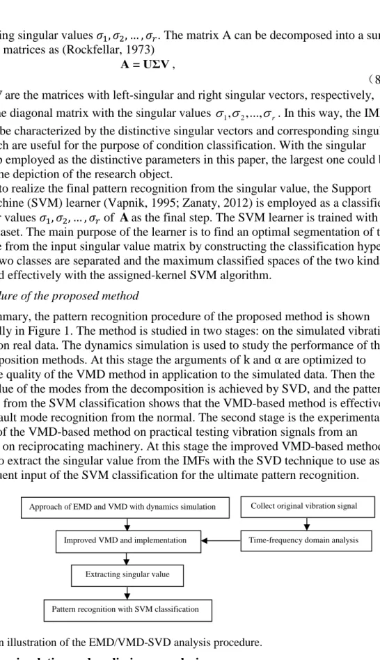
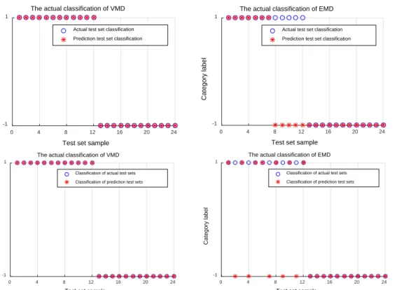
According to the algorithm requirement of the SVM classifier (Zanaty EA, 2012), 32 sets of the singular value samples extracted from the VMD decomposition of the two statuses were used as the input. Randomly selected 8 sets of feature vector were training data, the remaining 24 groups were test data. With the training completed, the normal signal samples were regarded as +1, and the samples of the fault signal as -1. 24 groups of samples were input into the fault classifier and the result is shown in Figure 7. The classification success rate with this method was 100%. While as the comparison with the proposed VMD based method, the fault identification rate of EMD was 79.2% with the same set of the input singular values.

Figure 7. Fault identification result (left is VMD, right is EMD).

4. Experimental validation

0 4 8 12 16 20 24

Test set sample -1

1

Category label

The actual classification of VMD

Actual test set classification Prediction test set classification

0 4 8 12 16 20 24

Test set sample -1

1

Category label

The actual classification of EMD

Actual test set classification Prediction test set classification

0 4 8 12 16 20 24

Test set sample

-1 1

Category label

The actual classification of VMD

Classification of actual test sets Classification of prediction test sets

0 4 8 12 16 20 24

Test set sample

-1 1

Category label

The actual classification of EMD

Classification of actual test sets Classification of prediction test sets

4.1. Experiment set-up

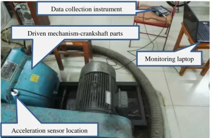
The experimental platform was composed of three parts: the reciprocating pump (type: BW250) with the driven mechanism of crankshaft components as the research target; the data collection system (IOtech640U) with an ICP accelerometer (sensitivity of 102 mV/g); and a monitoring and analysis system shown in Figure 8. The accelerometer was attached to the side of the driven mechanism (crankshaft parts). The sampling frequency was 10 kHz and the number of sampling points in each of the recorded time sequence was 1600. This number of points was found to be sufficient to capture representative sets of data at sufficient frequency resolution of 3.125 Hz in the frequency range of 0 – 5 kHz.

Figure 8. Experimental setup.

Aiming at the typical fault mode research, the driven mechanism that illustrated in the first picture in Figure 9 was taken apart and three types of the main faults were

introduced: (I) gear abrasion; (II) bearing bush scratched on the inner contact surface; and (III) end bearing with a ball peeled off.

Acceleration sensor location

Driven mechanism-crankshaft parts Data collection instrument

Figure 9. Faults setting in the crankshaft components.

4.2. Data acquisition and preliminary analysis

In order to avoid the coupling impact of water on the system in our experiment, the pump rotated with no load at the speed of 200 rev/min. The obtained vibration signal was obtained for normal, fault I, fault II and fault III conditions. Figure 10 presents the time histories of example signals recorded in the absence (a) and presence (b-d) faults. The results shown in Figure 10 suggest that the three typical faults cause a higher overall vibration magnitude, whereas Fault I and Fault II results in a distinct impacting vibration character. Figure 11 presents the spectrograms which correspond to the signals shown in Figure 10. The root mean square (RMS) magnitude of the spectra shows is clearly different in these four cases.

On account of typical failure mode of various mechanical components, the vibration magnitude of the fault modes increased in time domain description compared with the normal condition, nevertheless, they still share some generalities, e.g. the spectrum distribution of the four conditions in low-frequency stage are roughly similar, and their magnitudes in waterfall description are at the identical scale.

a. Normal b. Fault I

c. Fault II d. Fault III

Figure 10. Example time histories of the vibration signal recorded in the absence (a) and

presence (b-d) of the faults.

a.Normal b. Fault I 0 0.1 0.2 0.3 0.4 0.5 0.6 0.7 0.8 0.9 1 Time (s) -3 -2 -1 0 1 2 3 Amplitude (g) 0 0.1 0.2 0.3 0.4 0.5 0.6 0.7 0.8 0.9 1 Time (s) -6 -4 -2 0 2 4 6 Amplitude (g) 0 0.1 0.2 0.3 0.4 0.5 0.6 0.7 0.8 0.9 1 Time (s) -5 -4 -3 -2 -1 0 1 2 3 4 5 Amplitude (g) 0 0.1 0.2 0.3 0.4 0.5 0.6 0.7 0.8 0.9 1 Time (s) -4 -3 -2 -1 0 1 2 3 4 Amplitude (g)

c. Fault II d. Fault III

Figure 11. Waterfall plot of the vibration signal.

As to the fault modes, the impact feature is somehow illustrated by the energy clusters in the spectrum. The VMD-based method is employed to furtherly explore the

overshadowed difference of the time-frequency distribution among the normal and fault modes.

4.3. Model implementation

In order to find the number of IMF (k), the central frequency series, ω_k, of the modes are obtained through Hilbert transform, which is shown in Table 2. As previously mentioned, the value of k can be defined once two neighboring central frequencies are unveiled as close that may cause overlapping or over decomposition. As shown in Table 2 on this principle, The central frequency of the 6th IMF is nearly identical with the 7th as for the normal mode, therefore the decomposition terminates in the 6th step. In a similar fashion, the values of k of Fault I, II and III modes are sought as 6, 5, 5 so as to avoid frequency overlap in the decomposition process according to the former study. It also can be observed that the first three central frequencies of the four modes are similar with each other, while distinctive for high-order IMFs. This indicates that both the generality and distinctive impact feature involved in various frequency bands could be extracted with VMD method, so that it could be used as the mode comparison and recognition.

The decomposition results are shown in Figure 12 individually. We can find that most of the IMFs of each status through the improved VMD unveils the aperiodic feature of various conditions. To avoid mode overlap or even duplication, which is similar with the simulation study in the previous section, the balancing parameter of the data-fidelity constraint in the VMD was also set as 1000. Each of the characteristic vector of the decomposition modes was characterized by singular value from the SVD method, which may be set as the input of the classifier.

Table 2

Central frequency of the IMFs for different k.

Status IMF Central frequency /Hz

1 2 3 4 5 6 7

Normal 152 330 520 823 1190 1560 1570

Fault II 135 305 515 685 795 808

Fault III 155 294 478 653 865 870

a. Normal b. Fault I

c. Fault II d. Fault III

Figure 12. Signal decomposition.

0 0.2 0.4 0.6 0.8 1 -1 0 1 0 0.2 0.4 0.6 0.8 1 -1 0 1 0 0.2 0.4 0.6 0.8 1 -1 0 1 0 0.2 0.4 0.6 0.8 1 -1 0 1 0 0.2 0.4 0.6 0.8 1 -1 0 1 0 0.2 0.4 0.6 0.8 1 Time -1 0 1 Amplitude of IMFs 0 0.2 0.4 0.6 0.8 1 -1 0 1 0 0.2 0.4 0.6 0.8 1 -1 0 1 0 0.2 0.4 0.6 0.8 1 -1 0 1 0 0.2 0.4 0.6 0.8 1 -1 0 1 0 0.2 0.4 0.6 0.8 1 -1 0 1 0 0.2 0.4 0.6 0.8 1 Time -1 0 1 Amplitude of IMFs 0 0.2 0.4 0.6 0.8 1 -1 0 1 0 0.2 0.4 0.6 0.8 1 -1 0 1 0 0.2 0.4 0.6 0.8 1 -1 0 1 0 0.2 0.4 0.6 0.8 1 -1 0 1 0 0.2 0.4 0.6 0.8 1 Time -1 0 1 Amplitude of IMFs 0 0.2 0.4 0.6 0.8 1 -1 0 1 0 0.2 0.4 0.6 0.8 1 -1 0 1 0 0.2 0.4 0.6 0.8 1 -1 0 1 0 0.2 0.4 0.6 0.8 1 -1 0 1 0 0.2 0.4 0.6 0.8 1 Time -1 0 1 Amplitude of IMFs

In Table 3, the singular value of the normal and fault condition is obviously different with the impact feature in each state as the modal overlap avoided. The 24 groups of samples of normal, fault I, fault II and fault III were extracted from the VMD

decomposition and tested respectively. We randomly selected 8 groups of feature vector for classification training. The remaining 16 groups were tested data. When training samples classifier, the normal samples was selected as +1, the fault I as +2, fault II as +3, while fault III as +4.

Table 3

Singular values for the four conditions obtained with the VMD method.

Status k = 1 k = 2 k = 3 k = 4 k = 5 k = 6

Normal 5.6534 5.2394 4.7241 6.1244 3.6092 3.7025

Fault I 10.5952 10.2861 6.0257 6.2329 3.9251 3.8665

Fault II 12.3346 6.7968 5.5243 5.0209 4.0225

Fault III 16.2279 11.1894 9.5624 5.1258 3.9227

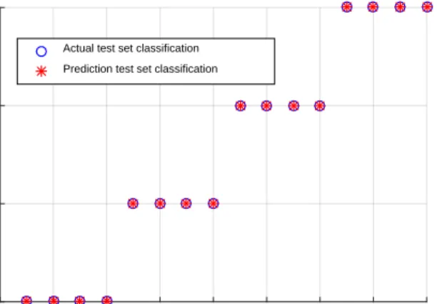
Figure 13. Faults identification.

Similar with the process of the simulation study, samples of 24 groups are set as the input of the multi-fault classifier here, through which the training is processed in the observation test as shown in Figure 13, the samples are identified by the SVM multi fault classifier recognition rate. The classification success rate for this method was 98%.

5. Conclusions

In order to accurately capture the impacting feature and identify the fault patterns of the driven mechanism of reciprocating machinery, an improved simulation and analysis method based on the VMD has been proposed. The method is based on acceleration data recorded on vibrating case of reciprocating machinery. The condition classification was carried out using the singular value decomposition applied to the IMFs matrix to obtain the vector with singular values. The obtained singular values were used to develop a train a suitable support vector machine. Simulated data were used to show that the improved VMD is superior to the EMD. It is shown that the method is 98% efficient when applied to real data recorded on reciprocating machinery with different faults. This work

illustrates that the method can overcome the deflect of mode overlap which tends to

0 2 4 6 8 10 12 14 16

Test set sample 1

2 3 4

Category label

The actual classification result

Actual test set classification Prediction test set classification

confuse popular pattern recognition algorithms. The research provides a new effective way for the reciprocating machinery fault diagnosis.

Declaration of Conflicting Interests

The author(s) declared no potential conflicts of interest with respect to the research, authorship, and/or publication of this article.

Funding

This research is supported by national Natural Science Foundation of China (Grant number 51175051) and Project of Jiangsu Overseas Research & Training Program for University Prominent Young & Middle-aged Teachers and Presidents.

References

Yang BS, Hwang WW, Kim DJ, et al (2010) Condition classification of small reciprocating compressor for refrigerators using artificial neural networks and support vector machines. Mechanical Systems and

Signal Processing, 19(2):371-390.

Bolaers F, Cousinard O, Estocp P, et al. (2011) Comparison of denoising methods for the early detection of fatigue bearing defects by vibratory analysis. Journal of Vibration and Control 17: 1983-1993. Kostyukov VN, Naumenko AP (2016) About the experience in operation of reciprocating compressors

under control of the vibration monitoring system. Procedia Engineering 152:497-504.

Ghamry MH, Reuben R.L., Steel JA (2010) The development of automated pattern recognition and statistical feature isolation techniques for the diagnosis of reciprocating machinery faults using acoustic emission. Mechanical Systems and Signal Processing 17(4):805-823.

Wang YF, Xue C, Jia XH, et al (2015) Fault diagnosis of reciprocating compressor valve with the method integrating acoustic emission signal and simulated valve motion. Mechanical Systems and Signal

Processing 56-57:1197-212.

Cui HX, Zhang LB, Kang RY et al (2009) Research on fault diagnosis for reciprocating compressor valve using information entropy and SVM method. Journal of Loss Prevention in the Process Industries 22(6):864-867.

Auger F, Flandrin P (1995) Improving the readability of time–frequency and time-scale representations by the reassignment method. Signal Process 43(5): 1068–1089

Jurado F, Saenz JR (2002) Comparison between discrete STFT and wavelets for the analysis of power quality events. Electronics Power System. Res. 62(3): 183–190.

Ghofrani S, McLernon DC (2009) Auto-Wigner–Ville distribution via non-adaptive and adaptive signal decomposition. Signal processing 89(8):1540-1549.

Loughlin PJ, Davidson KL (2001) Modified Cohen–Lee time–frequency distributions and instantaneous bandwidth of multicomponent signals. Signal Processing 49(6): 1153–1165

Baccigalupi A, Liccardo A (2016) The Huang Hilbert Transform for evaluating the instantaneous frequency evolution of transient signals in non-linear systems. Measurement 86: 1–13

Huang NE, Shen Z, Long SR, Wu MC, and et al. (1998) The empirical mode decomposition and the hilbert spectrum for nonlinear and non-stationary time series analysis, Proceedings of the Royal Society of

London A: Mathematical, Physical and Engineering Sciences 454: 903–995.

Zhang JW, Jiang Q, Ma B (2017) Signal de-noising method for vibration signal of flood discharge structure based on combined wavelet and EMD. Journal of Vibration and Control 23(15):2401-2417.

Dragomiretskiy K, Zosso D (2014) Variational mode decomposition. IEEE Transactions on Signal

Processing 62: 531–544.

Yue YJ, Sun G, Wang X (2016) Time-frequency analysis of ICE vibration base on VMD-PWVD. Journal of Wuhan University of Science and Technology 39(5): 365-370.

McNeill SI(2016) Decomposing a signal into short-time narrow-banded modes. Journal of Sound and

Vibration 373: 325–339.

Jiang.XX, Shunming Li, and Cheng C (2016) A Novel Method for Adaptive Multiresonance Bands Detection Based on VMD and Using MTEO to Enhance Rolling Element Bearing Fault Diagnosis.

Mohanty, Karunesh K.G., and Kota S.R. (2014) Bearing Fault Analysis Using Variational Mode Decompositon. 9th _{International Conference on Industrail and Information Systems}

(ICIIS).Rockafellar RT (1973) A dual approach to solving nonlinear programming problems by

unconstrained optimization. Mathematical Programming 5(1): 354–373.

Vapnik VN (1995) The Nature of Statistical Learning Theory. Springer New York, NY, USA. Zanaty EA (2012) Support Vector Machines (SVMs) versus Multilayer Perception (MLP) in data

classification. Egyptian Informatics Journal 13(3):177–183

Ranjbarkohan M., Rasekh M., Hoseini A.H., and et al. (2011) Kinematics and kinetic analysis of the slider-crank mechanism in onto linear four cylinder Z24 engine. Journal of Mechanical Engineering

Research 3(3): 85-95

Jomartov AA, Joldasbekov SU, and Drakunov Y. M. (2015) Dynamic synthesis of machine with slider-crank mechanism. Mechanical science 6: 35–40