Profiling relational data: a survey

DOI 10.1007/s00778-015-0389-y R E G U L A R PA P E R

Profiling relational data: a survey

Ziawasch Abedjan1 · Lukasz Golab2 · Felix Naumann3

Received: 1 August 2014 / Revised: 5 May 2015 / Accepted: 13 May 2015 / Published online: 2 June 2015 © Springer-Verlag Berlin Heidelberg 2015

Abstract Profiling data to determine metadata about a given dataset is an important and frequent activity of any IT professional and researcher and is necessary for vari-ous use-cases. It encompasses a vast array of methods to examine datasets and produce metadata. Among the simpler results are statistics, such as the number of null values and distinct values in a column, its data type, or the most frequent patterns of its data values. Metadata that are more difficult to compute involve multiple columns, namely correlations, unique column combinations, functional dependencies, and inclusion dependencies. Further techniques detect condi-tional properties of the dataset at hand. This survey provides a classification of data profiling tasks and comprehensively reviews the state of the art for each class. In addition, we review data profiling tools and systems from research and industry. We conclude with an outlook on the future of data profiling beyond traditional profiling tasks and beyond rela-tional databases.

B

1 _{MIT CSAIL, Cambridge, MA, USA} 2 _{University of Waterloo, Waterloo, Canada} 3 _{Hasso Plattner Institute, Potsdam, Germany}

1 Data profiling: finding metadata

Data profiling is the set of activities and processes to deter-mine the metadata about a given dataset. Profiling data is an important and frequent activity of any IT professional and researcher. We can safely assume that any reader of this article has engaged in the activity of data profiling, at least by eye-balling spreadsheets, database tables, XML files, etc. Possibly, more advanced techniques were used, such as key-word searching in datasets, writing structured queries, or even using dedicated data profiling tools.

Johnson gives the following definition: “Data profiling refers to the activity of creating small but informative sum-maries of a database” [79]. Data profiling encompasses a vast array of methods to examine datasets and produce metadata. Among the simpler results are statistics, such as the number of null values and distinct values in a column, its data type, or the most frequent patterns of its data values. Metadata that are more difficult to compute involve multiple columns, such as inclusion dependencies or functional dependencies. Also of practical interest are approximate versions of these dependencies, in particular because they are typically more efficient to compute. In this survey we preclude these and concentrate on exact methods.

Like many data management tasks, data profiling faces three challenges:(i)managing the input,(ii)performing the computation, and(iii)managing the output. Apart from typ-ical data formatting issues, the first challenge addresses the problem of specifying the expected outcome, i.e., determin-ing which profildetermin-ing tasks to execute on which parts of the data. In fact, many tools require a precise specification of what to inspect. Other approaches are more open and perform a wider range of tasks, discovering all metadata automatically.

The second challenge is the main focus of this survey and that of most research in the area of data profiling: The

com-putational complexity of data profiling algorithms depends on the number or rows, with a sort being a typical opera-tion, but also on the number of columns. Many tasks need to inspect all column combinations, i.e., they are exponen-tial in the number of columns. In addition, the scalability of data profiling methods is important, as the ever-growing data volumes demand disk-based and distributed processing.

The third challenge is arguably the most difficult, namely meaningfully interpreting the data profiling results. Obvi-ously, any discovered metadata refer only to the given data instance and cannot be used to derive schematic/semantic properties with certainty, such as value domains, primary keys, or foreign key relationships. Thus, profiling results need interpretation, which is usually performed by database and domain experts.

Tools and algorithms have tackled these challenges in different ways. First, many rely on the capabilities of the underlying DBMS, as many profiling tasks can be expressed as SQL queries. Second, many have developed innovative ways to handle the individual challenges, for instance using indexing schemes, parallel processing, and reusing interme-diate results. Third, several methods have been proposed that deliver only approximate results for various profiling tasks, for instance by profiling samples. Finally, users may be asked to narrow down the discovery process to certain columns or tables. For instance, there are tools that verify inclusion dependencies on user-suggested pairs of columns, but cannot automatically check inclusion between all pairs of columns or column sets.

Systematic data profiling, i.e., profiling beyond the occa-sional exploratory SQL query or spreadsheet browsing, is usually performed with dedicated tools or components, such as IBM’s Information Analyzer, Microsoft’s SQL Server Integration Services (SSIS), or Informatica’s Data Explorer.1 These approaches follow the same general procedure: A user specifies the data to be profiled and selects the types of metadata to be generated. Next, the tool computes the metadata in batch mode, using SQL queries and/or spe-cialized algorithms. Depending on the volume of the data and the selected profiling results, this step can last minutes to hours. Results are usually displayed in a vast collec-tion of tabs, tables, charts, and other visualizacollec-tions to be explored by the user. Typically, discoveries can then be translated to constraints or rules that are then enforced in a subsequent cleansing/integration phase. For instance, after discovering that the most frequent pattern for phone numbers is(ddd)ddd-dddd, this pattern can be promoted to arule stating that all phone numbers must be formatted accord-ingly. Most data cleansing tools can then either transform differently formatted numbers or mark them as improper.

1_{See Sect.6for a more comprehensive list of tools.}

We focus our discussion on relational data, the predomi-nant format of traditional data profiling methods, but we do cover data profiling for other data models in Sect.7.2. 1.1 Use-cases for data profiling

Data profiling has many traditional use-cases, including the data exploration, data cleansing, and data integration scenar-ios. Statistics about data are also useful in query optimization. Finally we describe several domain-specific use-cases, such as scientific data management and big data analytics. Data exploration Database administrators, researchers, and developers are often confronted with new datasets, about which they know nothing. Examples include data files down-loaded from the Web, old database dumps, or newly gained access to some DBMS. In many cases, such data have no known schema, no or old documentation, etc. Even if a for-mal schema is specified, it might be incomplete, for instance specifying only the primary keys but no foreign keys. A nat-ural first step is to understand how the data are structured, what they are about, and how much of them there are.

Such manual data exploration, or data gazing2, can and should be supported with data profiling techniques. Simple, ad hoc SQL queries can reveal some insight, such as the number of distinct values, but more sophisticated methods are needed to efficiently and systematically discover meta-data. Furthermore, we cannot always expect an SQL expert as the explorer, but rather “data enthusiasts” without formal computer science training [68]. Thus, automated data profil-ing is needed to provide a basis for further analysis. Morton et al. [107] recognize that a key challenge is overcoming the current assumption of data exploration tools that data are “clean and in a well-structured relational format.” Often data cannot be analyzed and visualized as is.

Database management A basic form of data profiling is the analysis of individual columns in a given table. Typically, the generated metadata include various counts, such as the num-ber of values, the numnum-ber of unique values, and the numnum-ber of non-null values. These metadata are often part of the basic statistics gathered by a DBMS. An optimizer uses them to estimate the selectivity of operators and perform other opti-mization steps. Mannino et al. [99] give a survey of statistics collection and its relationship to database optimization. More advanced techniques use histograms of value distributions, functional dependencies, and unique column combinations to optimize range queries [118] or for dynamic reoptimiza-tion [80].

2 _{“Data gazing involves looking at the data and trying to reconstruct} a story behind these data. […] Data gazing mostly uses deduction and common sense.” [104]

Database reverse engineering Given a “bare” database instance, the task of schema and database reverse engineer-ing is to identify its relations and attributes, as well as domain semantics, such as foreign keys and cardinalities [103,116]. Hainaut et al. [66] call these metadata “implicit constructs,” i.e., those that are not explicitly specified by DDL statements. However, possible sources for reverse engineering are DDL statements, data instances, data dictionaries, etc. The result of reverse engineering might be an entity-relationship model or a logical schema to assist experts in maintaining, integrating, and querying the database.

Data integration Often, the datasets to be integrated are unfamiliar and the integration expert wants to explore the datasets first: How large are they? What data types are needed? What are the semantics of columns and tables? Are there dependencies between tables and among databases?, etc. The vast abundance of (linked)open dataand the desire and potential to integrate them with local data has amplified this need.

A concrete use-case for data profiling is that ofschema matching, i.e., finding semantically correct correspondences between elements of two schemata [44]. Many schema matching systems perform data profiling to create attribute features, such as data type, average value length, and pat-terns, to compare feature vectors and align those attributes with the best matching ones [98,109].

Scientific data management and integration have cre-ated additional motivation for efficient and effective data profiling: When importing raw data, e.g., from scientific experiments or extracted from the Web, into a DBMS, it is often necessary and useful to profile the data and then devise an adequate schema. In many cases, scientific data are pro-duced by non-database experts and without the intention to enable integration. Thus, they often come with no adequate schematic information, such as data types, keys, or foreign keys.

Apart from exploring individual sources, data profiling can also reveal how and how well two datasets can be inte-grated. For instance, inclusion dependencies across tables from different sources suggest which tables might reasonably be combined with a join operation. Additionally, specialized data profiling techniques can reveal how much two relations overlap in their intent and extent. We discuss these challenges in Sect.7.1.

Data quality / data cleansing The need to profile a new or unfamiliar set of data arises in many situations, in general to prepare for some subsequent task. A typical use-case is pro-filing data to prepare adata cleansingprocess. Commercial data profiling tools are usually bundled with corresponding data quality / data cleansing software.

Profiling as a data quality assessment tool reveals data errors, such as inconsistent formatting within a column, miss-ing values, or outliers. Profilmiss-ing results can also be used to measure and monitor the general quality of a dataset, for instance by determining the number of records that do not conform to previously established constraints [81,117]. Gen-erated constraints and dependencies also allow for rule-based data imputation.

Big data analytics “Big data,” with its high volume, high velocity, and high variety [90], are data that cannot be man-aged with traditional techniques. Thus, data profiling gains a new importance. Fetching, storing, querying, and integrating big data are expensive, despite many modern technologies: Before exposing an infrastructure to Twitter’s firehose, it might be worthwhile to know about properties of the data one is receiving; before downloading significant parts of the linked data cloud, some prior sense of the integration effort is needed; before augmenting a warehouse with text min-ing results an understandmin-ing of its data quality is required. In this context, leading researchers have noted “If we just have a bunch of datasets in a repository, it is unlikely anyone will ever be able to find, let alone reuse, any of these data. With adequate metadata, there is some hope, but even so, challenges will remain[…] [7].”

Many big data and related data science scenarios call for data mining and machine learning techniques to explore and mine data. Again, data profiling is an important preparatory task to determine which data to mine, how to import it into the various tools, and how to interpret the results [120]. Further use-cases Knowledge about data types, keys, for-eign keys, and other constraints supports data modeling and helps keep data consistent, improves query optimization, and reaps all the other benefits of structured data management. Others have mentioned query formulation and indexing [126] and scientific discovery [75] as further motivation for data profiling. Also, compression techniques internally perform basic data profiling to optimize the compression ratio. Finally, the areas of data governance and data life-cycle management are becoming more and more relevant to busi-nesses trying to adhere to regulations and code. Especially concerned are financial institutions and health care organiza-tions. Again, data profiling can help ascertain which actions to take on which data.

1.2 Article overview and contributions

Data profiling is an important and practical topic that is closely connected to several other data management areas. It is also a timely topic and is becoming increasingly important given the recent trends in data science and big data analyt-ics [108]. While it may not yet be a mainstream term in the

database community, there already exists a large body of work that directly and indirectly addresses various aspects of data profiling. The goal of this survey is to classify and describe this body of work and illustrate its relevance to data-base research and practice. We also show that data profiling is far from a “done deal” and identify several promising direc-tions for future work in this area.

The remainder of this paper is organized as follows. In Sect. 2, we outline and define data profiling based on a new taxonomy of profiling tasks. Sections3,4, and5 sur-vey the state of the art of the three main research areas in data profiling: analysis of individual columns, analysis of multiple columns, and detection of dependencies between columns, respectively. Section6surveys data profiling tools from research and industry. We provide an outlook of data profiling challenges in Sect.7and conclude this survey in Sect.8.

2 Profiling tasks

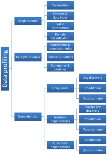
This section presents a classification of data profiling tasks. Figure 1 shows our classification, which includes single-column tasks, multi-single-column tasks and dependency detection. While dependency detection falls under multi-column pro-filing, we chose to assign a separate profiling class to this large, complex, and important set of tasks. The classes are discussed in the following subsections. We also highlight additional dimensions of data profiling, such as the type of storage, the approximation of profiling results, as well as the relationship between data profiling and data mining.

Collectively, a set of results of these tasks is called the data profileor database profile. In general, we assume the dataset itself as our only input, i.e., we cannot rely on query logs, schema, documentation.

2.1 Single-column profiling

A basic form of data profiling is the analysis of individual columns in a given table. Typically, the generated metadata comprise various counts, such as the number of values, the number of unique values, and the number of non-null values. These metadata are often part of the basic statistics gath-ered by the DBMS. In addition, the maximum and minimum values are discovered and the data type is derived (usu-ally restricted to string versus numeric versus date). More advanced techniques create histograms of value distributions and identify typical patterns in the data values in the form of regular expressions [122]. Data profiling tools display such results and can suggest actions, such as declaring a column with only unique values to be a key candidate or suggesting to enforce the most frequent patterns. As another exemplary

Da

ta

pr

ofiling

Summaries & sketches Dependencies Uniqueness Key discovery Condional (Approximate) Inclusion dependencies Foreign key discovery Condional (Approximate) Funconal dependencies Condional (Approximate)

Fig. 1 A classification of traditional data profiling tasks

use-case, query optimizers in database management systems also make heavy use of such statistics to estimate the cost of an execution plan.

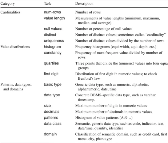
Table1lists the possible and typical metadata as a result of single-column data profiling. Some tasks are self-evident while others deserve more explanation. In Sect.3, we elabo-rate on the more interesting tasks, their implementation, and their use.

2.2 Multi-column profiling

The second class of profiling tasks covers multiple columns simultaneously. Multi-column profiling generalizes profil-ing tasks on sprofil-ingle columns to multiple columns and also identifies intervalue dependencies and column similarities. One task is to identify correlations between values through frequent patterns or association rules. Furthermore, cluster-ing approaches that consume values of multiple columns as features allow for the discovery of coherent subsets of data records and outliers. Similarly, generating summaries and sketches of large datasets relates to profiling values across columns.

Table 1 Overview of selected single-column profiling tasks (see Sect.3for details)

Category Task Description

Cardinalities num-rows Number of rows

value length Measurements of value lengths (minimum, maximum, median, and average)

null values Number or percentage of null values

distinct Number of distinct values; sometimes called “cardinality” uniqueness Number of distinct values divided by the number of rows Value distributions histogram Frequency histograms (equi-width, equi-depth, etc.)

constancy Frequency of most frequent value divided by number of rows

quartiles Three points that divide the (numeric) values into four equal groups

first digit Distribution of first digit in numeric values; to check Benford’s law

Patterns, data types, and domains

basic type Generic data type, such as numeric, alphabetic, alphanumeric, date, time

data type Concrete DBMS-specific data type, such as varchar, timestamp.

size Maximum number of digits in numeric values decimals Maximum number of decimals in numeric values patterns Histogram of value patterns (Aa9…)

data class Semantic, generic data type, such as code, indicator, text, date/time, quantity, identifier

domain Classification of semantic domain, such as credit card, first name, city, phenotype

Such metadata are useful in many applications, such as data exploration and analytics. Outlier detection is used in data cleansing applications, where outliers may indicate incorrect data values.

Section4 describes these tasks and techniques in more detail. It comprises multi-column profiling tasks that gen-erate metadata on horizontal partitions of the data, such as values and records, instead vertical partitions, such as columns and column groups. Although the discovery of col-umn dependencies, such as key or functional dependency discovery, also relates to multi-column profiling, we dedi-cate a separate section to dependency discovery as described next.

2.3 Dependencies

Dependencies are metadata that describe relationships among columns. The difficulties of automatically detecting such dependencies in a given dataset are twofold: First, pairs of columns or larger column sets must be examined, and second, the chance existence of a dependency in the data at hand does not imply that this dependency is meaningful. While much research has been invested in addressing the first challenge and is the focus of this survey, there is less work on seman-tically interpreting the profiling results.

A common goal of data profiling is to identify suitable keys for a given table. Thus, the discovery ofunique column combinations, i.e., sets of columns whose values uniquely identify rows, is an important data profiling task [70]. Once unique column combinations have been discovered, a second step is to identify among them the intended primary key of a relation.

A frequent real-world use-case of multi-column profiling is the discovery of foreign keys [96,123] with the help of inclusion dependencies [14,100]. An inclusion dependency states that all values or value combinations from one set of columns also appear in the other set of columns—a prereq-uisite for a foreign key.

Another form of dependency that is also relevant for data quality is the functional dependency (Fd). A func-tional dependency states that values in one set of columns functionally determine the value of another column. Again, much research has been performed to automatically detect

Fds [75,139]. Section5surveys dependency discovery

algo-rithms in detail.

Dependencies have many applications: An obvious use-case for functional dependencies is schema normalization. Inclusion dependencies can suggest how to join two relations, possibly across data sources. Their conditional counterparts help explore the data by focusing on certain parts of the dataset.

2.4 Conditional, partial, and approximate solutions Real datasets usually contain exceptions to rules. To account for this, dependencies and other constraints detected by data profiling can be relaxed. We describe two relaxations below: partial and approximate.

Partial dependencieshold for only a subset of the records, for instance, for 95 % of the records or for all but 10 records. Such dependencies are especially valuable in data cleansing scenarios: They are patterns that hold for almost all records and thus should probably hold forallrecords if the data were clean. Violating records can be extracted and cleansed [129]. Once a partial dependency has been detected, it is inter-esting to characterize for which records it holds, i.e., if we can find a condition that selects precisely those records. Conditional dependenciescan specify such conditions. For instance, a conditional unique column combination might state that the columnstreetis unique for all records withcity = ‘NY.’ Conditional inclusion dependencies (Cinds) were proposed by Bravo et al. for data cleaning and contextual schema matching [19]. Conditional functional dependencies (Cfds) were introduced in [46], also for data cleaning.

Approximate dependencies and other constraints are unconditional statements, but are not guaranteed to hold for the entire relation. Such dependencies are often discovered using sampling [76] or other summarization techniques [31]. Their approximate nature is often sufficient for certain tasks, and approximate dependencies can be used as input to the more rigorous task of detecting true dependencies. This sur-vey does not discuss such approximation techniques.

2.5 Types of storage

Data profiling tasks are applicable to a wide range of sit-uations in which data are provided in various forms. For instance, most commercial profiling tools assume that data reside in a relational database, make use of SQL queries and indexes. In other situations, for instance, a csv file is provided and a data profiling method needs to create its own data struc-tures in memory or on disk. And finally, there are situations in which a mixed approach is useful: Data that were originally in the database are read once and processed further outside the database.

The discussion and distinction of such different situa-tions is relevant when evaluating the performance of data profiling algorithms and tools. Can we assume that data are already loaded into main memory? Can we assume the pres-ence of indices? Are profiling results, which can be quite voluminous, written to disk? Fair comparisons need to estab-lish a level playing field with same assumptions about data storage.

2.6 Data profiling versus data mining

A clear, well-defined, and accepted distinction between data profiling and data mining does not exist. Two criteria are conceivable:

1. Distinction by the object of analysis: instance versus schema or columns versus rows

2. Distinction by the goal of the task: description of existing data versus new insights beyond existing data.

Following the first criterion, Rahm and Do distinguish data profiling from data mining by the number of columns that are examined: “Data profiling focuses on the instance analysis of individual attributes. […] Data mining helps discover spe-cific data patterns in large datasets, e.g., relationships holding between several attributes” [121]. While this distinction is well defined, we believe several tasks, such as Ind or Fd

detection, belong to data profiling, even if they discover rela-tionships between multiple columns.

We believe a different distinction along both criteria is more useful: Data profiling gathers technical metadata to support data management; data mining and data analytics discovers non-obvious results to support business manage-ment with new insights. While data profiling focuses mainly on columns, some data mining tasks, such as rule discovery or clustering, may also be used for identifying interesting characteristics of a dataset. Others, such as recommendation or classification, are not related to data profiling.

With this distinction, we concentrate on data profiling and put aside the broad area of data mining, which has already received unifying treatment in numerous textbooks and surveys. However, in Sect. 4, we address the subset of unsupervised mining approaches that can be applied on unknown data to generate metadata and hence serves the pur-pose of data profiling.

Classifications of data mining tasks include an overview by Chen et al., who distinguish the kinds of databases (rela-tional, OO, temporal, etc.), the kinds of knowledge to be mined (association rules, clustering, deviation analysis, etc.), and the kinds of techniques to be used [130]. We make a sim-ilar distinction in this survey. In particular, we distinguish the different classes of data profiling tasks and then exam-ine various techniques to perform them. We discuss profiling non-relational data in Sect.7.

2.7 Summary

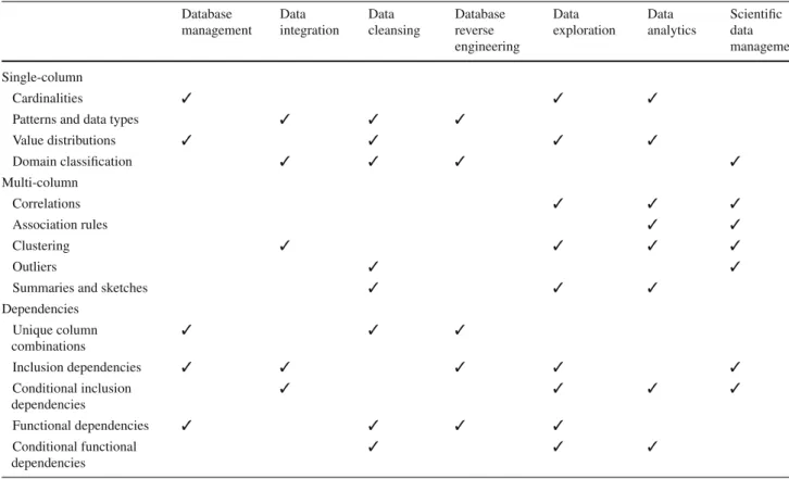
We summarize this section by connecting the various data profiling tasks with the use-cases mentioned in the introduc-tion. Conceivably, any task can be useful for any use-case, depending on the context, the properties of the data at hand,

Table 2 Data profiling tasks and their primary use-cases Database management Data integration Data cleansing Database reverse engineering Data exploration Data analytics Scientific data management Single-column Cardinalities ✓ ✓ ✓

Patterns and data types ✓ ✓ ✓

Value distributions ✓ ✓ ✓ ✓ Domain classification ✓ ✓ ✓ ✓ Multi-column Correlations ✓ ✓ ✓ Association rules ✓ ✓ Clustering ✓ ✓ ✓ ✓ Outliers ✓ ✓

Summaries and sketches ✓ ✓ ✓

Dependencies Unique column combinations ✓ ✓ ✓ Inclusion dependencies ✓ ✓ ✓ ✓ ✓ Conditional inclusion dependencies ✓ ✓ ✓ ✓ Functional dependencies ✓ ✓ ✓ ✓ Conditional functional dependencies ✓ ✓ ✓

etc. Table2lists the profiling tasks and their primary use-cases.

3 Column analysis

The analysis of the values of individual columns is usually a straightforward task. Table1lists the typical metadata that can determined for a given column. The following sections describe each category of tasks in more detail, mention-ing possible uses of the respective results. In [104], a book addressing practitioners, several of these tasks are discussed in more detail.

3.1 Cardinalities

Cardinalities or counts of values in a column are the most basic form of metadata. The number of rows in a table (num-rows) reflects how many entities (e.g.,customers,orders, items) are represented in the data, and it is relevant to data management systems, for instance to estimate query costs or to assign storage space.

Information about the length of values in terms of char-acters (value length), including the length of the longest and shortest value and the average length, is useful for schema reverse engineering (e.g., to determine tight data type

bounds), outlier detection (e.g., single-character first names), and formatting (dates have the same min-, max- and average length).

The number of empty cells, i.e., cells with null values or empty strings (null values), indicates the (in-)completeness of a column. The number of distinct values (distinct) allows query optimizers to estimate selectivity of selection or join operations: The more distinct values there are, the more selec-tive such operations are. To users, this number can indicate a candidate key by comparing it with the number of rows. Alternatively, this number simply illustrates how many dif-ferent values are present (e.g., how many customers have ordered something or how many cities appear in an address table).

Determining the number of rows, metadata about value lengths, and the number of null values is straightforward and can be performed in a single pass over the data. Determining the number ofdistinct valuesis more involved: Either hashing or sorting all values is necessary. When hashing, the number of non-empty buckets must be counted, taking into account hash collisions, which further add to the count. When sorting, a pass through the sorted data counts the number of values, where groups of same values are counted only once.

From the number of distinct values theuniquenesscan be calculated, which is typically defined as the number of unique values divided by the number of rows. Note that the number

of distinct values can also be estimated using the minHash technique discussed in Sect.4.3.

Apart from determining the exact number of distinct val-ues, query optimization is a strong incentive toestimatethose counts in order to predict query execution plan costs with-out actually reading the entire data. Because approximate profiling is not the focus of this survey, we give only two exemplary pointers. Haas et al. [65] base their estimation on data samples and describe and empirically compare various estimators from the literature. Other works do scan the entire data but use only a small amount of memory to hash the values and estimate the number of distinct values, an early example being [11].

3.2 Value distribution

Value distributions are more fine-grained cardinalities, namely the cardinalities of groups of values. Histograms are among the most common profiling results. A histogram stores frequencies of values within well-defined groups, usu-ally by dividing the ordered set of values into a fixed set of buckets. The buckets of equi-width histograms span value ranges of same length, while the buckets of equi-depth (or equi-height) histograms each represent the same number of value occurrences. A common special case of an equi-depth histogram is dividing the data into fourquartiles. A more general concept isbiased histograms, which can adapt their accuracy for different regions[33]. Histograms are used for database optimization as a rough probability distribution to avoid a uniform distribution assumption and thus provide better cardinality estimations [77]. In addition, histograms are interpretable by humans, as their visual representation is easy to comprehend.

Theconstancyof a column is defined as the ratio of the frequency of the most frequent value (possibly a pre-defined default value) and the overall number of values. It thus rep-resents the proportion of some constant value compared with the entire column.

A particularly interesting distribution is the first digit dis-tribution for numeric values. Benford’s law [15] states that in naturally occurring numbers the distribution of the first digit dof a number approximately followsP(d)=log10(1+_d1). Thus, the 1 is expected to be the most frequent leading digit, followed by 2, etc. Benford and others have observed this behavior in many sets of numbers, such as molecular weights, building sizes, and electricity bills. In fact, the law has been used to uncover accounting fraud and other fraudulently cre-ated numbers.

Determining the above distributions usually involves a sin-gle pass over the column, except for equi-depth histograms (i.e., with fixed bucket sizes) and quartiles, which determine bucket boundaries through sorting. In the same manner or

through hashing the most frequent value can be discovered to determine constancy.

Finally, many more things can be counted and aggregated in a column. For instance, some profiling tools and meth-ods determine among others the frequency distribution of soundex code, n-grams, and others, the inverse frequency dis-tribution, i.e., the distribution of the frequency disdis-tribution, or the entropy of the frequency distribution of the values in a column [82].

3.3 Types and patterns

The profiling tasks of this section are ordered by increasing semantic richness (see also Table1). We start with the most simple observable properties, move on to specific patterns of the values of a column, and end with the semantic domain of a column.

Discovering thebasic typeof a column, i.e., classifying it as numeric, alphabetic, alphanumeric, date, or time, is fairly simple: The presence or absence of numeric and non-numeric characters already distinguishes the first three. The latter two can usually be recognized by the presence of numbers only within certain ranges, and by numbers separated in regu-lar patterns by special symbols. Recognizing the actual data type, for instance among the SQL types, is similarly easy. In fact, data of many data types, such astimestamp,boolean, or int, must follow a fixed, sometimes DBMS-specific pat-tern. When classifying columns into data types, one should choose the most specific data type—in particular avoiding the catchallscharorvarcharif possible. For the data types decimal,float, anddouble, one can additionally extract the maximum number of digits and decimals to determine the metadatasizeanddecimals.

A common and useful data profiling result is the extrac-tion of frequent patterns observed in the data of a col-umn. Then, data that do not conform to such a pattern are likely erroneous or ill-formed. For instance, a pat-tern for phone numbers might be informally encoded as +dd (ddd) ddd ddddor as a simple regular expression

\(\d3\)\ − \d3\ − \d4).3A challenge when determining

frequent patterns is to find a good balance between generality and specificity. The regular expression.*is the most general and matches any string. On the other hand, the expression data allows only that one single string. For the Potter’s Wheel tool, Raman and Hellerstein [122] suggest finding the data pattern with the minimal description length (MDL). They model description length as a combination of precision, recall, and conciseness and provide an algorithm to enumer-ate all possible patterns. The RelIE system was designed 3 _{A more detailed regular expression, taking into account different} for-matting options and different restrictions (e.g., phone numbers cannot begin with a 1), can easily reach 200 characters in length.

for information extraction from textual data [92]. It creates regular expressions based on training data with positive and negative examples by systematically, greedily transforming regular expressions. Finally, Fernau [51] provides a good characterization of the problem of learning regular expres-sions from data and presents a learning algorithm for the task. This work is also a good starting point for further reading

The semanticdomainof a column describes not the syntax of its values but their meaning. While a regular expression might characterize a column, labeling it as “phone number” provides a concrete domain. Clearly, this task cannot be fully automated, but some work has been done for common-place domains about persons, places, etc. Zhang et al. take a first step by clustering columns that have the same meaning across the tables of a database [144], which they extend to the par-ticularly difficult area of numeric values in [142]. In [133] the authors take the additional step of matching columns to pre-defined semantics from the person domain. Knowledge of the domain is not only of general data profiling interest, but also of particular interest to schema matching, i.e., the task of finding semantic correspondences between elements of different database schemata.

3.4 Data completeness

Explicitmissing data are simple to characterize: For each col-umn, we report the number of tuples with a null or a default value. However, datasets may containdisguisedmissing val-ues. For example, Web forms often include fields whose values must be chosen from pull-down lists. The first value from the pull-down list may be pre-populated on the form, and some users may not replace it with a proper or correct value due to lack of time or privacy concerns. Specific exam-ples include entering 99999 as the zip code of an address or leaving “Alabama” as the pre-populated state (in the US, Alabama is alphabetically the first state). Of course, for some records, Alabama may be the true state.

Detecting disguised default values is difficult. One heuris-tic solution is to examine each column at a time, and, for each possible value, compute the distribution of the other attribute values [74]. For example, if Alabama is indeed a disguised default value, we expect a large subset of tuples withstate= Alabama(i.e., those whose true state is different) to form an unbiased sample of the whole relation.

Another instance in which profiling missing data is not trivial involves timestamped data, such as measurement or transaction data feeds. In some cases, tuples are expected to arrive regularly, e.g., in datacenter monitoring, every machine may be configured to report its CPU utilization every minute. However, measurements may be lost en route to the data-base, and overloaded or malfunctioning machines may not report any measurements at all. [60]. In contrast to detecting missing attribute values, here we are interested in

estimat-ing the number of missestimat-ing tuples. Thus, the profilestimat-ing task may be to single out the columns identified as being of type timestamp, and, for those that appear to be distributed uni-formly across a range, infer the expected frequency of the underlying data source and estimate the number of miss-ing tuples. Of course, sometimestampcolumns correspond to application timestamps with no expectation of regularity, rather than data arrival timestamps. For instance, in an online retailer database, order dates and delivery dates are generally not expected to be scattered uniformly over time.

4 Multi-column analysis

Profiling tasks over a single column can be generalized to projections of multiple columns. For example, there has been work on computing multi-dimensional histograms for query optimization [41,119]. Multi-column profiling also plays an important role in data cleansing, e.g., in assessing and explaining data glitches, which often occur in column com-binations [40].

In the remainder of this section, we discuss statistical methods and data mining approaches for generating meta-data based on co-occurrences and dependencies of values across attributes. We focus on correlation and rule mining approaches as well as unsupervised clustering and learning approaches; machine learning techniques that require train-ing data or detailed knowledge of the data are beyond the scope of data profiling.

4.1 Correlations and association rules

Correlation analysis reveals related numeric columns, e.g., in an Employees table,ageandsalarymay be correlated. A straightforward way to do this is to compute pairwise correla-tions among all pairs of columns. In addition to column-level correlations, value-level associations may provide useful data profiling information.

Traditionally, a common application of association rules has been to find items that tend to be purchased together based on point-of-sale transaction data. In these datasets, each row is a list of items purchased in a given transaction. An associa-tion rule {bread}→{butter}, for example, states that if a transaction includes bread, it is also likely to include butter, i.e., customers who buy bread also buy butter. A set of items is referred to as anitemset, and an association rule specifies an itemset on the left-hand side and another itemset on the right-hand side.

Algorithms for generating association rules from data decompose the problem into two steps [8]:

1. Discover all frequent itemsets, i.e., those whose fre-quencies in the dataset (i.e., theirsupport) exceed some

threshold. For instance, the itemset {bread,butter} may appear in 800 out of a total of 50,000 transactions for a support of 1.6 %.

2. For each frequent itemseta, generate association rules of the forml → a −l withl ⊂ a, whoseconfidence exceeds some threshold. Confidence is defined as the frequency ofa divided by the frequency ofl, i.e., the conditional probability oflgivena−l. For example, if the frequency of {bread,butter} is 800 and the fre-quency of {bread} alone is 1000, then the confidence of the association rule {bread}→ {butter} is 0.8. That is, if bread is purchased, there is an 80 % chance that butter is also purchased in the same transaction. In the context of relational data profiling, association rules denote relationships or patterns between attribute val-ues among columns. Consider an Employees table with fields name, employee number, department,position, and allowance. We may find a frequent itemset of the form {department=finance,position =assistant manager,allowance=$1000} and a corresponding asso-ciation rule of the form {department=finance,position = assistant manager} → {allowance = $1000}. This would be the case if most or all assistant managers in the finance department were assigned an allowance budget of $1000.

While the second step mentioned above is straightforward (generating association rules from frequent itemsets), the first step is computationally expensive due to the large number of possible frequent itemsets (or patterns of values) [72]. Pop-ular algorithms for efficiently discovering frequent patterns include Apriori [8], Eclat [141], and FP-Growth [67].

The Apriori algorithm exploits the observation that all subsets of a frequent itemset must also be frequent. In the first iteration, Apriori finds all frequent itemsets of size one, i.e., those containing one item or one attribute value. In the next iteration, only the frequent itemsets of size one are expanded to find frequent itemsets of size two, and so on.

There are also several optimized versions of Apriori, such as DHP [115] and RARM [35]. FP-Growth discov-ers frequent itemsets without a candidate generation step. It transforms the database into an extended prefix tree of frequent patterns (FP-tree). The FP-Growth algorithm tra-verses the tree and generates frequent itemsets by pattern growth in a depth-first manner. Finally, Eclat is based on intersecting transaction-id (TID) sets of associated itemsets and is best suited for dealing with large frequent itemsets. Eclat’s strategy for identifying frequent itemsets is similar to Apriori.

Negative correlation rules, i.e., those that identify attribute values thatdo notco-occur with other attribute values, may also be useful in data profiling to find anomalies and out-liers [21]. However, discovering negative association rules is

more difficult, becauseinfrequentitemsets cannot be pruned in the same way as frequent itemsets, and therefore, novel pruning rules are required [135].

Finally, we note that in addition to using existing tech-niques, such as correlations and association rules for pro-filing, extensions have been proposed, such as discovering linear dependencies between columns [25].

However, in this approach, the user has to choose the subset of attributes to be analyzed. We discuss dependency discovery in more detail in Sect.5.

4.2 Clustering and outlier detection

Another useful profiling task is to segment the records into homogeneous groups using a clustering algorithm; further-more, records that do not fit into any cluster may be flagged as outliers. Cluster analysis can identify groups of similar records in a table, while outliers may indicate data qual-ity problems. For example, Dasu and Johnson [36] cluster numeric columns and identify outliers in the data. Further-more, based on the assumption that data glitches occur across attributes and not in isolation [16], statistical inference has been applied to measure glitch recovery in [39].

Another example of clustering in the context of data profil-ing is ProLOD++, which appliesk-means clustering toRdf

relations [1]. We refer the reader to surveys by Jain et al. [78] and Xu and Wunsch II [137] for more details on clustering algorithms for relational data.

4.3 Summaries and sketches

Besides clustering, another way to describe data is to create summaries or sketches [23]. This can be done by sampling or hashing data values to a smaller domain. Sketches have been widely applied to answering approximate queries, data stream processing and estimating join sizes [37,54,111]. Cormode et al. [31] give an overview of sketching and sam-pling for approximate query processing.

Another interesting task is to assess the similarity of two columns, which can be done using multi-column hashing techniques. The Jaccard similarity of two columns A and B is |A ∩B|/|A∪ B|, i.e., the number of distinct values they have in common divided by the total number of distinct values appearing in them. This gives the relative number of values that appear in bothAandB. Since semantically similar values may have different formats, we can also compute the Jaccard similarity of the n-gram distributions inAandB. If the distinct value sets of columnsAandBare not available, we can estimate the Jaccard similarity using theirMinHash signatures[38].

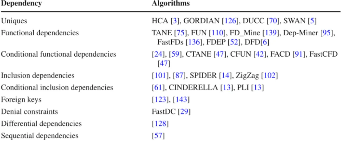
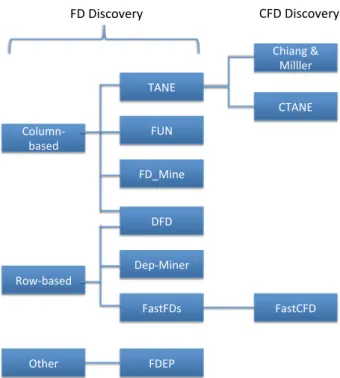
Table 3 Dependency discovery

algorithms Dependency Algorithms

Uniques HCA [3], GORDIAN [126], DUCC [70], SWAN [5] Functional dependencies TANE [75], FUN [110], FD_Mine [139], Dep-Miner [95],

FastFDs [136], FDEP [52], DFD[6]

Conditional functional dependencies [24], [59], CTANE [47], CFUN [42], FACD [91], FastCFD [47]

Inclusion dependencies [101], [87], SPIDER [14], ZigZag [102] Conditional inclusion dependencies [61], CINDERELLA [13], PLI [13]

Foreign keys [123], [143]

Denial constraints FastDC [29]

Differential dependencies [128] Sequential dependencies [57]

5 Dependency detection

We now survey various formalisms for detecting depen-dencies among columns and algorithms for mining them from data, including keys and unique column combinations (Sect. 5.1), functional dependencies (Sect. 5.2), inclusion dependencies (Sect.5.3), and other types of dependencies that are relevant to data profiling (Sect.5.4). Table3lists the algorithms that are discussed.

We use the following symbols:RandSdenote relational schemata, withrandsdenoting instances ofRandS, respec-tively. The number of columns inRis|R|and the number of tuples inr is|r|. We refer to tuples ofr andsasri andsj, respectively. Subsets of columns are denoted by uppercase X,Y,Z(with|X|denoting the number of columns inX) and individual columns by uppercaseA,B,C. Furthermore, we defineπX(r)andπA(r)as the projection ofron the attribute setX or attributeA, respectively; thus,|πX(r)|denotes the count of district combinations of the values ofX appearing inr. Accordingly,ri[A]indicates the value of the attributeA of tupleriandri[X] =πX(ri). We refer to an attribute value of a tuple as acell.

The number of potential dependencies inrcan be expo-nential in the number of attributes|R|; see Fig. 2 for an illustration of all possible subsets of the attributes in Table4. This means that any dependency discovery algorithm has a worst-case exponential time complexity. There are two classes of heuristics that have appeared in the literature.

Fig. 2 Powerset lattice for the example Table4

Table 4 Example dataset

Tuple id First Last Age Phone

1 Max Payne 32 1234

2 Eve Smith 24 5432

3 Eve Payne 24 3333

4 Max Payne 24 3333

Column-based or top-down approaches start with “small” dependencies (in terms of the number of attributes they ref-erence) and work their way to larger dependencies, pruning candidates along the way whenever possible. Row-based or bottom-up approaches attempt to avoid repeated scanning of the entire relation during candidate generation. While these approaches cannot reduce the worst-case exponential complexity of dependency discovery, experimental studies have shown that column-based approaches work well on tables containing a very large number of rows and row-based approaches work well for wide tables [6,113]. For more details on the computational complexity of variousFdand

Inddiscovery algorithms, we refer the interested reader to [94].

5.1 Unique column combinations and keys

Given a relation R with instancer, a unique column com-bination (a “unique”) is a set of columns X ⊆ R whose projection onrcontains only unique value combinations. Definition 1 (Unique) A column combination X ⊆ Ris a unique, iff∀ri,rj ∈r,i = j : ri[X] =rj[X].

Analogously, a set of columns X ⊆ R is anon-unique column combination(a “non-unique”), iff its projection onr contains at least one duplicate value combination.

Definition 2 (Non-unique) A column combination X ⊆ R is anon-unique, iff∃ri,rj ∈r,i = j : ri[X] =rj[X].

Each superset of a unique is also unique while each subset of a non-unique is also a non-unique. Therefore, discovering all uniques and non-uniques can be reduced to the discovery of minimal uniques and maximal non-uniques:

Definition 3 (Minimal Unique) A column combinationX ⊆ Ris aminimal unique, iff∀X⊂X :Xis a non-unique. Definition 4 (Maximal Non-Unique) A column combina-tion X ⊆ R is amaximal non-unique, iff∀X ⊃ X : X is a unique.

Aprimary keyis a unique that was explicitly chosen to be the unique record identifier while designing the table schema. Since the discovered uniqueness constraints are only valid for a relational instance at a specific point of time, we refer to uniques and non-uniques instead of keys and non-keys. A further distinction can be made in terms of possible keys and certain keys when dealing with uncertain data and NULL values [86].

The problem of discovering a minimal unique of size k≤nis NP-complete [97]. To discover all minimal uniques and maximal non-uniques of a relational instance, in the worst case, one has to visit all subsets of the given relation, no matter the strategy (breadth-first or depth-first) or direction (bottom-up or top-down). Thus, the discovery of all minimal uniques and maximal non-uniques of a relational instance is an NP-hard problem and even the solution set can be expo-nential [64].

Given|R|, there can be||RR|| 2

≥2|R2|_{minimal uniques in the}

worst case, as all combinations of size|R₂|can simultaneously be minimal uniques.

5.1.1Gordian: row-based discovery

Row-based algorithms require multiple runs over all column combinations as more and more rows are considered. They benefit from the intuition that non-uniques can be detected without considering every row. A recursive unique discovery algorithm that works this way isGordian[126]. The algo-rithm consists of three parts:(i)Pre-organize the data in form of a prefix tree,(ii)find maximal non-uniques by traversing the prefix tree,(iii)compute minimal uniques from maximal non-uniques.

The prefix tree is stored in main memory. Each level of the tree represents one column of the table, whereas each branch stands for one distinct tuple. Tuples that have the same values in their prefix share the corresponding branches. For example, all tuples that have the same value in the first column share the same node cells. The time to create the prefix tree depends on the number of rows; therefore, this can be a bottleneck for very large datasets.

The traversal of the tree is based on the cube operator [63], which computes aggregate functions on projected columns.

Non-unique discovery is performed by a depth-first traver-sal of the tree for discovering maximum repeated branches, which constitute maximal non-uniques.

After discovering all maximal non-uniques, Gordian

computes all minimal uniques by generating minimal com-binations that are not covered by any of the maximal non-uniques. In [126] it is stated that this complementation step needs only quadratic time in the number of minimal uniques, but the presented algorithm implies cubic runtime: For each non-unique, the updated set of minimal uniques must be simplified by removing redundant uniques. This simplification requires quadratic runtime in the number of uniques. As the number of minimal uniques is bound lin-early by the numbersof maximal non-uniques, the runtime of the unique generation step isO(s3).

Gordian exploits the intuition that non-uniques can be discovered faster than uniques. Non-unique discovery can be aborted as soon as one repeated value is discovered among the projections. The prefix structure of the data facilitates this analysis. It is stated that the algorithm is polynomial in the number of tuples for data with a Zipfian distribution of values. Nevertheless, in the worst case, Gordian has exponential runtime.

The generation of minimal uniques from maximal non-uniques can be a bottleneck if there are many maximal non-uniques. Experiments showed that in most cases the unique generation dominates the runtime [3]. Furthermore, the approach is limited by the available main memory. Although data may be compressed because of the prefix structure of the tree, the amount of processed data may still be too large to fit in main memory.

5.1.2 Column-based traversal of the column lattice

The problem of finding minimal uniques is comparable to the problem of finding frequent itemsets [8]. The well-known Apriori approach is applicable to minimal unique discovery, working bottom-up as well as top-down. With regard to the powerset lattice of a relational schema, the Apriori algorithms generate all relevant column combinations of a certain size and verify those at once. Figure2illustrates the powerset lat-tice for the running example in Table4. The effectiveness and theoretical background of those algorithms is discussed by Giannela and Wyss [55]. They presented three breadth-first traversal strategies: a bottom-up, a top-down, and a hybrid traversal strategy.

Bottom-up unique discovery traverses the powerset lat-tice of the schema R from the bottom, beginning with all 1-combinations toward the top of the lattice, which is the

|R|-combination. The prefixed numberk ofk-combination indicates the size of the combination. The same notation applies fork-candidates,k-uniques, andk-non-uniques. To generate the set of 2-candidates, we generate all pairs of

1-non-uniques.k-candidates withk > 2 are generated by extending the(k−1)-non-uniquesby another non-unique column. After the candidate generation, each candidate is checked for uniqueness. If it is identified as a non-unique, thek-candidateis added to the list ofk-non-uniques.

If the candidate is verified as unique, its minimality has to be checked. The algorithm terminates when k =

|1-non-uniques|. A disadvantage of this candidate generation technique is that redundant uniques and duplicate candidates are generated and tested.

The Apriori idea can also be applied to the top-down approach. Having the set of identifiedk-uniques, one has to verify whether the uniques are minimal. Therefore, for eachk-unique, all possible(k−1)-subsetshave to be gener-ated and verified. The hybrid approach generates thekth and

(n−k)th levels simultaneously. Experiments have shown that in most datasets, uniques usually occur in the lower levels of the lattice, which favors bottom-up traversal [3].

Hca is an improved version of the bottom-up Apriori technique [3].Hcaoptimizes the candidate generation step, applies statistical pruning and considers functional depen-dencies that have been inferred on the fly. In terms of candidate generation,Hca applies the optimized join that was introduced for frequent itemset mining [8].Hca

gener-ates candidgener-ates by combining only(k−1)-non-uniquesthat share the firstk−2 elements. If no such two non-uniques exist, no candidates are generated and the algorithm termi-nates before reaching the last level of the powerset lattice. Further pruning can be achieved by considering value his-tograms and distinct counts that can be retrieved on the fly in previous levels. For example, consider the1-non-uniqueslast andagefrom Table4. The column combination {last,age} cannot be a unique based on the value distributions. While the value “Payne” occurs three times inlast, the column agecontains only two distinct values. That means at least two of the rows containing the value “Payne” also have a duplicate value in theagecolumn. Using the count distinct values,Hcadetects functional dependencies on the fly and leverages them to avoid unnecessary uniqueness checks.

WhileHcaimproves existing bottom-up approaches, it

does not perform the early identification of non-uniques in a row-based manner done byGordian. Thus,Gordian is faster on datasets with many non-uniques, but Hcaworks

better on datasets with many minimal uniques. 5.1.3 DUCC: traversing the lattice via random walk While the breadth-first approach for discovering minimal uniques gives the most pruning, a depth-first approach might work well if there are relatively few minimal uniques that are scattered on different levels of the powerset lattice. Depth-first detection of unique column combinations resembles the problem of identifying the most promising paths through the

lattice to discover existing minimal uniques and avoid unnec-essary uniqueness checks.Duccis a depth-first approach that

traverses the lattice back and forth based on the uniqueness of combinations [70]. Following a random walk principle by randomly adding columns to non-uniques and removing columns from uniques,Ducctraverses the lattice in a manner that resembles the border between uniques and non-uniques in the powerset lattice of the schema.

Ducc starts with a seed set of2-non-uniquesand picks a seed at random. Eachk-combination is checked using the superset/subset relations and pruned if any of them subsumes the current combination. If no previously identified combi-nation subsumes the current combicombi-nation Ducc performs uniqueness verification. Depending on the verification,Ducc

proceeds with an unchecked(k−1)-subset or(k−1)-superset of the current k-combination. If no seeds are available, it checks whether the set of discovered minimal uniques and maximal non-uniques correctly complement each other. If so,Duccterminates; otherwise, a new seed set is generated by complementation.

Duccalso optimizes the verification of minimal uniques

by using a position list index (PLI) representation of val-ues of a column combination. In this index, each position list contains the tuple ids that correspond to the same value combination. Position lists with only one tuple id can be dis-carded, so that the position list index of a unique contains no position lists. To obtain the PLI of a column combination, the position lists in PLIs of all contained columns have to be cross-intersected. In fact,Duccintersects two PLIs in a similar way in which a hash join operator would join two relations. As a result of using PLIs,Ducc can also apply row-based pruning, because the total number of positions decreases with the size of column combinations. Intuitively, combining columns makes the contained combination values more specific and therefore more likely to be distinct.

Ducc has been experimentally compared to Hca, a

column-based approach, andGordian, a row-based unique

discovery algorithm. SinceDucccombines row-based and column-based pruning, it performs significantly better [70]. Experiments on smaller datasets showed that while Hca

outperformsGordianon low-dimensional data with many uniques,GordianoutperformsHcaon datasets with many attributes but few uniques [3].

Furthermore the random walk strategy allows a distributed application ofDuccfor better scalability.

5.1.4 SWAN: an incremental approach

Swanmaintains a set of indexes to efficiently find the new sets of minimal uniques and maximal non-uniques after inserting or deleting tuples [5].Swanbuilds such indexes based on existing minimal uniques and maximal non-uniques in a way that avoids a full table scan.Swanconsists of two

main components: theInserts Handlerand theDeletes Han-dler. The Inserts Handler takes as input a set of inserted tuples, checks all minimal uniques for uniqueness, finds the new sets of minimal uniques and maximal non-uniques, and updates the repository of minimal uniques and maximal non-uniques accordingly. Similarly, the Deletes Handler takes as input a set of deleted tuples, searches for duplicates in all maximal non-uniques, finds the new sets of minimal uniques and maximal non-uniques, and updates the repository accord-ingly.

5.2 Functional dependencies

Afunctional dependency(Fd) overRis an expression of the formX → A, indicating that∀ri,rj ∈r ifri[X] =rj[X]; then,ri[A] =rj[A]. That is, any two tuples that agree on Xmust also agree on A. We refer toXas the left-hand side (LHS) andAas the right-hand side (RHS). Givenr, we are interested in finding all non-trivial and minimalFdsX → A that hold onr, with non-trivial meaning A∩ X = ∅ and minimal meaning that there must not be anyFdY → Afor

anyY ⊂X. A naive solution to theFddiscovery problem is as follows.

For each possible RHS A

For each possible LHSX ∈ R\A For each pair of tuplesri andrj

Ifri[X] =rj[X]andri[A] =rj[A]Break ReturnX → A

This algorithm is prohibitively expensive: For each of the

|R| possibilities for the RHS, it tests 2(|R|−1) possibilities for the LHS, each time having to scanr multiple times to compare all pairs of tuples. However, notice that forX → A to hold, the number of distinct values ofXmust be the same as the number of distinct values ofX A—otherwise at least one combination of values ofXthat is associated with more than one value ofA, thereby breaking theFd[75]. Thus, if we

pre-compute the number of distinct values of each combination of one or more columns, the algorithm simplifies to:

For each possible RHS A

For each possible LHSX ∈ R\A

If|πX(r)| = |πX A(r)|

ReturnX→ A

Recall Table4. We have|πphone(r)| = |πage,phone(r)| =

|πlast,phone(r)|. Thus, phone → age and phone →

lasthold. Furthermore,|πlast,age(r)| = |πlast,age,phone(r)|,

implying {last,age}→phone.

The above algorithm is still inefficient due to the need to compute distinct value counts and test all possible col-umn combinations. As was the case with unique discovery,

Fddiscovery algorithms employ row-based (bottom-up) and

Fig. 3 Classification of algorithms for functional dependency discov-ery and their extensions to conditional functional dependencies

column-based (top-down) optimizations, as discussed below. Figure3lists the algorithms that are discussed, along with their extensions to conditionalFddiscovery, which are cov-ered in Sect.5.2.4. An extensive experimental evaluation of variousFddiscovery algorithms on different datasets,

scal-ing in both the number of rows and the number of columns, is presented in [113].

5.2.1 Column-based algorithms

As was the case with uniques, Apriori-like approaches can help prune the space ofFds that need to be examined, thereby optimizing the first two lines of the above straightforward algorithms. TANE [75], FUN [110], and FD_Mine [139] are three algorithms that follow this strategy, with FUN and FD_Mine introducing additional pruning rules beyond TANE’s based on the properties ofFds. They start with sets

of single columns in the LHS and work their way up the powerset lattice in a level-wise manner. Since only min-imal Fds need to be returned, it is not necessary to test

possibleFds whose LHS is a superset of an already found

Fdwith the same RHS. For instance, in Table4, once we find that phone → ageholds, we do not need to consider

{first,phone} →age,{last,phone} →age, etc.

Additional pruning rules may be formulated from Arm-strong’s axioms, i.e., we can prune from consideration those

Fds that are logically implied by those we have found so far. For instance, if we find that A → B andB → A, then we can prune all LHS column sets includingB, because A

andB are equivalent [139]. Another pruning strategy is to ignore columns sets that have the same number of distinct values as their subsets [110]. Returning to Table4, observe that phone → first does not hold. Since |πphone(r)| =

|πlast,phone(r)| = |πage,phone(r)| = |πlast,age,phone(r)|, we

know that addinglastand/orageto the LHS cannot lead to a validFdwithfirston the RHS. To determine these cardinal-ities the approaches use a so-called partition data structure, which is similar to the PLIs of Sect.5.1.3.

5.2.2 Row-based algorithms

Row-based algorithms examine pairs of tuples to determine LHS candidates. Dep-Miner [95] and FastFDs [136] are two examples; the FDEP algorithm [52] is also row-based, but the way it ultimately findsFds that hold is different.

The idea behind row-based algorithms is to compute the so-called difference sets for each pair of tuples, which are the columns on which the two tuples differ. Table5 enu-merates the difference sets in the data from Table4. Next, we can find candidate LHS’s from the difference sets as fol-lows. Pick a candidate RHS, say,phone. The difference sets that include phone, with phoneremoved are as follows: {first,last,age}, {first,age}, {age}, {last} and {first,last}. This means that there exist pairs of tuples with different val-ues of phoneand also with different values of these five difference sets. Next, we find minimal subsets of columns that have a non-empty intersection with each of these differ-ence sets. Such subsets are exactly the LHS’s of minimalFds with phone as the RHS: If two tuples have different values ofphone, they are guaranteed to have different values of the columns in the above minimal subsets, and therefore, they do not causeFdviolations. Here, there is only one such min-imal subset, {last,age}, giving {last,age}→phone. If we repeat this process for each possible RHS, and compute min-imal subsets corresponding to the LHS’s, we obtain the set of minimalFds. The main difference among row-basedFd

discovery algorithms is in how they find the minimal subsets. A recent approach toFddiscovery is DFD, which adapts the column-based and row-based pruning of the unique dis-covery approachDuccto the problem ofFddiscovery [6].

Table 5 Difference sets computed from Table4

Tuple ID pair Difference set

(1,2) first, last, age, phone

(1,3) first, age, phone

(1,4) age, phone

(2,3) last, phone

(2,4) first, last, phone

(3,4) first

DFD decomposes the attribute lattice into|R|lattices, con-sidering each attribute as a possible RHS of anFd. For the

remaining|R| −1 attributes, DFD applies a random walk approach by pruning supersets of FdLHS’s and subsets of non-FdLHS’s.

DFD has been experimentally compared to TANE, which is a column-based approach, and FastFDs, which is row-based [6]. The experiments confirm that row-based approa-ches work well on high-dimensional tables with a relatively small number of tuples, while column-based approaches, such as TANE, perform better on low-dimensional tables with a large number of rows. DFD, which benefits from row-based and column-based pruning, performs significantly better than TANE and FastFDs, unless the table has very many tuples and very few columns or vice versa.

5.2.3 Partial and approximate functional dependencies WhileFds were meant for schema design and were enforced by the database management system, there are many instan-ces in which a database may not satisfy someFds exactly. For

example, the application semantics may have changed over time andFdenforcement was disabled, or the database may have been created by integrating conflicting data sources. As a result, it is useful to discoverpartialorsoftFds, i.e., those

which “almost hold,” perhaps with a few exceptions. A common definition of “almost holding” or “confidence” is the relative size of the largest subset ofron which a given

Fdholds exactly divided by|r|[58,85]. For example, if we remove tuple 1 from Table4, theFdlast → phoneholds exactly, and therefore, its confidence is 3₄. The CORDS sys-tem for finding softFds uses a slightly different definition: The confidence ofX → Ais |πX(r)|

|πX A(r)| [76]. Other definitions

involve computing the number of tuples or tuple pairs that do not violate theFddivided by|r|or|r|2, respectively [85].

A related notion is that ofapproximateFdinference, in which partial or exact Fds are generated from a sample of

a relation [76,85]. Of course, even if an Fd holds exactly on a subset of a relation, it may hold partially on the whole relation. ApproximateFdinference is appealing from a

com-putational standpoint as it requires only a sample of the data. 5.2.4 Conditional functional dependencies

Conditional functional dependencies (Cfds), proposed in [46], encodeFds that hold only on well-defined subsets of r. For instance, {first,last} → age does not hold on the entire relation in Table4, but it does hold on a subset of it wherefirst = Eve. Formally, aCfdconsists of two parts: an embedded Fd X → A and an accompanying pattern

tuplewith attributes X A. Each cell of a pattern tuple con-tains a value from the corresponding attribute’s domain or a wildcard symbol “_”. A pattern tuple identifies a subset of a