Generating cutting planes through inequality merging on multiple variables in knapsack problems

(1)

GENERATING CUTTING PLANES THROUGH INEQUALITY

MERGING ON MULTIPLE VARIABLES IN KNAPSACK PROBLEMS

by

THOMAS CHARLES BOLTON

B.S., Kansas State University, 2015

A THESIS

Submitted in partial fulfillment of the requirements for the degree

MASTER OF SCIENCE

Department of Industrial and Manufacturing Systems Engineering College of Engineering

KANSAS STATE UNIVERSITY Manhattan, Kansas

2015

Approved by:

Major Professor Todd Easton

(2)

ABSTRACT

Integer programming is a field of mathematical optimization that has applications across a wide variety of industries and fields including business, government, health care and mili-tary. A commonly studied integer program is the knapsack problem, which has applications including project and portfolio selection, production planning, inventory problems, profit maximization applications and machine scheduling. Integer programs are computationally difficult and currently require exponential effort to solve.

Adding cutting planes is a way of reducing the solving time of integer programs. These cutting planes eliminate linear relaxation space. The theoretically strongest cutting planes are facet defining inequalities.

This thesis introduces a new class of cutting planes called multiple variable merging cover inequalities (MVMCI). The thesis presents the multiple variable merging cover algo-rithm (MVMCA), which runs in linear time and produces a valid MVMCI. Under certain conditions, an MVMCI can be shown to be a facet defining inequality. An example demon-strates these advancements and is used to prove that MVMCIs could not be identified by any existing techniques.

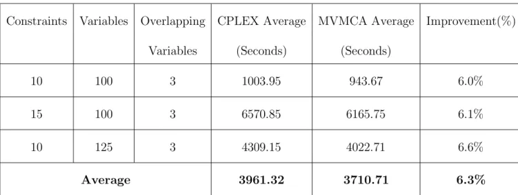
A small computational study compares the computational impact of including MVMCIs. The study shows that finding an MVMCI is extremely fast, less than .01 seconds. Further-more, including an MVMCI improved the solution time required by CPLEX, a commercial integer programming solver, by 6.3% on average.

(3)

List of Figures

(6)

List of Tables

2.1 Benefits and Weights of Items . . . 13

3.1 Calculating MVMCAα0 _{Results . . . .} ₃₁

3.2 Affinely Independent Points . . . 32

3.3 Reversed MVMCAα Results . . . 36

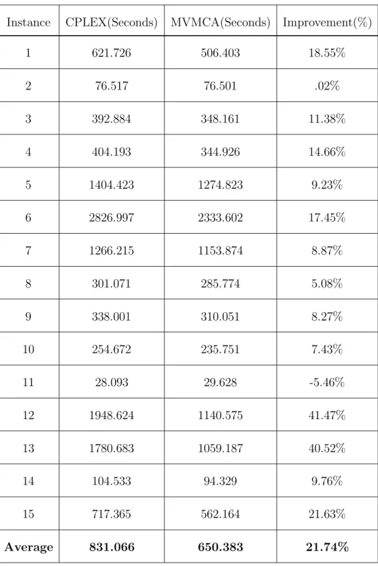
4.1 MVMCA Smaller Problem Runs . . . 41

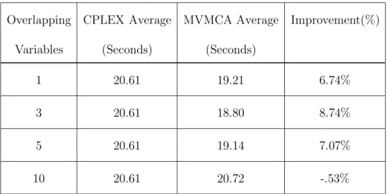
4.2 Overlapping Variables Averages . . . 42

4.3 MVMCA Larger Problem Runs . . . 43

(7)

Dedication

This work is dedicated to my parents, John and Susan, and siblings, Jen, Ben, Amanda and James, for their unconditional love and support.

(8)

Acknowledgments

I would first thank Dr. Todd Easton. Without his excellent mentorship, scholarly support and patience, this thesis would not have been possible.

I am also grateful to Dr. Jessica Heier Stamm and Dr. Bette Grauer for their participation on my Supervisory Committee.

Lastly, I want to sincerely thank the people of Kansas State University, especially the faculty, staff and students of the Industrial and Manufacturing Systems Engineering Department. My personal growth, educational development and professional endeavors have greatly benefitted from my relationships with these individuals.

(9)

Chapter 1 Introduction

Integer programming is a field of mathematical optimization with great potential to trans-form the world and improve people’s lives. Integer programming has applications in a wide variety of business, technical and personal situations where finding the optimal solution to a problem is the goal. It is easiest to explain the contributions of integer programming by looking at how it is applied in the world today.

One area where integer programs are widely used is in various types of vehicle routing problems. In Ankara, Turkey, there were problems stemming from the costs associated with busing students from rural regions to schools. Once the problem was formulated as an integer program, the researchers [3] were able to decrease the overall cost by 28% and reduce the total miles traveled by all buses by 14%. Other benefits obtained were an increased utilization of 27% and a decreased variation in capacity by 33%.

There are numerous other applications of integer programs (IPs). IPs have been used to assist with cancer location and treatment [33]. IPs has also been applied to the overseas

(10)

shipping industry [39] and facilities layout [16]. Other applications include military appli-cations [37], sports scheduling [14], airline security [35] and criminal justice assignment [6], which have all benefitted society.

While IPs are very useful, solving IP problems isN P hard, which means that there does not exist a polynomial time algorithm to solve the problem to optimality, unless P =N P. In laymans terms it means that any algorithm used to solve an IP requires exponential time. Thus, certain concessions are typically made to the IP model, which leave open the chance that the solution that is found is suboptimal in the real world. This means that the solution needs to be evaluated to make sure it is implementable and that it provides benefit to the process.

There are a few different ways to solve an IP. The most widely used algorithm is the branch and bound algorithm. Branch and bound [32] works by solving the linear relaxation and then branching on one of the non-integer variables. Branch and bound is a good strategy for smaller problems, but as the problems get larger, the time to solve these problems increases exponentially. While computers are constantly getting faster and more advanced, there still exist IPs that cannot be solved to optimality.

One common method to reduce the IP solution time is through cutting planes. Cutting planes help to decrease the solving time of integer programming software by decreasing the space of the linear relaxation that the software might check. It is called a cutting plane because it cuts off these undesirable noninteger solutions. Thus, many cutting plane preprocessing techniques are used to help reduce IP’s solution time.

(11)

called facet defining. If all facet defining inequalities are added to an IP, then its linear relaxation solution is integer. Thus, branch and bound only requires one iteration and not exponential effort.

This thesis focuses on a specific class of IPs called a knapsack problem. Knapsack prob-lems are found in various settings related to pricing of items [4], defense [1], aviation security [28] and portfolio selection [38].

A commonly used cutting plane for a knapsack problem are cover inequalities. Occasion-ally, a cover inequality can be facet defining, but most cover inequalities can be strengthened. Fundamentally, this thesis takes a cover inequality and strengthens it.

1.1 Research Motivation and Questions

In 2014, Hickman and Easton [24] generated inequalities by merging two cover inequalities together. This resulted in a new class of cutting planes for the knapsack instances. Further-more under certain conditions, these merged cover inequalities could be facet defining.

Hickman’s results could only merge covers on a single variable. That is, the covers had to have exactly one element in common. In certain instances, Hickman and Easton’s method would create inequalities that were weak and these inequalities could be strengthened.

The motivation for this thesis is to build on and stregthen their work. Thus, this work sought to answer the following reseasrch questions. Can cover inequalities be merged on mul-tiple variables? Can merging be done so that the inequalities created cannot be dominated by an inequality of the similar form?

(12)

1.2 Research Contributions

The primary contribution of this thesis is the development of a new class of cutting planes for the knapsack problem that decreases the time to solve integer programs. This class is called multiple variable merging cover inequalities (MVMCI). These inequalities merge two cover inequalities from an existing constraint on multiple variables. They are merged with the aid of a merging coefficient. This coefficient,α, is also the theoretically strongest coefficient that can be obtained. Furthermore, this class of cutting planes cannot be obtained by current methods without the consultation of an oracle.

An algorithm is also presented, which generates MVMCI from a single knapsack con-straint. This algorithm runs in linear time, which is the theoretically best run time possible. It also can generate facet defining inequalities, which are the theoretically strongest inequal-ities.

To show the usefulness of MVMCIs, a computational study was conducted. The multiple variable merging cover algorithm (MVMCA) was coded into C and added to CPLEX [10], a commercial integer program solver, for small and medium problems, and run to completion. The time required to solve these problems is referred to as run time. MVMCA has the ability to decrease run times of CPLEX solver by up to 40% in this computational study on certain instances. In addition, MVMCI was able to cut CPLEX run times by on average 6.3% on the medium sized problems, which reduced the run time by over an hour.

(13)

1.3 Outline

This thesis is organized as follows: Chapter 2 presents an overview of the background in-formation that is necessary to understand the contributions of this thesis. It covers integer programming, polyhedral theory, knapsack problems, cover cuts, and lifting examples. This includes formal definitions, explanations and examples to aid in the understanding of the background material.

Chapter 3 provides the theoretical basis for inequality merging on multiple variables. It contains the theorems, explanations and conditions for validity of the merged inequality. An example where multiple variable merging cover algorithm creates a facet defining inequality demonstrates these concepts. The run time is discussed and it is shown that it is not dom-inated by previous methods. Chapter three ends with an argument that these inequalities are new and not simply a rehashing of previous work.

Chapter 4 is a computational study to show the usefulness of MVMCI. The results are interpreted and it is shown that MVMCA can be easily implemented and the inequalities generated can be useful in solving knapsack integer programs.

Finally, Chapter 5 is a summary of the important contributions from this thesis. It also offers up possible areas of future research.

(14)

Chapter 2 Background Information

Chapter 2 gives an overview of the background information necessary to grasp the contribu-tions of this thesis. This includes an overview of integer programming as well as polyhedral theory. The use of cutting planes to shorten the process of solving an IP is also discussed along with lifting. Lastly an overview and example of Hickman’s inequality merging tech-nique is discussed.

2.1 Integer Programming

An integer program (IP) is a mathematical model of the form maximize cT_x _{subject to}

Ax≤b, x≥0 and x∈Zn _where_A_∈_Rmxn_{, b}_∈_Rm _and_c_∈_Rn_{. Define the set of feasible IP}

solutions as P ={x∈Zn

+ :Ax≤b} and the set of indices to be N ={1, ..., n}.

An important concept in solving IP’s is a linear relaxation (LR). Given an IP, its linear relaxation is the IP with the integer requirement removed, meaning that the problem is

(15)

a linear program of the form maximize cTx subject to Ax ≤ b, x ≥ 0. Define the linear relaxation space as PLR ₌ _{_x _∈ _R _: _Ax _≤ _{b, x} _≥ ₀_}_{. The optimal solution to a linear}

relaxation can be found in polynomial time [29].

Branch and bound is the most widely used and standard algorithm to solve integer programming optimization problems [32]. This technique builds an ancestral branching tree where the nodes have properties determined by the nodes’ lineage. This technique generates an optimal solution, but it may take an exponential amount of time.

The branch and bound algorithm starts with the linear relaxation, called the root node. If no noninteger variables exist, then the linear relaxation solution is optimal. If not, the node is split on a noninteger variable (xi =f) of the LR solution. The resulting branched

child nodes each have one constraint on them xi ≥ dfe and xi ≤ bfc, the integer below and

above the noninteger xi. While there exists at least one unfathomed leaf node, the branch

and bound algorithm solves the LR of that node with its corresponding linear relaxation solution, x∗LR and linear relaxation objective function value, z∗LR. This repeats until all nodes have been fathomed. A node is fathomed if one of three criteria are met: the linear relaxation becomes infeasible, the node’s linear relaxation solution is integer or the objective function value is worse than the best integer solution found so far.

To reduce the run time of branch and bound, cutting planes are frequently applied. The area of research that studies cutting planes is called polyhedral theory. The goal of a cutting plane is to shrink the linear relaxation space. The next section gives an overview of polyhedral theory.

(16)

2.2 Polyhedral Theory

The geometry of any IP problem is important to the solution of the IP. Polyhedral theory is fundamental to understanding this type of research. A half space is {x⊆Rn _:

n

P

i=1

αixi ≤β}

and a polyhedron is defined as the intersection of finitely many half spaces.

A set S ⊆Rn _{is convex if and only if} _λx1_{+ (1}₋_λ)x2 _∈_S _{for every}_λ _∈_[0,_{1] and all} _x1

and x2 ∈ S. The convex hull of a set S, conv(S), is the intersection of all convex sets that contain S. Clearly, a polyhedron is convex. An important result is that PLR _and _conv(P₎

are both polyhedrons. If a polyhedron is bounded, then it is called a polytope. An inequality

n

P

i=1

αixi ≤β is valid for conv(P) if everyx∈P satisfies this inequality. A

valid inequality is a cutting plane if there exists an x0 ∈ PLR such that

n

P

i=1

αix0i > β. Only

cutting planes can reduce the time required to solve an IP.

Every valid inequality induces a face, F, of conv(P) where F = {x ∈ conv(P) :

Pn

i=1αixi = β}. Every face is a polyhedron. Theoretically, the usefulness of a valid

in-equality is measured by the dimension of this face.

The dimension of a polyhedron equals the maximum number of linearly independent vectors. However, an IP only has feasible points and so no nonzero vector creates a feasi-ble direction. Due to this fact, affine independence is used to determine the dimension of conv(P).

Let V be a finite set of points in Rn_, _V ₌ _{_vi _∈ _Rn _: _i _{= 1, ..., w}_}_{. The points in} _V

are affinely independent if and only if the unique solution to

w P i=1 λivi = 0 and w P i=1 λi = 0 is

(17)

points is equal to the maximum number of affinely independent points minus one. In order to define points in Rn_{, let} _ξ

j be the origin in n dimensions translated one positive unit in

the jth dimension, i.e. ξ2 = (0,1,0, ...,0).

The larger the dimension of the face, up to one less than the dimension of conv(P), the theoretically stronger the inequality is. The strongest such cutting planes are called facet defining inequalities. An inequality is facet defining if its face has dimension one less than the dimension of conv(P). A facet defining inequality is an inequality that defines a facet of the conv(P). If one could find all of the facet defining inequalities for a given problem, then including all these facets would define conv(P). Thus, the extreme points would be integer and the linear relaxation solution would be an integer solution.

2.2.1 2-Dimensional Integer Programming Example

The following small example of a two dimensional IP is shown to explain these concepts.

Maximize x1+x2

Subject to: 5x1+ 4x2 ≤ 20

x1+ 2x2 ≤ 8

x1, x2 ≥ 0

x1, x2 ∈ Z

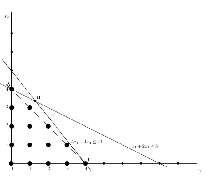
Figure 2.1 shows a graphical representation of this problem. The set of feasible integer points, P, are identified by large circles. The extreme points of the linear relaxation space are shown at A, B, C and the origin. The dashed line denotes the conv(P) and is formed by connecting the extreme integer points in the feasible region. Note thex axis from the origin

(18)

to (4,0) and theyaxis from the origin to (0,4) are also assumed to be dashed in this picture. y y y y y t t t t t 0 1 2 3 4 y y y y t t t 1 2 3 4 y y y y y y \ \ \ \ \ \ \ \ \ \ \ \ \ \ \ \ \ \ \ \ \ \ \ \ \ H H H H H H H H H H H H H H H H H H H H H H H H H H H H H H H H H H H HH @ @ @ @ @ @ @ @ @ A C B t x1+ 2x2≤8 5x1+ 4x2≤20 x1 x2

Figure 2.1: 2-Dimensional IP Example

The first step in solving this problem with cutting planes is to find the linear relaxation solution. Once that is found, a cutting plane is added to the linear relaxation and the linear relaxation solution is recalculated to be (x∗LR_{, z}∗LR_{). This process is repeated until the}

solution is an integer solution in which case z∗LR is the optimal integer objective function valuez∗I P.

(19)

Because the objective function is simplyx1+x2, the best solution to this problem occurs

at (1.3,3.375), which is point A, and yields z∗LR _{= 4.675. Adding the valid inequality,}

x1+x2 ≤4, to the formulation eliminates the point (1.3,3.375). Thus, this valid inequality

is a cutting plane. Resolving the linear relaxation results in an optimal solution ofz∗LR = 4 at the point (4,0). Since this is an integer point, the optimal IP solution is found.

To provex1+x2 ≤4 is a facet defining inequality, one must first determine the dimension

of conv(P). The dimension of conv(P) is 2 because it is bounded from the top by the fact that there are 2 variables and bounded from below by the fact that there are 3 affinely independent points inP : (0,0),(0,1) and (1,0). Combining these two statements means that the dimension of conv(P) is 2.

The constraintx1+x2 ≤4 is valid as it does not eliminate any points inP. Furthermore,

the face F ={x∈ conv(P) : x1+x2 = 4} is not conv(P) since (0,0) is in P and not inF.

Thus, the dimension of the face, dim(F), is less than or equal to 1. The points (0,4) and (2,2) are in P and also in F. These points are affinely independent. Thus, dim(F) ≥ 1. Thus x1+x2 ≤4 is a facet defining inequality.

Knapsack problems are used extensively in this thesis. Whence, the next section formally introduces knapsack problems and demonstrates them through the use of an example.

2.3 Knapsack Problems

Knapsack problems (KP) are a special class of IPs. The knapsack problem is so named by the concept problem where a hiker needs to select which items to bring on an overnight

(20)

camping trip and has limited strength. Each possible item has a corresponding non-negative weight and benefit. The purpose is to maximize the benefit the hiker receives from the items in his knapsack subject to constraints on how much weight the hiker can carry.

To model the knapsack as an IP, let xj = 1 if item j is taken and 0 else. Then the

KP is Maximize n P j=1 cjxj subject to n P j=1

ajxj ≤ b, and xj ∈ {0,1} for all j ∈ N where c and

a∈Rn

+, b∈R+. Denote the feasible solutions of a KP asPKP ={x∈ {0,1}n :

n

P

j=1

ajxj ≤b}.

The multiple knapsack problem (MK) is a type of integer program with a finite number of knapsack constraints. It is defined as Maximize cT_x _{subject to} _Ax _≤ _b _and _x _{∈ {}_0,₁_}n

wherec∈Rn+, A∈R

m∗n

+ . Define the feasible solutions of an MK to beP

M K

={x ∈ {0,1}n: Ax≤b}.

Both KP and MK problems have many real life applications that many researchers have worked on in a variety of fields and industries. These applications include project and portfolio selection [7], production planning and inventory problems [11], profit maximization applications [13, 36] and machine scheduling [30].

Without loss of generality, assume that any KP has the property that a1 ≥a2 ≥...≥an.

Furthermore, in the remainder of the document, assume that every subset of N is sorted in ascending order. Finally, assume a1 ≤b. If not, then x1 = 0 for all feasible solutions and x1

can be removed from the problem. Given these assumptions, dim(conv(PKP_{)) =}_n _because

the origin and ξi for all i ∈ N are in PKP. The conv(PM K) is full dimensional assuming

that eachaij ∈A satisfiesaij ≤bi, for all i= 1, ..., m and j = 1, ..., n.

To assist with understanding the concepts of knapsack problems an example is shown. This example contains the classic hiker with a knapsack. This example shows the setup and

(21)

solution to the KP problem.

A hiker considers taking 15 items on a fishing trip to Yellowstone National Park. He can take any of the items at his own discretion, subject to the constraints. Each item has a corresponding weight and benefit as shown in Table 2.1. Furthermore, the hiker can only carry 40 units.

Object 1 2 3 4 5 6 7 8 9 10 11 12 13 14 15

Weight 21 17 16 15 12 11 10 8 7 6 5 4 3 3 1

Benefit 30 30 16 15 1 18 14 11 10 7 9 12 7 2 4 Table 2.1: Benefits and Weights of Items

The hiker can choose to take an item in which case xj = 1, or not take the item in which

case xj = 0. The problem can be formulated as an integer programming model as shown.

Maximize: 30x1+ 30x2 + 16x3+ 15x4+ 1x5+ 18x6+ 14x7 + 11x8+ 10x9

+7x10+ 9x11+ 12x12+ 7x13+ 2x14+ 4x15

Subject to 21x1+ 17x2 + 16x3+ 15x4+ 12x5 + 11x6+ 10x7+ 8x8+ 7x9+ 6x10

+5x11+ 4x12+ 3x13+ 3x14+ 1x15 ≤40

xi ∈ {0,1} ∀i={1, ...,15}

Solving this shows that the maximum benefit the hiker can obtain is 76 by carrying items 2, 6, 11, 12 and 13. The hiker is carrying a total weight to carry of 40 units.

(22)

2.4 Cover Inequalities

One widely used technique for solving KP and MK problems is by adding a cover cut to the constraints of the problem. Given a knapsack constraint, a set C ⊆ N is a cover for a KP if P

j∈C

aj > b. The corresponding cover inequality takes the form

P

j∈C

xj ≤ |C| −1. This

inequality is valid because it is created from the original KP constraints and carrying every element in the cover is too heavy. Thus, the hiker can carry at most one item less than the number in the cover.

A coverC is a minimal cover ifC\ {j}is not a cover for allj ∈C. If C ⊆N is a cover, define an extended cover as E(C) =C∪ {j ∈N : aj ≥ai,∀i∈ C}. An extended cover has

a valid inequality of the form P

j∈E(C)

xj ≤ |C| −1.

Recall the example of the hiker in Yellowstone. A cover of the weight constraint, for example, would be {1,2,3} because 21 + 17 + 16 > 40 and the resulting cover constraint would be x1 +x2 +x3 ≤ 2. This is also a minimal cover because if any element is taken

out of the cover, it ceases to be a cover. An example of a non-minimal cover is {1,2,3,4}

because element 4 can be taken out of the cover and it remains a cover. Minimal covers are the most desirable covers. In fact, a nonminimal cover inequality is dominated by a minimal cover inequality.

In order to understand that the concepts in this thesis are new, it is important to un-derstand different types of lifting. Lifting is similar to multiple variable merging. Thus, to understand the difference between multiple variable merging and lifting, background infor-mation on lifting is covered next.

(23)

2.5 Lifting

Lifting is used to strengthen inequalities. Lifting can increase the dimension of a cutting plane. This makes a stronger inequality by cutting off a larger linear relaxation space. Lifting was developed by Gomory [17].

In formal terms, lifting requires a set E ⊆ N, an ordered set K containing|E| integers and a valid inequality, P_i_∈_Eαixi +

P

i∈N/Eαixi ≤ β of the restricted space on E and K.

Formally, define the restricted space of P on E and K to be PE,K ₌ _conv_{_x _∈_P _: _x i =ki

for alli∈ E}where ki ∈Z and K = (k1, k2, ..., k|E|). Lifting ends with a valid inequality of

conv(P) that takes the form P_i_∈_Eα0

ixi+

P

i∈N/Eαixi ≤β0.

The types of lifting are dependent upon the choice of E, K, α0 and β0. There are 24 different types of lifting and include up, down, middle, exact, approximate, sequential, simultaneous, single and synchronized.

Up lifting, the most common lifting technique, assumes each k is at the lower bound, typicallyK = (0,0, ...,0). Down lifting assumes that all of theki’s are forced to be the upper

bound of xi. Middle lifting is when the ki’s are set to values in between.

Exact lifting generates the strongest inequality possible given a starting valid inequality. Thus, any increase toα0 or decrease inβ0would make the inequality invalid. Typically exact lifting requires solving an optimization problem. Approximate lifting has weaker α0 _or _β0

values.

Sequential lifting requires |E| = 1. Thus, each variable is lifted by individually solving an optimization problem. Simultaneous lifting requires |E| ≥ 2. In this case, numerous

(24)

coefficients can be changed by solving a single optimization problem.

An alternate class of lifting was proposed by Bolton in 2009 [5]. Her work identified single and synchronized lifting. A lifting algorithm is single if it creates exactly one inequality. A lifting method is synchronized if the technique produces multiple valid inequalities.

These lifting classes are frequently combined and the most popular is exact sequential single up lifting. The following example demonstrates how to perform this type of lifting on a cover inequality and helps to clarify these methods.

2.5.1 Lifting Example

Consider the knapsack constraint

23x1+ 22x2+ 17x3+ 15x4 + 14x5+ 14x6+ 13x7 + 12x8+ 10x9+ 9x10+

8x11+ 7x12+ 7x13+ 5x14+ 4x15 ≤86

xi ∈ {0,1} ∀ i= 1, ...,8

Observe that C = {4,5,6,7,8,9,10,11} is a cover. Thus the valid cover inequality is x4 +x5 +x6 +x7 +x8 +x9 +x10+x11 ≤ 7. In order to sequentially uplift x3, solve the

following IP: z∗ ₌_{M aximize x} 4+x5 +x6+x7+x8+x9+x10+x11 subject to 23x1+ 22x2+ 17x3 + 15x4+ 14x5+ 14x6 + 13x7+ 12x8+ 10x9+ 9x10+ 8x11+ 7x12+ 7x13+ 5x14+ 4x15 ≤86 x3 = 1 xi ∈ {0,1} ∀ i= 1, ...,8

(25)

The solution to the above IP is z∗ = 6. This means that α3 =β−z∗ = 7−6 = 1. The

resulting valid inequality is x3+x4 +x5+x6+x7+x8+x9+x10+x11≤7.

In order to liftx2, solvez∗= Maximizex3+x4+x5+x6+x7+x8+x9+x10+x11 subject

to 23x1 + 22x2 + 17x3 + 15x4 + 14x5 + 14x6 + 13x7 + 12x8 + 10x9 + 9x10+ 8x11+ 7x12+

7x13+ 5x14+ 4x15 ≤ 86 and x2 = 1. The solution is z∗=5 and β −z∗ = 2. The resulting

valid inequality is 2x2+x3+x4+x5 +x6+x7+x8+x9+x10+x11 ≤7.

After this is run for x1 the result is a stronger inequality with α1 = 1. The resulting

inequality is x1+ 2x2+x3+x4+x5+x6+x7+x8+x9+x10+x11≤7. This inequality is

facet defining.

There has been a significant amount of research into sequential exact up lifting by Cho et al. [8], Gutierrez [22], Wolsey [40] and Hammer et. al. [23]. Approximate lifting techniques can be found in Balas [2] Wolsey [42] and Gu, et al.[21]. Exact simultaneous up lifting results are located in Easton and Hooker [15] and Kubik [31]. In 2009 Bolton developed exact synchronized simultaneous uplifting (SSL) for binary knapsack problems. This thesis’ focus is not on lifting and these references merely scratch the surface of lifting results.

2.6 Inequality Merging

This thesis’ research supplies the theoretical foundations for developing a variation of merging inequalities. Hickman and Easton [24] first introduced the concept of merging inequalities and their work provides related background information. Merging cover inequalities requires a knapsack constraint and two covers that overlap by exactly one index. One cover is called

(26)

the host and the other is called the donor. Due to the related nature of their work, an example is provided to demonstrate their method.

Consider the following knapsack constraint.

19x1+ 18x2+ 17x3+ 15x4 + 14x5+ 14x6+ 13x7 + 12x8+ 10x9+ 9x10+

8x11+ 8x12+ 7x13+ 7x14+ 5x15+ 4x16 ≤86

xi ∈ {0,1} ∀ i= 1, ...,8

Let the host cover beC1 ₌_{_1,_2,_3,_4,_5,₆_}_{and the donor cover be}_C2 ₌_{_6,_7,_8,_9,_10,_11,_12,_13,₁₄_}_.

Observe that C1 and C2 are covers with a single overlapping index, 6. The two cover in-equalities are

x1+x2+x3 +x4+x5+x6 ≤5

x6+x7+x8 +x9+x10+x11+x12+x13+x14 ≤8.

To merge these two constraints, x6 is removed from the first cover inequality and is

replaced by the left hand side of the donor cover divided its right hand side. Thus, the merged cover inequality is

x1+x2+x3+x4+x5+1₈x6+1₈x7+ 1₈x8+ 1₈x9+1₈x10+ 1₈x11+ 1₈x12+ 1

8x13+ 1

8x14 ≤5

This work proved that a merged cover inequality is valid if the set of the host cover minus the overlapping element union the largest index in the donor cover is a cover. It is trivially verified that the set C1\ {6} ∪ {14} is a cover. Thus, the merged inequality is valid.

Besides introducing this class of inequalities, their work also provided conditions for facet defining and proved that merging creates a new class of inequalities. Furthermore, a

(27)

computational study showed that including these cuts can reduce the effort required to solve some integer programs.

While Hickman and Easton’s results are strong, there still remains several unresolved is-sues. Can one merge covers that overlap by multiple variables? Does the coefficient by which the inequality is scaled have to be one divided by the right hand side of the inequality? The following chapter provides answers to these important questions and expands on Hickman and Easton’s work by merging inequalities on multiple variables.

(28)

Chapter 3 Merging Valid Inequalities on

Multiple Variables

This chapter introduces multiple variable merging of valid inequalities (MVMI) emphasizing on the knapsack polytope and cover inequalities. A linear time algorithm, the multiple vari-able merging cover algorithm (MVMCA), is developed to find these inequalities. Conditions under which MVMCA can produce a facet defining inequality are presented. The chap-ter concludes with an example that shows an MVMCI facet defining inequality and steps through MVMCA’s process.

3.1 Multiple Variable Merging of Valid Inequalities

Hickman and Easton [24] introduced merging valid inequalities on a single variable. This section strengthens that research by merging valid inequalities on multiple variables using

(29)

a host inequality and donor inequality. Furthermore the type of merging introduced here dominates Hickman and Easton’s results.

To begin the discussion of multiple variable merging of valid inequalities, consider an IP. Let there exist a host set of indices, H ⊆ N, and a donor set of indices, D ⊆ N. Assume that P_i_∈_Hαh

ixi ≤ βh and

P

i∈Dα d

ixi ≤ βd are valid inequalities of conv(P). A

multiple variable merged inequality (MVMI) takes the form P_i_∈_H_\_Dαh

ixi+α0

P

i∈Dα d ixi ≤

βh. Several questions instantly are created from this procedure. How does one determine an α0 where the MVMI is valid? Can an MVMI be facet defining? Does there exist useful MVMIs?

A natural direction to begin exploring answers to these questions occurs ifP is restricted to PKP and the sets H and D are covers. Multiple variable merging of covers requires a knapsack constraint and two covers. The two covers from now on will be referred to as a host and donor cover. These are so named because the host cover receives the variables from the donor cover. The donor cover provides the overlapping and non-overlapping variables. The resulting equations are merged with a merging coefficient,α, that is multiplied by the coefficients of the donor cover.

Formally, given a knapsack constraint and two covers Ch ⊆ N and Cd ⊆ N, a multiple variable merging cover inequality,M V M CICh_,Cd_,α, takes the formP_i_∈_Ch_\_Cdxi+αP_i_∈_Cdxi ≤

|Ch_{| −}_1.

Clearly, ifα = 0, thenM V M CICh_,Cd_,₀is valid. Furthermore, this inequality is dominated

by the Ch cover inequality. Additionally, if α > |Ch| −1, then M V M CICh_,Cd_,α is invalid.

(30)

The multiple variable merging cover algorithm determines an α that creates a valid M V M CICh_,Cd_,α. The input to MVMCA is a knapsack constraint and two covers Ch ⊆ N

and Cd ⊆ N where Ch ={ih1, i h 2, ..., i h |Ch_|} and C d ={id1, i d 2, ..., i d

|Cd_|}. Define the overlapping

variables M =Ch∩Cd where M ={i₁m, im₂ , ..., im_|_M_|}and |m| ≥1.

The basic idea of MVMCA is to determine feasible points and to adjust alpha accordingly. The feasible points are calculated by summing the smallest counth coefficients associated with elements of Ch and the smallest countd coefficients associated with elements of Cd. If this sum is less than b, then a feasible point exists and an α0 value is calculated. If this α0 value is less thanα, thenα is replaced. At the end of the process theα is multiplied by the donor variables to provide a valid MVMCI. Formally,

Multiple Variable Merging Cover Algorithm (MVMCA)

α← ∞

countd←1

counth← |Ch\Cd|

sum←P_i_∈_Ch_\_Cdai+aid

|Cd|

If sum≤b And |Ch\Cd| =|Ch| −1, Then α←0.

While countd≤ |Cd_| _Begin

If sum≤b,Then

If |Ch|−_countd1−counth < α, Then α← |Ch|−1−counth

countd

sum←sum+aid

(31)

countd←countd+ 1

End If Else

sum←sum−aih

|Ch\Cd|−counth+1

If counth= 0, Then countd←countd+ 1

Else counth←counth−1

End Else End While Report α

Determining the computational effort required by MVMCA is accomplished through amortized analysis. The initialization requiresO(|Ch|+|Cd|). In each iteration of the main loop, either countd is increased by one or counth is decreased by one. Consequently, the loop is repeated O(|Ch_|₊_|_Cd_|_{). Each iteration of the loop trivially requires} _{O(1). Thus,}

the main loop has O(|Ch|+|Cd|) effort. Reporting α isO(1). Therefore, the effort required to run MVMCA is O(|Ch_|₊_|_Cd_|_{), which is bounded by} _{O(n) and MVMCA is a linear time}

algorithm.

Any cutting plane algorithm on a knapsack constraint requires reading in the instance, which is Ω(n). Thus, multiple variable merging on covers is a problem that is Θ(n). Conse-quently, MVMCA theoretically requires the least effort to generate valid MVMCIs.

The following theorem proves that MVMCA returns an α that creates a valid MVMCI. Prior to providing this result and to simplify the notation, defineCh\Cd ={ihd1 , ..., i

hd

(32)

Theorem 3.1 Given a knapsack constraint P_i_∈_Naixi ≤b and two covers Ch and Cd ⊆N

such that |Ch_∩_Cd_{| ≥}₁_{. Then} P

i∈Ch_\_Cdxi+α0

P

i∈Cdxi ≤ |Ch| −1 is valid for conv(PKP)

for any α0≤α where α is returned from MVMCA.

Proof: LetP_i_∈_Naixi ≤bbe a knapsack constraint with two coversCh ⊆ N and Ch ⊆N.

For contradiction, assume there exists anα0_≤_α_{such that}P

i∈Ch_\_Cdxi+α0

P

i∈Cdxi ≤ |Ch|−

1 is not valid for conv(PKP_{). Therefore, there exists an} _x0 _∈_PKP _{such that} P

i∈Ch_\_Cdx0i+ α0P i∈Cdx0_i >|Ch| −1. Define q = P_i_∈_Ch_\_Cdx0_i and p = P i∈Cdx0_i. Then α0p > |Ch| −1 − q and α0 > |Ch_|−₁₋_q

p . During the iteration when counth =q of MVMCA, sum=

P|Ch\Cd| k=|Ch_\_Cd_|−_q₊₁aihd k + P|Cd_| k=|Cd_|−_p₊₁aid k ≤ P

i∈Naix0i ≤ b with the last inequality due to the feasibility. Thus,

MVMCA reports an α≤ |Ch|−1−q

p , which contradicts α

0_{> α.}

The MVMCA algorithm provides the strongestα coefficient possible. Observe that theα returned from MVMCI is a supporting cutting plane, because there exists a feasible point that meets this inequality at equality. The point on MVMCI’s face is P_j|C₌h_|_C\Chd_\_C|d_|−_counth0₊₁ξihd

j +

P|Cd_|

j=|Cd_|−_countd0₊₁ξij where counth

0 _and _countd0 _{are the values of} _counth _and _countd _that

generated the smallest α from MVMCA. Thus, any increase in α would create an invalid inequality.

Besides finding the strongest α, MVMCA also aids in identifying whether an MVMCI can be facet defining. The following result provides these conditions. This theorem has a substantial amount of notation and an example can be seen later in this chapter.

(33)

Theorem 3.2 Given a knapsack constraint P_i_∈_Naixi ≤b and two covers Ch and Cd ⊆N

with |Ch _∩_Cd_{| ≥} ₁_{. The inequality} P

i∈Ch_\_Cdxi +α

P

i∈Cdxi ≤ |Ch| −1 is facet defining

for conv(PKP)if α is returned from MVMCA, MVMCA had a tie for the minimum α value occuring from counth1, countd1 and counth2, countd2 and the following conditions are met.

i) The set S1 ={ihd1 , i hd |Ch_\_Cd_|−_counth 1+2, ..., i hd |Ch_\_Cd_|}∪{i d |Cd_|−_countd 1+1, ..., i d |Cd_|}is not a cover.

ii) The set S2 ={ihd_|_Ch_\_Cd_|−_counth 1, ..., i hd |Ch_\_Cd_|−₁} ∪ {i d |Cd_|−_countd 1−1, ..., i d |Cd_|} is not a cover.

iii) The set S3 = {ihd_|_Ch_\_Cd_|−_counth

2+1, ..., i hd |Ch_\_Cd_|} ∪ {i d 1, i d |Cd_|−_countd 2+2, ..., i d |Cd_|} is not a cover.

iv) The set S4 ={ihd_|_Ch_\_Cd_|−_counth

2+1, ..., i hd |Ch_\_Cd_|} ∪ {i d |Cd_|−_countd 2, ..., i d |Cd_|−₁} is not a cover.

v) Either {l ∈N :l =argmax{ai :i∈N\(Ch∪Cd)}}∪ {ihd_|_Ch_\_Cd_|−_counth₊₁, ..., i

hd |Ch_\_Cd_|} ∪ {id_|_Cd_|−_countd 1+1, ..., i d |Cd_|}or{k} ∪ {i hd |Ch_\_Cd_|−_counth 2+1, ..., i hd |Ch_\_Cd_|} ∪ {i d |Cd_|−_countd 2+1, ..., i d |Cd_|} are not covers.

Proof: Assume P_i_∈_N aixi ≤ b is a knapsack constraint with two covers Ch and Cd ⊆ N

and α is returned from MVMCA. Furthermore assume MVMCA had a tie for the minimum α value occuring fromcounth1, countd1 and counth2, countd2 and conditionsi),ii), iii),iv)

and v) are met.

The MVMCA returns an αvalue where the MVMCI is valid by Theorem 3.1. The point x0_∈_PKP _where_x0

i = 0 for alli∈N is feasible and it does not meet the MVMCI at equality,

thus the face generated by the MVMCI is not conv(PKP_{). Hence this face’s dimension is}

bounded byn−1. Consequently, it is sufficient to show that there arenaffinely independent points inPKP _{that meet the MVMCI at equality.}

(34)

Consider the following |Ch∪Cd| points: ξihd k + P|Ch_\_Cd_| j=|Ch_\_Cd_|−_counth 1+2ξihdj + P|Cd_| j=|Cd_|−_countd 1+1ξij fork = 1, ...,|C h_\_Cd_{| −}_counth 1−1.

The point when k = 1 is feasible since S1 is not a cover. The remaining points are feasible

due to the sorted order of the sets and the fact that a is sorted in descending order.

P|Ch_\_Cd_| j=|Ch_\_Cd_|−_counth 1ξihdj −ξ hd ik + P|Cd_| j=|Cd_|−_countd 1+1ξij fork =|C h_\ Cd|−counth1, ...,|Ch\Cd|.

The point whenk =|Ch_\_Cd_|_{is feasible due to} _S

2 not being a cover. The remaining points

are feasible due to the sorted order of the set and the fact that a is sorted in descending order. P|Ch_\_Cd_| j=|Ch_\_Cd_|−_counth 2+1ξihdj +ξidk+ P|Cd_| j=|Cd_|−_countd 2+2ξidj fork = 1, ...,|C d_{| −}_countd 2−1. The

point when k = 1 is feasible since S3 is not a cover. The remaining points are feasible due

to the sorted order of the set and the fact that a is sorted in descending order.

P|Ch\Cd| j=|Ch_\_Cd_|−_counth 2+1ξihdj + P|Cd| j=|Cd_|−_countd 2ξidj −ξ_id k for k = |Cd_{| −}_countd 2, ...,|Cd|. The

point whenk =|Cd_|_{is feasible due to}_S

4 not being a cover. The remaining points are feasible

due to the sorted order of the set and the fact that a is sorted in descending order.

The remaining n− |Ch _∪_Cd_| _{points divide into two cases depending upon which set is}

not a cover from assumptionv). Assume{k}∪{ihd_|_Ch_\_Cd_|−_counth 1+1, ..., i hd |Ch_\_Cd_|}∪{i d |Cd_|−_countd 1+1, ..., i d

|Cd_|}is not a cover where

k = argmax{ai : i ∈ N \(Ch ∪ Cd)}. Consider the points

P|Ch_\_Cd_| j=|Ch_\_Cd_|−_counth 1+1ξihdj + P|Cd_| j=|Cd_|−_countd 1+1ξidj +ξk for all k

∈ N \(Ch _∪_Cd_{). The point when} _k ₌ _l ₌ _argmax_{_a i :

i∈N\(Ch∪Cd)}is feasible, due to the assumption of no cover for this set. All otherk are feasible since this is the maximum such a coefficient not in Ch_∪_Cd_.

(35)

Alternately, assume{k}∪{ihd_|_Ch_\_Cd_|−_counth 2+1, ..., i hd |Ch_\_Cd_|}∪{i d |Cd_|−_countd 2+1, ..., i d |Cd_|}is not a

cover wherek =argmax{ai:i∈N\(Ch∪Cd)}. Consider the points

P|Ch_\_Cd_| j=|Ch_\_Cd_|−_counth 2+1ξihdj + P|Cd| j=|Cd_|−_countd 2+1ξidj +ξk for all k ∈ N \(C h _∪

Cd). The point when k = l = argmax{ai :

i∈N\(Ch∪Cd)}is feasible, due to the assumption of no cover for this set. All otherk are feasible since this is the maximum such a coefficient not in Ch_∪_Cd_.

These n points have just been shown to be feasible. Furthermore, each of these n points has the property thatP_i_∈_Ch_\_Cdxi+αP_i_∈_Cdxi=|Ch|−1, since each point either hascounth1

and countd1 variables set to one corresponding to elements in Ch and Cd or counth2 and

countd2 variables set to one corresponding to elements inCh and Cd. Thus these points are

in MVMCI’s face.

To show that these points are affinely independent, consider the first |Ch \Cd| points (the first two sets of points). The first k = 1, ...,|Ch_\_Cd_{| −}_counth

1−1 points are affinely

independent because each xihd

k only has a single 1 for k = 1, ...,|C

h _\

Cd| −counth1 −1.

The next counth1 + 1 points are a cyclic permutation of counth1 consecutive ones over

counth1+ 1 columns. Since counth1 and counth1+ 1 are relatively prime, these points are

affinely independent.

The next |Cd|points (the third and fourth sets of points) are affinely independent. Ob-serve that the first k= 1, ...,|Cd| −countd2−1 points are affinely independent because each

xihd

k only has a single 1 for k = 1, ...,

|Cd_{| −}_countd

2 −1. The next countd2+ 1 points are

a cyclic permutation of countd2 consecutive ones over countd2 + 1 columns. Since countd2

and countd2+ 1 are relatively prime, these points are affinely independent.

(36)

are affinely independent from each other. The final N \(Ch ∪Cd) points are independent from the other points because they are the only points to have a 1 in the xk’s row where

k ∈ N \(Ch ∪Cd). Thus, these are n feasible affinely independent points that meet the MVMCI at equality and its face is at least dimension n−1. Thus the MVMCI is a facet defining inequality.

The next section steps through the process of calculating an MVMCI for an example instance, and the implementation of MVMCA. It then demonstrates that the identified MVMCI is facet defining. The chapter concludes with changing Ch _and _Cd _{and rerunning}

MVMCA.

3.2 MVMCI Example

Consider the feasible region defined by

19x1+ 18x2+ 17x3+ 15x4 + 14x5+ 14x6+ 13x6+ 12x7 + 10x9+ 9x10+ 8x11 ≤86

xi ∈ {0,1} ∀ i= 1, ...,11.

The input for MVMCA is a knapsack constraint and two covers. Observe that Ch =

{1,2,3,4,5,6} and Cd ₌ _{_4,_5,_6,_7,_8,_9,_10,₁₁_} _{are covers. Thus, the overlapping variables}

are Ch ∩Cd = {4,5,6} and this example merges on 3 variables. The form of this merged inequality is

(37)

MVMCA begins by setting α arbitrarily high, countd is 1 and counth = |Ch\Cd| = 3. Furthermore,Ch_\_Cd ₌_{_1,_2,₃_}_, _a

id

|Cd|

=a11= 8, and sum=a1+a2+a3+a11= 62. Since

|Ch\Cd| ≤5,α is not set to 0.

The main loops checks whether or not sum is less than b = 86. Since sum ≤ 86 and the condition |Ch|−_countd1−counth = 6−₁1−3 = 2 < α, α is updated to 6−1₁−3 = 2. The reasoning behind this step is to determine whether or not PKP _{has a feasible point with}_counth

vari-ables corresponding to elements in Ch \Cd set to one and countd variables corresponding to elements in Cd set to one. In this case, this requires determining whether there ex-ists a point in PKP _{with 3 elements in} _Ch _\_Cd _{and one element in} _Cd _{set to one. Since}

(1,1,1,0,0,0,0,0,0,0,1) ∈ PKP, any α > 2 would create an invalid inequality, due to this point. Consequently, MVMCA must return a value of α≤2.

Next sum is updated to sum+aid

|Cd|−countd

= sum+a10 = 71 and countd = 2. Once

the counts have been updated, the elements corresponding to these counts have a sum of 71 which is less than 86 so α is calculated to be 5−₃2 = 1. This is less than the previous α of 2, so α is updated to 1.

The loop repeats itself to find the nextαadding in the nextCd _{variable. This eventually}

finds an alpha for every valid combination of Ch ∪Cd variables by taking advantage of the sorted orders. In the next iteration, the indices {1,2,3} and {9,10,11} are tested and sum= 83 with α0₌ 5−3 3 = 2 3. Becauseα 0 _{< α}_{= 1,} _α _{is set to} 2 3.

The next iteration has sum = 95, which is greater than b = 86. Since sum is greater thanbfrom the knapsack constraint,α is not updated and the smallest index inCh is taken out of the set, leavingcounth = 2, countd = 4, equivalent to (0,1,1,0,0,0,1,1,1,1). Thus,

(38)

sum= 95−19 = 76. This new point is now feasible, soαis calculated again to be (5−₄2) = 3₄. This process is repeated until counth = 0 and countd= |Cd_|_{, in this case 8. This is by}

definition infeasible because {4, ...,11}is a cover and thus including all the donor variables is infeasible.

A summary of this process is shown below in Table 3.1. This table shows every iteration of MVMCA. The first column in Table 3.1 contains the set of host indices that are included in the calculation of that iteration’s sum, meaning that the corresponding coefficients in the original inequality for those variables are added to obtain sum. The second column is counth, which is a reference to the actual values that are entered into the α0 _equation.

Column 3 has the donor indices used to calculatesum. Thecountd column has the number of donor variables’ coefficients and is used to calculateα0. The sum of the coefficients of the host and donor indices is presented in the fifth column. The sixth column tells whether the indicated point is feasible in the original inequality. The last column is the resulting α0from calculating (|Ch|−_countd1)−counth. A value of N/A in the last column means that the point indicated by that row is not feasible, and thus no α0 _{needs to be calculated to accommodate it.}

Notice the two bolded rows. These rows have the lowest α0 _{values and generate the} _α

returned by MVMCA to create M V M CICh_,Cd_,2

3. The fact that there is a tie at α

0

= 2₃ becomes important to prove facet defining later in this chapter. Thus MVMCA returns α= 2₃ and creates M V M CI_Ch_,Cd_,2 3, M V M CI_Ch_,Cd_,2 3 x1 +x2+x3+ 2 3(x4+x5+x6+x7+x8+x9+x10+x11) ≤5,

(39)

Host Indices Counth Donor Indices Countd sum Feasible? α0 {1,2,3} 3 {11} 1 64 Yes 2 {1,2,3} 3 {10,11} 2 73 Yes 1 {1,2,3} 3 {9,10,11} 3 83 Yes 2₃ {1,2,3} 3 {8,9,10,11} 4 95 No N/A {2,3} 2 {8,9,10,11} 4 75 Yes 3₄ {2,3} 2 {7,8,9,10,11} 5 88 No N/A {3} 1 {7,8,9,10,11} 5 67 Yes 4₅ {3} 1 {6,7,8,9,10,11} 6 81 Yes 2₃ {3} 1 {5,6,7,8,9,10,11} 7 95 No N/A ∅ 0 {5,6,7,8,9,10,11} 7 81 Yes 5₇ ∅ 0 {4,5,6,7,8,9,10,11} 8 95 No N/A

Table 3.1: Calculating MVMCA α0 Results

An obvious goal is to show that M V M CI_Ch_,Cd_,2

3 eliminates a linear relaxation solution.

The point ( 1 20, 3 10, 3 10, 1 10, 3 4, 3 4,1,1,1,1,1) is inP

LR_{, because this point requires the individual}

to carry a weight of 85.95, which is less than b = 86. When this point is substituted into the M V M CI_Ch_,Cd_,2

3, the left hand side sums to 5.049. However, the right hand side is

|Ch| −1 = 5. Thus,M V M CICh_,Cd_,2

3 is a cutting plane and eliminates space from PLR.

Now that it has been proven thatx1+x2+x3+2₃(x4+x5+x6+x7+x8+x9+x10+x11)≤5 is

(40)

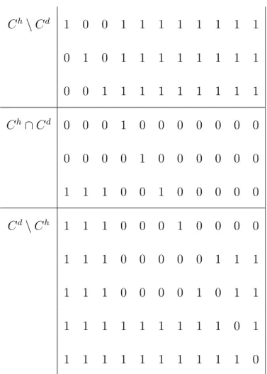
Ch_\_Cd ₁ ₀ ₀ ₁ ₁ ₁ ₁ ₁ ₁ ₁ ₁ 0 1 0 1 1 1 1 1 1 1 1 0 0 1 1 1 1 1 1 1 1 1 Ch∩Cd 0 0 0 1 0 0 0 0 0 0 0 0 0 0 0 1 0 0 0 0 0 0 1 1 1 0 0 1 0 0 0 0 0 Cd\Ch 1 1 1 0 0 0 1 0 0 0 0 1 1 1 0 0 0 0 0 1 1 1 1 1 1 0 0 0 0 1 0 1 1 1 1 1 1 1 1 1 1 1 0 1 1 1 1 1 1 1 1 1 1 1 0 Table 3.2: Affinely Independent Points

inequalities are the theoretically strongest inequalities. To prove that M V M CI_Ch_,Cd_,2 3 is

facet defining one must show that its face has dimension 10.

The dimension is bounded by the number of affinely independent points in the face. There are 11 such affinely independent points, because the conditions of Theorem 3.2 are satisfied. These 11 points are given in Table 3.2. The following discussion proves these points are in the face and are affinely independent. It also provides additional insight into this theorem. Note that the lines in Table 3.2 are there to assist with understanding of the different indices in the sets Ch_\_Cd_, _Ch_∩_Cd_{, and} _Cd_\_Ch_.

(41)

A critical assumption in Theorem 3.2 is that there was a tie in the smallest α value. In this case, observe that MVMCA has two iterations where α0 ₌ 2

3. One case hascounth= 1

and countd = 6, and the second case has counth= 3 and countd = 3. For the assumptions of Theorem 3.2, let (counth1, countd1) = (1,6) and (counth2, countd2) = (3,3).

The setSi ={ihd1 , i hd |Ch_\_Cd_|−_counth 1+2, ..., i hd |Ch_\_Cd_|}∪{i d |Cd_|−_countd 1+1, ..., i d |Cd_|}={1,6,7,8,9,10,11}

is not a cover. Thus, condition i) is true and the point in the first column in Table 3.2 is feasible. Since a1 ≥ a2 ≥ a3, the points in the second and third column are also feasible.

Each of these points is in the face because 1 +2₃ ∗6 = 5, which is a direct result of choosing counth1 variables associated with indices in Ch \Cd and countd1 variables associated with

indices in Cd.

The setSiii ={ihd_|_Ch_\_Cd_|−_counth

2+1, ..., i hd |Ch_\_Cd_|}∪{i d 1, i d |Cd_|−_countd 2+2, ..., i d |Cd_|}={1,2,3,4,10,11}

is not a cover. Thus condition iii) is true and the point in the fourth column in Table 3.2 is feasible. Since a4 ≥a5 ≥a6 ≥a7, the fifth, sixth and seventh columns are feasible points

also. These points all have corresponding counth= 3 and countd= 3 and thus they are in M V M CI_Ch_,Cd_,2

3’s face.

The setSiv ={ihd_|_Ch_\_Cd_|−_counth

2+1, ..., i hd |Ch_\_Cd_|} ∪ {i d |Cd_|−_countd 2, ..., i d |Cd_|−₁}={1,2,3,8,9,10}

is not a cover. Thus condition iv) is true and the point in the eleventh column of Table 3.2 is feasible. Because a8 ≥a9 ≥a10 ≥ a11, the eighth, ninth and tenth columns in Table 3.2

are feasible points. Again these points all have corresponding counth = 3 and countd = 3 and are in the face of M V M CICh_,Cd_,2

3. Thus, these are 11 points that are feasible and on

the desired face.

(42)

Furthermore, Ch∪Cd =N and condition v) is also vacuously true.

To prove that these 11 points are affinely independent, observe that the first 3 points only have a single 1 in each of the first 3 rows. Thus, this set of points is affinely independent.

Now consider the fourth through eleventh points. The fourth to seventh points only have a single 1 in the fourth to seventh row. The eighth through eleventh columns are all constant except for the cyclical permutation of 3 ones over the last four rows. Since 3 and 4 are relatively prime, these points are affinely independent. Consequently, the fourth through eleventh points are affinely independent.

Since (1,6) is affinely independent from (3,3); these two sets of points are also affinely independent. Thus, these points are affinely independent, the face ofM V M CI_Ch_,Cd_,2

3 has a

dimension of 10, and this face is a facet of conv(PKP).

Now that MVMCA has been shown to produce a facet defining inequality, it is necessary to show that this type of inequality could not have been obtained using any other method currently in use and also needs to be shown that it is not simply a slight variation on an existing strategy of finding cutting planes for the knapsack problem.

As mentioned in the introduction, Hickman and Easton’s [24] work on merging inequali-ties was the catalyst to this research. Their method can only merge on a single variable and could not create M V M CI_Ch_,Cd_,2

3. Furthermore, MVMCA would generate stronger

inequali-ties even if|Ch∩Cd|= 1. That is, MVMCA would generate an α coefficient that is at least as large as the _|_Cd1_|−₁ scaling coefficient generated by Hickman and Easton’s method.

(43)

generates integer coefficients. Thus, starting with theCh cover inequality and lifting sequen-tially could not create M V M CI_Ch_,Cd_,2

3. If M V M CICh,Cd, 2 3 is multiplied by 3 2, it becomes 3 2x1+ 3 2x2+ 3 2x3+x4+x5+x6+x7+x8+x9+x10+x11≤ 15

2. Clearly, this is not a sequentially

lifted version of the Cd donor inequality. Consequently, sequential lifting cannot generate this M V M CI_Ch_,Cd_,2

3.

Simultaneous lifting could theoretically generate M V M CI_Ch_,Cd_,2

3 if given the correct

initial valid inequality and the proper lifting weights. This inequality could be generated by starting with either of the valid inequalitiesx1+x2+x3 ≤5 orx4+x5+x6+x7+x8+x9+

x10+x11 ≤ 15₂ . Neither of these inequalities are tight and both inequalities can be trivially

strengthened tox1+x2+x3 ≤3 and x4+x5+x6+x7+x8+x9+x10+x11≤7. Thus, without

consulting an oracle one could not generateM V M CI_Ch_,Cd_,2

3 with simultaneous uplifting.

Finally, numerous other methods exist to find valid inequalities. Such methods as Chvatal-Gomory cuts [9], mixed integer rounding cuts [12], superadditive cuts [18] and mod-ular cuts [17] may be able to generate M V M CICh_,Cd_,2

3, but not without substantial effort

and possibly the consultation of an oracle. Thus, MVMCIs are a new class of cutting planes for the knapsack polytope.

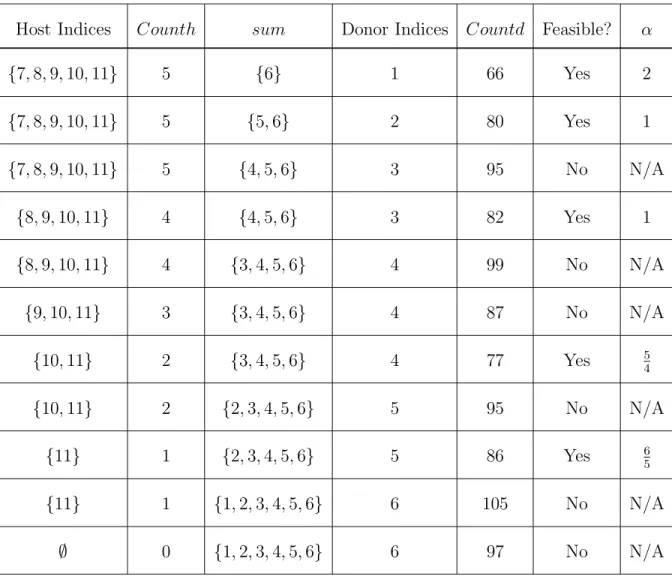
After the implementation of MVMCA on an example, it is prudent to show that MVMCA could also be run by reversing the donor and host covers. Thus letC0h={6,7,8,9,10,11,12}

and C0d ₌_{_1,_2,_3,_4,_5,₆_}_{. Table 3.3 provides a summary of the loops of MVMCA.}

MVMCA returns α equal to 1, thus the valid inequality isM V M CIC0d_,C0h_,₁ =

P11

i=1xi ≤

7. This inequality is merely an extended cover inequality. In this particular case, little is gained from MVMCA. However, if one reduced the right hand side of the knapsack constraint

(44)

Host Indices Counth sum Donor Indices Countd Feasible? α {7,8,9,10,11} 5 {6} 1 66 Yes 2 {7,8,9,10,11} 5 {5,6} 2 80 Yes 1 {7,8,9,10,11} 5 {4,5,6} 3 95 No N/A {8,9,10,11} 4 {4,5,6} 3 82 Yes 1 {8,9,10,11} 4 {3,4,5,6} 4 99 No N/A {9,10,11} 3 {3,4,5,6} 4 87 No N/A {10,11} 2 {3,4,5,6} 4 77 Yes 5₄ {10,11} 2 {2,3,4,5,6} 5 95 No N/A {11} 1 {2,3,4,5,6} 5 86 Yes 6₅ {11} 1 {1,2,3,4,5,6} 6 105 No N/A ∅ 0 {1,2,3,4,5,6} 6 97 No N/A

(45)

to 79, then theαvalue reported from MVMCA would have been 5₄ and it would have resulted in an inequality that is stronger than an extended cover inequality.

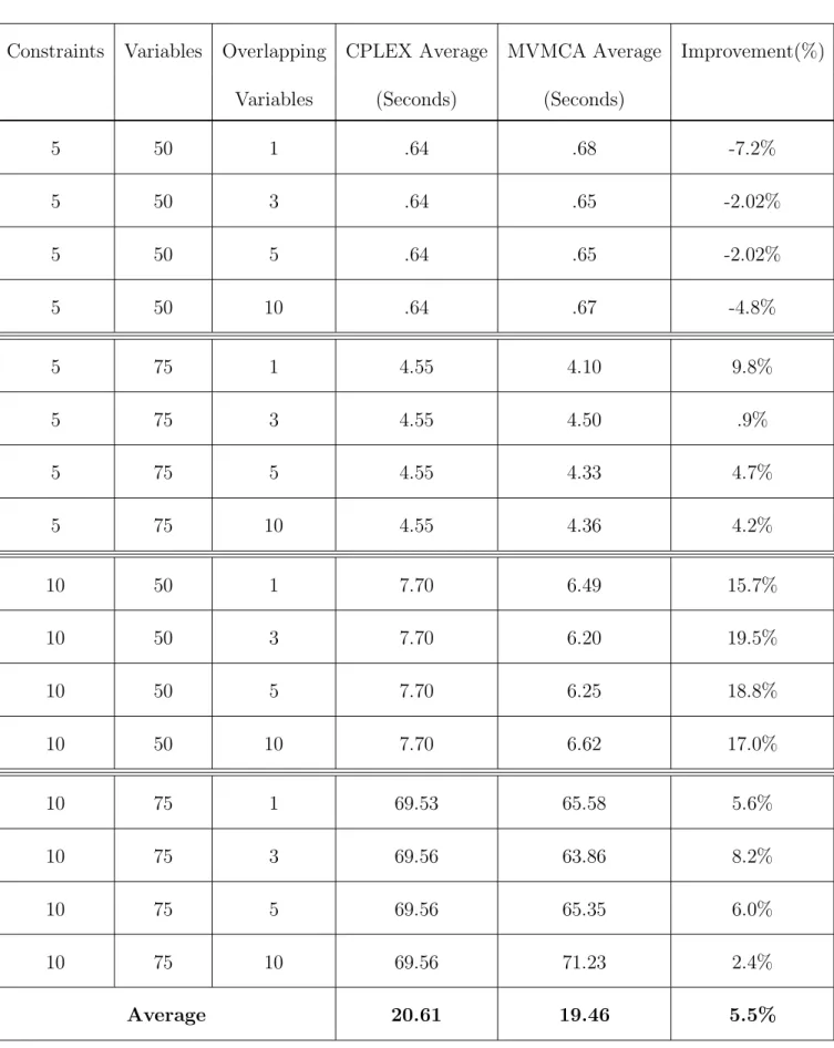
To demonstrate the impact of MVMCA in more complicated examples, Chapter 4 presents a computational study. This study performs multiple runs with several examples of MVMCA being implemented on varying sizes of MK instances. Once the best strategy is chosen larger problems are solved to show the usefulness of MVMCIs.