Comparison and Evaluation of Didactic Methods in Numerical Analysis for the Teaching of Cubic Spline Interpolation

(1)

Comparison and Evaluation of Didactic Methods in Numerical

Analysis for the Teaching of Cubic Spline Interpolation

Abtihal Jaber Chitheer

supervised by Prof. Dr. Carmen Ar´evalo

(2)

(3)

Abstract

Faculty of Science

Centre for Mathematical Sciences Numerical analysis

Master in Science

Comparison and Evaluation of Didactic Methods in Numerical Analysis for the Teaching of Cubic Spline Interpolation

by Abtihal Jaber Chitheer

In mathematical education it is crucial to have a good teaching plan and to execute it correctly. In particular, this is true in the field of numerical analysis. Every teacher has a different style of teaching. This thesis studies how the basic material of a particular topic in numerical analysis was developed in four different textbooks. We compare and evaluate this process in order to achieve a good teaching strategy. The topic we chose for this research is cubic spline interpolation. Although this topic is a basic one in numerical analysis it may be complicated for students to understand. The aim of the thesis is to analyze the effectiveness of different approaches of teaching cubic spline interpolation and then use this insight to write our own chapter. We intend to channel every-day thinking into a more technical/practical presentation of a topic in numerical analysis. The didactic methodology that we use here can be extended to cover other topics in numerical analysis.

(4)

(5)

Acknowledgements

I would like to express my gratitude towards my country Iraq for the scholarship. I would like to thank Lund University for giving me the opportunity to do my master degree. I would like to thank my supervisor Carmen Ar´evalo for giving me this opportunity to do my master thesis in the field of numerical analysis and for the guidance and support throughout the process. I would like also to thank the department of Mathematics for feedback and encouragement. Finally I am very grateful for support from my loving family and friends.

(6)

(7)

Introduction

Many problems in mathematics can be presented in several different ways, but all lead us to the same results. Most problems are complex problems, that might be difficult for students to understand. When I was working in Iraq as a mathematics teacher during the years of 2009-2013 I realized that different ways of teaching will affect the students’ level of understanding. Piecewise polynomial interpolation is one topic that students find especially difficult to un-derstand, so we would like to find didactic strategies for teaching this subject. The topic of cubic spline interpolation is a basic topic in the course of numerical analysis and yet students have difficulties in following the process of the construction of a cubic spline based on the conditions a spline must satisfy.

These problems are solved numerically, usually with the help of computers and thus learning how to program this process is also a skill students must develop.

1.1 Aim of the thesis

A mathematical object or concept can be introduced by different sets of equivalent definitions and examples. One fundamental question in this context is that of what teaching method to use. Reading several books on a common topic makes one realize how different similar teachings can be, in style and requirements towards a student. Our goal, in this work of comparison, is to analyze the effectiveness of different approaches and teachings of some particular topics through different course materials, and how to compare and decide between different books with future work in Iraq in mind.

Eventually, the aim of this work is to channel every-day thinking towards a more technical-practical thinking at an earlier stage so that, as a teacher, one can get the expected results from the teaching of a particular topic.

1.2 Spline interpolation

Here we chose to focus on the teaching of spline interpolation. The choice of this topic has two main motivations. First of all, it is one of the basics of numerical analysis. Using an example that is easily understandable by undergraduate students of mathematicians makes the point of the thesis easier to illustrate. Secondly, there are many differences in views and

(10)

the teaching of this subject, and the study of these differences helps to reach the goal of this thesis. Diversity in teaching strategies gives us tools to reach our goal.

1.3 Didactic reflection:

Variation theory of learningwas developed by Ference Marton of the University of Gothenburg in 1997. This theory says that for a teacher to be able to help a student understand a topic, the teacher must first identify the critical aspects of the topic. Once this is done, by varying one aspect while keeping other aspects fixed, the student will learn by observing the differences. Variation theory can be interpreted as “how the same thing or the same situation can be seen, experienced or understood in a limited number of qualitatively different ways” [Maghdid, 2016]. For example, we apply variation theory when we propose several problems that can be solved with the same technique, or when we have one example that can be solved in several different ways. In our development of a chapter for the teaching of cubic spline interpolation we will apply this strategy to try to reach a successful didactics method.

1.4 Additional notes

The four books we have chosen to work with are well-known and used often in the teaching of numerical analysis.

Our goal is not to describe one perfect way of teaching, but to hierichize the methods and teaching strategies by their efficiency.

Any student with basic knowledge of numerical analysis can read this thesis. As we have stated before, our point is not the mathematical aspects but the didactics. Therefore, a basic knowledge is enough and necessary in order to understand most of our points and examples, which will only be clearer if the reader has studied spline interpolation in the past. Furthermore, any person interested in the teaching of mathematics may be interested in reading this work, as successful teaching results from a critical point of view, and especially a self-critical one.

I am a former student of the Department of Mathematics at Mustansiriya University, Iraq, where I have obtained a Bachelor’s degree in theoretical mathematics. I was then employed as a mathematics teacher in the schools Fatima Zahra and Ishtar, where I was often confronted with student complains about the lack of easy accessibility to concepts in theoretical mathematics. Their abstract aspect and the specificity of their applications made students unable to identify their own errors when obtaining incorrect solutions to a problem. I therefore got very drawn into constructing proofs and solutions that were more interesting and transparent. I aspire to develop a better teaching method, more comfortable for both teachers and students, by, for example, privileging illustration over expansive calculations.

(11)

Analysis of four different

approaches to the teaching of

splines

In this thesis I have compared the presentation of the topiccubic splines from four different Numerical Analysis books intended to be used as textbooks in regular undergraduate courses.

2.1 Comparison criteria

The four numerical analysis books present the topic under study in considerably different ways. In order to understand their similarities, differences, weaknesses and strengths, we will use the following key points as comparison criteria: insertion point, teaching structure, and

outcome procurement. Analysis of the structure of teaching is a logical requirement to explain different effectiveness in teaching outcome. To understand the way an author argues we have to take specific study and comparison criteria. These key points are as follows:

1. Insertion point: Here we will focus on how the author introduces the concept of cubic splines. We will study the ways in which the authors motivate and direct the reader to cubic splines. For example, how was the presentation initiated? What are the different types of interpolation that are described before starting the cubic spline section? How is the previous material on interpolation used to connect to this subject?

2. Teaching structure: This part is divided into two subsections. Firstly, we touch on the

Introduction process. What are the key points in the initial presentation of cubic splines? What was the strategy for developing the important concepts in the topic? Secondly, we look at at the elaboration process. In this part we study how the authors expand on the topic, developing each point so that there is a line of development throughout. For example, how is the derivation of cubic splines done? How many end conditions are mentioned? Were there any Theorems mentioned or were the explanations of a more informal type?

3. Outcome procurement: This part deals with the conclusions of the presentation of the subject. For example, were there examples and applications that clarified the concept

(12)

Insertion Point Teaching Structure Introduction Outcome Procurement Comparison criteria Elaboration 3 2 1 2.1 2.2

Figure 2.1: Scheme of the comparison criteria keys

of cubic splines? Are there exercises that allow the reader to test his understanding of cubic splines? Were there any summaries at the end of the presentation?

Using these criteria we will be able to study and analyze each book in a systematic manner so that we can use this knowledge in the next chapter to compare the four books and evaluate their didactic methods. The comparison will be made in the form of questions and answers, and this will allow us to go on to the evaluation of the books. Finally, using the results of previous chapters we will come with our conclusion and suggest a didactic method for this topic.

The tables and plots shown in the presentation of the books in the following subsections were taken directly from the books themselves. The last section of the thesis, theAppendix, displays a copy of the chapters or sections that have been mentioned in this thesis. This was done in order to make it easier for the reader to compare the original versions with the thesis.

2.2 Book descriptions

The analysis of each book will start with a schematic representation of how the subject of cubic splines is presented and developed. This will be done by using the key comparison criteria mentioned before, that is,insertion point, teaching structure, andoutcome procurement. We will then go on to explain each section in detail.

2.2.1 Book I: Applied Numerical Methods with MATLAB for Engineers

and Scientists by Steven C. Chapra, 2011.

Steven C. Chapra is professor at the Department of Civil and Environmental Engineering at Tufts University in Massachusetts, U.S.A. He specializes in environmental engineering.

This book focuses on applied numerical analysis using MATLAB. The book can be used for teaching at a basic level and at a more advanced level, and Chapra’s book is widely used

(13)

Figure 2.2: Steven C.Chapra, author of the bookApplied Numerical Methods with MATLAB for Engineer and Scientists, 2011.

as textbook in different countries. For example, Florida University ([University of Florida, 2009]) in the United States has been using this book for the courseIntroduction of Numerical

Methods of Engineering Analysis. McMaster University in Canada recently used Chapra’s

book as textbook in the courseComputer Engineering 3 SK3 Numerical Analysis ([McMaster University, 2014]), and Hacettepe University in Turkey uses this book as textbook in the courseNumerical Analysis with MATLAB ([Hacettepe ¨Universitesi, 2017]). In Italy, it is also used for the course Numerical Methods at the online Universita Telematica Internazionale

UNINETTUNO. The topic of cubic splines is a 10-page section in the chapterSplines and

Piecewise Interpolation. Cubic Splines is mentioned as the last type of spline interpolant and this section also includes a primer on piecewise interpolation in MATLAB.

2.2.1.1 Insertion Point

The chapter titled Splines and Piecewise Interpolation in Chapra’s book is grounded on its preceding chapter, Polynomial Interpolation, where Runge’s function was introduced as an example of the dangers of higher-order polynomial interpolation. The motivation starts by mentioning the problems observed in the previous chapter with higher degree polynomials, but without any reference to Runge’s function example. In addition, the author proposes an alternative solution to this problem by using piecewise lower order polynomials (spline functions).

The chapter on splines and polynomial interpolation is opened with an example. When a function varies sharply at a point, interpolation polynomials of high degree induce undesired oscillations. This problem is illustrated in Figure 2.4. A linear 3-piece polynomial, as shown in (d), does a much better job that the polynomials of degree 3, 5 and 7, shown in (a, b, c).

The notion of splines is introduced as piecewise lower-order interpolating polynomials, and they are suggested as an alternative to higher-order polynomials when the function to interpolate has local, abrupt changes.

After presenting the reader with a motivation to study splines, the author gives a historical account of spline construction. In order to “draw smooth curves through a set of points” when a plan for some construction was drafted, a thin, flexible strip (called aspline) was used. The author points to Figure 2.5 to illustrate that the data point (pins) are “interpolated” by

(14)

Book I Chapra

Natural Splines end conditions Quadratic Splines Introduction to Splines Linear Splines 1.1 1.2 1.3 Piecewise Interpolation in MATLAB Table lookup 1.2.1 1.5 Insertion Point Derivation of Cubic Splines Clamped end condition Not-a-Knot end condition 1.4.2 End Conditions 1.4.3 Cubic Splines General formula and

properties Teaching Structure 1.4 Elaboration End conditions Introduction Outcome Procurement  Computer codes  Examples  Exercises  Case Study

Figure 2.3: Schematic content and organization of Chapter 18, ”Splines and Piecewise Inter-polation” in Chapra’s book [Chapra, 2011].

(15)

(16)

Figure 2.5: Illustration of an early use of splines to construct smooth curves passing through pre-defined points (Chapra [2011], p. 431).

Figure 2.6: This figure displays the notation used to derive splines (Chapra [2011], p. 432).

smooth curves as the strip goes through the pins. In fact, the author asserts that these curves are in fact cubic splines.

At the end of his introductory section, the author gives an overview of the topics that he will discuss in the remainder of the chapter.

Linear Splines

The section onlinear splines starts with a detailed description of the notation, as portrayed in Figure 2.6.

Firstly, the reader is asked to observe thatndistinct data points generaten−1 intervals. It is then shown that for each intervalithere is a spline functionSi(x), and that a linear spline has a straight line connection between the two end points of the intervals. Thus, it is easy to formulate the equations for these splines. Then, the practical aspect of this formulation

(17)

Figure 2.7: (a) Linear spline, (b) Quadratic spline, (c) Cubic spline, with a cubic interpolation polynomial, ([Chapra, 2011, p. 433].

is exposed: they can be used to evaluate the function at any point in the interval containing the data points. The author explains that there are two steps in doing so: (1) locate the subinterval where the point lies, and (2) use the appropriate equation to evaluate the spline. An example is given to illustrate these steps.

Chapra points out that using linear splines is equivalent to “using Newton’s first-order polynomial to interpolate within each interval”. An example shows the first-order spline, the second-order spline, and the cubic spline interpolations of four data points (Figure 2.7). The aim of Figure 2.7, is to demonstrate that the same data points can be interpolated by splines of different orders: a linear spline, a quadratic spline, and a cubic spline, and that the resulting splines will yield different function evaluations. It also introduces the concept of smoothness of a curve, and its relation to its derivatives.

Here another new concept is introduced: aknot is defined as a data point where two spline pieces meet. The author indicates the main disadvantages of linear splines:

1. First-order splines are not smooth.

2. The slope changes abruptly where the spline segments meet (knots). 3. The first derivative of the function is discontinuous at these specific points.

(18)

Figure 2.8: Table (17.7) from the previous chapter, showing air density at different tempera-tures (Chapra [2011], p. 406).

The disadvantage of the non-smoothness of linear splines is a motivation why it is impor-tant to consider higher-order splines. Nevertheless, the author states that linear splines are important in their own right, and gives an example of their usefulness.

Table Lookup

Chapra uses the example of a table lookup to show why linear spline interpolation may be useful. The idea is to interpolate values from a table of independent and dependent variables. “For example, suppose that you would like to set up an M-file that would use linear interpo-lation”, if programming in MATLAB, with specific data that you have as a table, for example Table 2.8.

Given such a table, to perform a linear interpolation at a particular value of the independent variable, the subinterval containing the required value must be found. The action of finding the appropriate values in the table is calledtable lookup. Here the author explains in detail how to construct a Matlab file that does the interpolation task. He describes the process in two steps:

1. search of the interval where the independent variable is located, and 2. linear interpolation.

The first step is described in detail, and two different types of search are presented: a sequential search, for a small set of data points, and a binary search, for large sets of data.

The next section takes on the aspect of the continuity of the derivatives of the interpolating function.

Quadratic Splines

The author starts this section by claiming that in order to haven-the continuous derivatives, a spline must be of degreen+ 1 or higher. Then he asserts that the most frequently used splines are the cubic ones, because higher derivative discontinuities at the knots in most cases cannot

(19)

be observed visually. Even though the author’s aim is to discuss cubic splines, he chooses to go through the derivation ofquadratic splines because this derivation is less complicated.

The derivation of quadratic splines is done in detail in order to show what are the important points that must be taken into account. It starts by giving the general form of each spline segment as a quadratic polynomial centered at the starting point of each subinterval,

Si(x) =ai+bi(x−xi) +ci(x−xi)2 (2.1) Then it proceeds to count the number of intervals, equations, and unknowns, which must correspond to the number of coefficients of the spline. Finally, it gives the conditions that must be satisfied by the unknowns. These conditions are continuity conditions, interpola-tion condiinterpola-tions and end conditions. By counting the number of continuity and interpolation conditions, it is clear that there must be one end condition so that the number of equations (conditions) equals the number of unknowns.

Finally, an example is given (Example 18.2 in the book) to illustrate this construction. This example uses the same data as the previous example in the section for linear splines. In addition, it refers the reader to Figure 2.7, where (b) shows this quadratic spline, and points to the fact that a straight line connects the first two data points due to the end condition, and also that the curve for the last interval swings too high. These observations serve as a motivation to study cubic splines, as they do not exhibit this undesired behaviour.

2.2.1.2 Teaching Structure

This section is divided into two parts. Firstly, thePresentation part refers to the introduction of the basic material defining cubic splines. Secondly, theElaboration part contains further details about cubic splines.

Introduction

The author starts by restating the disadvantages of using linear or quadratic splines, and then states that higher degree splines tend to exhibit inherent instabilities, while cubic splines “exhibit the desired appearance of smoothness” while providing the simplest representation. The steps in which the author displays cubic splines follow the lines of his exposition for quadratic splines:

1. General form ofcubic splines.

Si(x) =ai+bi(x−xi) +ci(x−xi)2+di(x−xi)3 (2.2) 2. Number of intervals, unknowns, and continuity and interpolation conditions.

3. Calculation of the number of end conditions that need to be added, and what formula-tions they can have.

4. Enforcement of the continuity and interpolation conditions.

5. Discussion of the several options for end conditions. One type of end condition is, for example, the conditions for a natural spline, which can be observed in Figure 2.5. Additionally, to complement the choice of several options, the author adds two more options of end conditions which are described in Section 18.4.2 of the book.

(20)

6. Enforcement of the end conditions.

In the next section we present the details of the derivation of cubic splines in Chapra’s book.

Elaboration

There are two main issues in the construction of cubic splines. Firstly, the derivation of cubic splines from the continuity and interpolation conditions. Secondly, the enforcement of end conditions.

Derivation of Cubic Splines

A major reason for the introduction and derivation of quadratic splines was to pave the way to the derivation of cubic splines. Correspondingly, also here the number of conditions and the number of unknowns are determined, and it is shown that two additionalend conditions

are required. The construction of cubic splines is demonstrated step by step.

1. The formula for acubic spline (third-order polynomial for each interval between knots) is given. This formula is centered around the initial point of each subinterval.

2. The interpolation and continuity conditions for thecubic splineat the knots are enforced. 3. The continuity conditions for the first derivative of the cubic spline at the knots are

enforced.

4. The continuity conditions for the second derivative of thecubic spline at the knots are enforced.

5. The result obtained in the previous steps are substituted into the original formula, yielding a set of equations containing only the unknowns corresponding to the coefficients of the quadratic terms of the spline sections. These equations hold for all the internal knots.

6. The two end conditions are added to the system. As an example, the conditions taken are those for a natural spline, i.e., that the second derivative of the spline is equal to zero at the endpoints.

7. The linear system is shown in a matrix-vector form, showing that the system matrix is tridiagonal.

Finally, an example of the construction of a natural cubic spline is shown in [p. 442] of Chapra’s book ([Chapra, 2011]). The author provides the same data that was used for linear and quadratic splines, and the results are displayed in Figure 2.7.

The first type of end conditions applied to cubic splines resulted innatural splines. In the next section, the author describes other end conditions.

(21)

Figure 2.9: How to specify different end conditions (Chapra [2011], p.443 ).

I: Natural End Condition

As described earlier, a natural spline is defined by requiring that the second derivatives at the two endpoints are equal to zero. This type of spline results when the drafting spline is allowed to behave naturally, without constraining it at its endpoints.

II: Clamped End Condition

Clamped splines result when a drafting spline is clamped at its ends. The first derivative is specified at the two ends.

III: Not-a-Knot End Condition

This condition implies that the third derivative is required to be continuous at the second and the next-to-last knots. Because the spline segments are cubic polynomials, this condition implies that the first and second segments are a single polynomial, and so are the last and next-to-last segments. Thus, these knots are not true knots any longer.

Table 2.9 shows how to modify the first and last equations in order to construct natural,

clamped and not-a-knot splines. Figure 2.10 shows the different end conditions by using the same example that was mentioned last section.

2.2.1.3 Outcome Procurement

In the next section the author describes how the user can take advantage of some of Matlab’s built-in functions for piecewise interpolation. Two problems are solved as examples. Some snippets of code are given, and the results are plotted.

Piecewise Interpolation in MATLAB

(22)

Figure 2.10: Using the data of the previous example, splines withnatural,clamped and not-a-knot end conditions are plotted (Chapra [2011], p. 444).

(23)

Figure 2.11: Runge’s function with nine data points constructed in MATLAB by using a “not-a-knot” end condition ([Chapra, 2011, p. 445]).

(24)

Figure 2.12: Runge’s function with nine data points constructed in MATLAB by using a clamped end condition (Chapra [2011], p. 446).

(25)

Figure 2.13: Discrete data fitted with (a) a first degree spline (b) a zero degree spline (c) a standard spline (d) an Hermite spline (Chapra [2011], p. 448).

(26)

Figure 2.14: Timothy Sauer, author of the book Numerical Analysis, 2012.

1. The spline function implements cubic spline interpolation. The author describes the syntax and explains how to choose different end conditions. He then uses Runge’s function, already mentioned in the previous chapter (example 17.7), to show how the use of different cubic splines remove the oscillations caused by the Runge phenomenon. The results using different end conditions are presented in Figures 2.11 and 2.12. 2. The functioninterp1implements spline and Hermite interpolation and also other types

of piecewise interpolation. Here is an easy way to implement “a number of different types of piecewise one-dimensional interpolations” with a given general formula. There are four different optional functions: nearest (for nearest neighbor interpolation),linear (for linear interpolation), spline(for piecewise cubic spline), andpchip(for piecewise cubic Hermite interpolation). Finally, an example is presented to illustrate the trade-offs of using interp1, as shown in Figure 2.13.

After having presented the subject ofcubic splines in detail the author solves a particular real-life heat transfer problem by using cubic splines. The solution is presented in great detail ([Chapra, 2011], p. 452–456).

2.2.2 Book II: Numerical Analysis by Timothy Sauer, 2012.

Timothy Sauer is professor of mathematics at George Mason University. He specializes in dynamical systems.

This book is intended for students of engineering, science, mathematics, and computer science. The book offers an introductory level with some more advanced level topics, and uses MATLAB for its computer examples. Sauer’s book is used as textbook in many countries. For example, Washington State University used this book as textbook in the course Numer-ical Analysis during spring 2017 ([Washington State University, 2017]). Lund University in Sweden used it as textbook for its course Numerical Analysis for Computer Science during spring 2017 ([University, 2017]). At Harvard university in Cambridge, Massachusetts, it was used in the 2012 course Numerical Analysis ([Harvard University, 2012]). The topic ofcubic splines covers a 14-page section of the chapter on Iterpolation.

(27)

Book II Sauer Properties of splines 1.1 Endpoint conditions 1.2 Clamped Cubic Spline Curvature- Adjusted Cubic Spline Not-a-Knot Cubic Spline

Insertion Point Linear Splines

Introduction to Cubic Splines

Natural Splines

Derivation of cubic splines

Cubic Splines 1 Outcome Procurement  Computer codes  Examples  Exercises Teaching Structure Parabolically Terminated Cubic Spline Introduction Elaboration Cubic Splines

Figure 2.15: Schematic content and organization of Chapter 3, Section 4,“Interpolation – Cubic Splines” in Sauer’s book Sauer [2012].

(28)

Figure 2.16: (a) Linear spline interpolation (b) cubic spline interpolation (Sauer [2012], p.166).

2.2.2.1 Insertion point

In Sauer’s book cubic splines are presented as a section of the chapter titled Interpolation, after the sections titled Data and Interpolating Functions, Interpolation Error and Cheby-shev Interpolation. After cubic splines there is a section on B´ezier curves. In the chapter

Interpolation Error the author displays the famous Runge phenomenon and uses it to

mo-tivate Chebyshev interpolation, but does not mentioned it in the section for cubic splines. Instead, the author asserts that “splines represent an alternative approach to data interpola-tion” (Sauer [2012]), and the idea of splines is to “use several formulas, each with a low-degree polynomial, to pass through the data points” (Sauer [2012]). The first example of these ideas is given by providing an example (four data points) together with a solution that uses the child game concept of “connecting the dots”, shown in Figure 2.16. The definition oflinear splines is introduced only by working out the formulas for this particular example.

The lack of smoothness of linear splines is pointed out, and this fact allows the author to introduce cubic splines: “cubic splines are meant to address this shortcoming of linear splines” (Sauer [2012]). We are given the equations that define a cubic spline passing through the same given data points, and shown the difference between linear and cubic splines in Figure 2.16. At this point the notion of knots is introduced. The author also mentions an important difference between linear splines and cubic splines:

1. There is obviously one and only one linear spline passing throughndata points. 2. There are infinitely many cubic splines passing through n data points. Consequently,

interpolation cubic splines need extra conditions to be uniquely defined: “extra condi-tions will be added when it is necessary to nail down a particular spline of interest” (Sauer [2012]).

(29)

2.2.2.2 Teaching structure

The reader is firstly introduced to the basic idea of “connecting the dots” (Sauer [2012]) and is motivated to the introduction of cubic splines. The author then elaborates the topic with precise definitions and properties of cubic splines. Finally, end conditions are introduced, and this leads to the discussion of several different types of cubic splines.

Introduction

The author starts by giving a precise definition of cubic splines. First, he gives the general form of a cubic spline passing through the points (x1, y1), . . . ,(xn, yn):

Si−1(x) =yi−1+bi−1(x−xi−1)+ci−1(x−xi−1)2+di−1(x−xi−1)3 x∈[xi−1, xi], i= 1, . . . , n−1 Then, he gives three properties that a cubic spline must satisfy:

1. Property 1: Si(xi) =yi and Si(xi+1) =yi+1 for i= 1, ..., n−1. 2. Property 2: S_i0₋₁(xi) =S 0 i(xi), i= 2, ..., n−1. 3. Property 3: S_i00₋₁(xi) =S 00 i(xi), i= 2, ..., n−1.

The first property is linked to interpolation, while the other two are linked to continuity. Sauer ends his initial presentation by studying the numerical example he gave in the introduction of the topic, and demonstrates that it satisfies the stated properties.

Elaboration

To show how to construct a cubic spline from a set of data points, the author starts by counting the number of conditions and the number of unknown coefficients. He finds the system of equations is underdetermined, because there are two more unknowns than equations, and states that it is important to arrive at a system containing as many equations as unknowns. It is therefore necessary to add two extra conditions.

Sauer states that while there is an infinite number of ways to add two equations to the system, the easiest way is to require the splineS(x) to have an inflection point at each end of the defining interval [x1, xn]. Thus, a new property is added:

• Property 4a: S₁00(x1) = 0 and S_n00₋₁(xn) = 0.

Splines that satisfy this last condition are called natural splines. The conditions that de-fine a spline can be written as a linear system ofnequations innunknowns. These unknowns are the coefficients of the quadratic terms of the spline. The resulting system matrix is strictly diagonally dominant, which means that the system has a unique solution, as stated in the following theorem (Sauer [2012], p. 107):

Theorem 2.10: If the n×nmatrix Ais strictly diagonally dominant, then A is a nonsingular matrix.

Once these coefficients are computed, the remaining ones may be calculated by explicit formulas derived from the continuity and interpolation conditions. Then, the author comple-ments the explanation with a pseudo code that calculates the coefficients of a natural cubic

(30)

Figure 2.17: As shown above four types of end conditions are demonstrated: (a) Natural cubic spline (b) Not-a-Knot cubic spline (c) Parabolically terminated cubic spline (d) Clamped cubic spline [Sauer, 2012] p.173.

spline, given a set of interpolation points (knots). The use of this code is then illustrated by the calculation of a cubic spline passing through three given points. Finally, he presents a MATLAB code that generates a natural cubic spline and that may be modified to include several other types of cubic splines by choosing different end conditions. This is a topic that will be elaborated in the next section.

The author dedicates a new subsection to the analysis of end conditions. He justifies the addition of end conditions by arguing the need of a square system of equations for the determination of the spline coefficients. The first end condition led tonatural splines.

Endpoint conditions

“There are several other ways to add two more conditions” (Sauer [2012]) the author has stated. This observation may support the choice of other options. As natural splines con-ditions occur at the left and right ends of the spline, they are called end conditions. The author notes that there can be many versions of Property 4a, that is, many different sets of

(31)

end conditions. The most popular ones are presented.

Property 4a: Natural spline. A cubic interpolatory splineS(x) is callednatural cubic splines if

S₁00(x1) = 0 , S_n00−1(xn) = 0.

The author already mentions natural splines in the previous section, after presenting the properties of cubic splines, by addingnatural splines as a fourth property, “Property 4a”.

The follows theorem states the uniqueness of a natural cubic spline:

Theorem 3.7: Letn≥2. For a set of data points (x1, y1), . . . ,(xn, yn) with distinct

xi, there is a unique natural cubic spline fitting the points.

Property 4b: Curvature-adjusted cubic spline.

A cubic interpolatory splineS(x) is called acurvature-adjusted cubic spline if

S₁00(x1) =a , S_n00−1(xn) =b.

In the first alternative to natural cubic splines, the user chooses the values of the second derivatives at the endpoints. The author observes that this set of conditions possesses the same qualities as those of the natural spline. He shows how the MATLAB code has to be modified to include this type of cubic spline. He also explains that the new spline coefficient matrix has the same structure as the corresponding matrix for natural splines (the matrix is strictly diagonally dominant).

Property 4c: Clamped cubic spline.

A cubic interpolatory splineS(x) is called aclamped cubic spline if

S₁0(x1) =a and S

0

n−1(xn) =b

where a, b are arbitrary values. This is similar to the previous Property 4b, but the first derivative is substituted for the second derivative. The author mentions the important point “the slope at the beginning and end of the spline are under the user’s control” [Sauer, 2012]. He shows how to replace the MATLAB code with the conditions for the clamped cubic spline and he points to Figure 2.17 to show a plot of a spline interpolation whena= 0 and b = 0. He points out thatTheorem 3.7 also holds because the “strict diagonal dominance holds also for the revised coefficient”.

Property 4d: Parabolically terminated cubic spline.

A cubic interpolatory spline S(x) is called a parabolically terminated cubic spline if the first spline polynomialS1 and the last spline polynomialSn−1 are forced to be at most of degree 2. The author claims that when these conditions are applied the system has a strictly diagonally dominant matrix if the dimension of the system is reduced by replacing c1 by c2 and cn by

cn−1. Finally, the author shows how to modify the MATLAB code to include the parabolically terminated spline conditions.

(32)

Property 4e: Not-a-Knot cubic spline.

A cubic interpolatory splineS(x) is called anot-a-knot cubic spline if

S₁000(x2) =S 000 2 (x2) and S 000 n−2(xn−1) =S 000 n−1(xn−1).

SinceS1(x) andS2(x) are polynomials of degree 3 or less, the author explains the require-ments of not-a-knot cubic spline interpolation are equivalent to eliminating the second and the next-to-last knots. “Requiring their third derivatives to agree at x1, while their zeroth, first, and second derivatives already agree there, causesS1 and S2 to be identical cubic poly-nomials” (Sauer [2012]). Therefore, he notes thatx2 is not needed as a base point and that the spline gives the same formula S1 =S2, in all of [x1, x3]. But not only is x2 not need as a base point, but also xn−1. This is evidently no longer a knot. The author explains how the not-a-knot cubic spline conditions can be inserted in the MATLAB code and he points to Figure 2.17 where we can observe a plot of a not-a-knot spline and compare it with that of a natural spline. Finally, the author states Theorem 3.8, which is similar to Theorem 3.7. These Theorems state that a unique solution for each end conditions exists:

Theorem 3.8: Assume thatn≥2. Then, for a set of data points (x1, y1), ...,(xn, yn) and for any one of the end conditions given by Properties 4a-4c, there is a unique cubic satisfying the end conditions and fitting the points. The same is true assuming that

n≥3 for Property 4d andn≥4 for Property 4e.

The section is closed by a short explanation on MATLAB’ssplinecommand, which uses a not-a-knot cubic spline as a default.

The previous section is followed by a list of exercises and computer problems.

The list of exercises includes theoretical as well as more practical questions, such as check-ing whether a set of equations defines a cubic spline, or findcheck-ing a particular type of spline that interpolates a set of given points.

In the computer problems section the reader is asked to find and plot a spline, given a set of interpolation points and end conditions.

2.2.3 Book III: Numerical Analysis: Mathematics of Scientific Computing,

by David Kincaid and Ward Cheney, 2002.

David Kincaid was professor at the Department of Computer Science and at the Institute for Computational Engineering and Sciences at the University of Texas at Austin. His main subjects were iterative methods and parallel computing. Ward Cheney was a professor at the Department of Mathematics at the University of Texas at Austin. He specialized in numerical analysis and approximation theory.

This book is directed to students with diverse backgrounds, and at a more advanced level. Kincaid and Cheney’s book has been used as textbook for higher level courses at several universities. For example, the courseMathematical Numerical Analysis at Duke University in Durham, North Carolina, used this book during spring 2015 ([Duke University, 2015]). Also,

(33)

Figure 2.18: David Kincaid Figure 2.19: Ward Cheney

Figure 2.20: The authors of Numerical Analysis: Mathematics of Scientific Computing, 2002.

this book was used in the course Numerical Analysis and Differential Equation during fall 2016 at Cornell University in Ithaca, New York, and in the courseIntroduction to Numerical

Analysis: Approximation and Nonlinear Equations in 2014 at University of California San

Diego. The cubic spline section in this book is presented at a more advanced level than the other books studied here. The explanations are quite general and only pseudo code is used to describe computer programs. The section on cubic splines is eight pages long.

In Figure 2.21 we give a schematic organization of the chapter oncubic splines in Kincaid and Cheney’s book.

Chapter 6 of this book is titled Approximating Functions. The specific objective of this chapter is to present different types of functions that can be used to approximate other functions or data. The chapter starts with the sections Polynomial Interpolation, Divided Differences,Hermite Interpolation and Spline Interpolation. Each of these sections is mostly self-contained. The authors start the section of Spline Interpolation directly, without any motivation. Instead, they give a formal definition of a spline function of degree k [Kincaid and Cheney, 2002].

To introduce the notion of cubic splines, the authors give the definition of a general spline and then they describe low-degree splines. Then cubic splines are derived, and some theoretic results on optimality are discussed. Then, tension splines are described, and finally higher-degree splines are discussed.

2.2.3.1 Insertion point

Kincaid and Cheney start with definition of a spline function of degreek, defining knots and the continuity conditions.

(34)

Spline Interpolation 1 Introduction Spline of Degree 0 Spline of Degree 1 Problem Set

Book III

Kincaid

and

Cheney

Mention Natural cubic splines Theorem on Optimality of Natural Splines Insertion Point Teaching Structure Cubic Splines Introduction Constrict general formula of cubic spines Elaboration derivation of cubic splines Outcome Procurement

Figure 2.21: Content and organization of Chapter 6, Section 4,“Spline Interpolation” Kincaid and Cheney [2002].

(35)

1. S is a continuous piecewise polynomial of degree at mostk on each subinterval [t0, tn]. 2. S has continuous derivatives of all orders up to k−1.

No interpolation conditions are given, so that the splines are free to interpolate not only at the knots, but at any given points.

The particular definitions ofsplines of degree 0 andsplines of degree 1 are given, together with graphical examples. They do not mention quadratic splines.

The authors present splines of degree 0 as “piecewise constants”,

Si−1(x) =ci−1 x∈[ti−1, ti) , i= 1, ..., n (2.3) The authors remark that the intervals for these splines do not intersect each other and so there is no ambiguity in their definition at the knots. To clarify the case he offers a simple example by looking at a spline of degree 0 with six knots, shown in Figure 2.22:

Figure 2.22: Figure 6.3 shows the spline of degree 0 with six knots and Figure 6.4 shows the spline of degree 1 with nine knots ([Kincaid and Cheney, 2002, p.350]).

For splines of degree 1 the authors start by giving Figure 2.22. The linear splines function formula is defined by:

Si−1(x) =ai−1x+bi−1, x∈[ti−1, ti) (2.4) S(x) =      S0(x) =a0x+b0 x∈[t0, t1) Si−1(x) =ai−1x+bi−1 x∈[ti−1, ti) Sn−1(x) =an−1x+bn−1 x∈[tn−1, tn] (2.5)

(36)

1. How can a spline of degree 1 be evaluated? 2. How can express the functionS on (∞, t1]? 3. How can we express the functionS on [tn−1,∞)?

Finally, the authors present a pseudocode to evaluate a linear spline at a point x when the knots, the coefficients, and the number of subintervals are given. Figure 2.23 shows this code.

Figure 2.23: A pseudocode to evalauate a linear spline function definition by known ti and coefficients (ai, bi) (Kincaid and Cheney [2002], p.350).

2.2.3.2 Teaching structure

Introduction

The notion of cubic splines is introduced by emphasizing that these are the splines most often used in practice.

The authors motivate the topic by giving a table containing a set of data points:

x t0 · · · t1 tn

y y0 · · · y1 yn

A cubic spline that interpolates the data is to be constructed. [Kincaid and Cheney, 2002]. What follows is a step-by-step explanation of how the authors develop cubic splines. It must be noted that the authors assume that the interpolation points are the same as the knots.

(37)

1. The authors describe the spline by its polynomial pieces: S(x) =            S0(x) x∈[t0, t1] S1(x) x∈[t1, t2] .. . ... Sn−1(x) x∈[tn−1, tn] (2.6)

where each Si is a cubic polynomial on [ti, ti+1], and the polynomials interpolate the data points so that

Si−1(ti) =yi=Si(ti) (1≤i≤n−1)

2. The authors discuss the question: Does the continuity requirements onS,S0, andS00 as well as the interpolation conditions provide enough conditions to define acubic spline? Altogether these are 4n−2 conditions for determining 4nunknown coefficients. There-fore, there are two degrees of freedom, “and various ways of using them to advantage” [Kincaid and Cheney, 2002], the authors say.

Elaboration

The authors proceed to the derivation of cubic splines immediately after the introduction. When considering end conditions they only point towardsnatural end conditions, describing it as an “excellent choice”. No other end condition is mentioned. Now the authors explain the derivation of cubic splines and their end conditions.

Derivation of cubic splines

For the derivation of cubic splines the authors use two conventions, 1. The unknowns are defined aszi :=S

00

(ti), i= 0, ...., n. They are used to enforce the continuity condition for second derivative of a cubic spline.

2. The authors use the notationhi:=ti+1−ti.

As the second derivative of a cubic polynomialS_i00 is a linear function, and becauseS_i00(ti) =zi andS_i00(ti+1) =zi+1, it can be written in terms of Lagrange polynomials as

S_i00(x) = zi hi (ti+1−x) + zi+1 hi (x−ti) (2.7)

Integrating twice gives

Si(x) = zi 6hi (ti+1−x)3− zi+1 6hi (x−ti)3+C(x−ti)−D(ti+1−x) (2.8) with integration constantsC andD. Next, the authors show how these can be determined from interpolation and continuity conditions. Firstly,Si(ti) =yi is imposed which gives

D= yi

hi

−zihi 6 .

(38)

Secondly,Si(ti+1) =yi is imposed yielding

C = yi+1

hi

−zi+1hi 6 .

We observe that if thezi were known, thenC andD would be known too, and

Si(x) = zi 6hi (ti+1−x)3+ zi+1 6hi (x−ti)3+ ( yi+1 hi −zi+1hi 6 )(x−ti) + ( yi hi −zihi 6 )(ti+1−x) (2.9) To obtain Equation (2.9) the authors used two conditions:

• limx↓tiS 00

(x) =zi = limx↑tiS 00

(x), which is the continuity condition for S00.

• Si(ti) =yi,Si(ti+ 1) = yi+1, which refers to Si(x) is continuous function when x=ti and x=ti+1

What about the continuity of first derivative S0(x)? The authors observe that “forS0 at the interior knotsti, we must haveS

0

i−1(ti) =S

0

i(ti)” [Kincaid and Cheney, 2002], and so,

hi−1zi−1+ 2(hi+hi−1)zi+hizi+1= 6 hi (yi+1−yi)− 6 hi−1 (yi−yi−1), i= 1, ..., n−1. (2.10)

As these equations result in an underdetermined system, we need to add two more condi-tions. One choice, z0 =zn= 0, results in what is called a natural cubic spline. Writing the linear system results in a matrix that is a tridiagonal and diagonally dominant. The authors show now to solve this system by Gaussian elimination adapted to this structure. The fol-lowing Figure 2.24 shows the pseudo code for theGaussian elimination process to solve this linear system:

The details of this pseudo code are then examined. The authors clarify what is meant by ti, yi and zi. Then the authors point to the divisions by ui in the algorithm, and show by induction that these quantities are never zero. Next, the author clarify any value of the cubic spline can be computed in formula (2.6) after the coefficients have been determined on the intervals. In addition, they write the equation (2.9) “a more efficient nested” [Kincaid and Cheney, 2002] by writing the formula (2.9) in a simple way with given the value of the coefficientsAi, Bi and Ci:

Si(x) =yi+ (x−ti)[Ci+ (x−ti)[Bi+ (x−ti)Ai]] (2.11) Finally, the authors encourage the reader to write subprogram or procedure for this procedure. To show a simple computation with these routines, the authors solve an example with a particular function and show that the error is zero at each knot because of the properties of cubic spline (f(ti) = S(ti)). They also show the interpolation errors at 37 equally spaced points.

At this stage, the authors state a theorem where we can see that natural cubic splines produce the smoothest interpolating function.

(39)

Figure 2.24: The procedure to solve the tridiagonal system byGaussian eliminationalgorithm (Kincaid and Cheney [2002], p.353).

Let f00 be continuous in [a, b] and let a =t0 < t1 < .... < tn = b. If S is the natural cubic spline interpolatingf at the knotsti for 0≤i≤nthen

Z b a [S00(x)]2dx≤ Z b a [f00(x)]2dx

The proof of Theorem 1 is included in the book. This ends the presentation of cubic splines. The next part of this section is theTension Splinessection, which will not be covered in this thesis. Further information about the Tension spline section can be found in the appendix Kincaid and Cheney [2002].

The authors have already set some questions and challenges along their development of the theory, as stated above. To complement this, the authors give a list of problems. The Problems section includes these questions posed along the derivation of cubic splines. We observe there is also a question about the determination of whether a given function is a quadratic spline function [Kincaid and Cheney, 2002], but quadratic splines were not mentioned in the previous

spline interpolationsection. The rest of the questions are aboutcubic splinesandnatural cubic splines. The author also includes some computer problems in a separate list. The questions include the proof and numerical test of a formula. The first four questions are about cubic splines and the rest are outside our topic.

(40)

Figure 2.25: Laurene V. Fausett, author of Applied Numerical Analysis Using MATLAB, 2008.

2.2.4 Book IV: Applied Numerical Analysis Using MATLAB by Laurene

V. Fausett, 2008.

Laurene V. Fausett was a math professor at A&M University in Commerce, Texas. She specialized in applied numerical analysis and neural networks.

This book focuses on the application of numerical analysis and numerical method using MATLAB. The Interpolation chapter in this book coverscubic splines under the more gen-eral topic of Piecewise Polynomial Interpolation. This section is thirteen pages long. This book was in use at different universities around the globe. For instance, it was used in the online course MATLAB Programming for Numerical Computation as textbook in 2016. The course was given by the Indian National Programme on Technology Enhanced learning [A project by the government of India, 2017], intended for engineers who need to learn how to do scientific computations. The University of Liverpool, England used Fausett’a book as second reference in the courseNumerical and Statistical Analysis for Engineering with Programming, 2010-2011. Also, the University of Arizona in Tulsa has been using this book for its course Numerical Analysis for Civil Engineers.

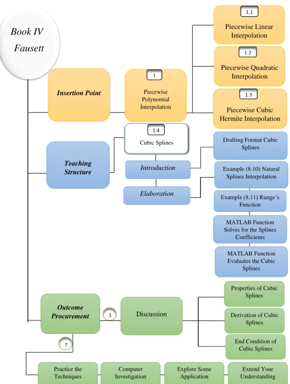
In Figure 2.26 we show a scheme of how the author presents the sectionCubic Splines in this book.

(41)

Insertion Point Properties of Cubic Splines End Condition of Cubic Splines Piecewise Cubic Hermite Interpolation Piecewise Linear Interpolation 1.1 1.3

Book IV

Fausett

Piecewise Quadratic Interpolation 1.2 Practice the Techniques Computer Investigation 1 2 Explore Some Application Extend Your Understanding Drafting Format Cubic

Splines Example (8.10) Natural Splines Interpolation Example (8.11) Runge’s Function MATLAB Function Solves for the Splines

Coefficients

MATLAB Function Evaluates the Cubic

Splines

Discussion Derivation of Cubic

Splines Piecewise Polynomial Interpolation 1 Teaching Structure Cubic Splines 1.4 Introduction Outcome Procurement Elaboration

Figure 2.26: Content and organization of Chapter 8,Interpolation, section Piecewise polyno-mial interpolation (8.3). Fausett [2008].

(42)

2.2.4.1 Insertion Point

Chapter 8 in this book is called Interpolation. In the first section of this chapter, the au-thor presents the notion of polynomial interpolation introducing Lagrange Interpolation and Newton Interpolation. In the second section Hermite interpolation is introduced. After this she demonstrates the effect of higher degree polynomial interpolation by considering Runge’s function. This example shows that increasing the degree of an interpolating polynomial does not necessarily reduce the interpolation error. Instead, high oscillations occur at the endpoints of the interval. This effect gets larger when the number of interpolation points is increased. This is the motivation for introducing piecewise polynomial interpolation in the next section. In the section Piecewise Polynomial Interpolation, the author retakes the disadvantage of high degree interpolation that has been observed in the Runge’s function. To avert the problem we can use piecewise polynomials. She motivates the section also by a reference to the historical use of splines as “the design and construction of a ship or aircraft involved the use of full-size models” [Fausett, 2008]. The author refers to the history to show why we might study how to construct a smooth curve and why. Additionally, she explains the details of how spline curves were constructed in the past. The book mentions the relation of the mathematical spline to a bent beam in physics, which takes the shape of a cubic piecewise polynomial. Then, the author presents a spline in a mathematical way by mentioning different types of piecewise polynomial interpolation of degreem. She gives a brief summary for each type of spline that will be mentioned in the next sections:

1. Linear splines, which are continuous functions.

2. Quadratic splines, which have also continuous derivatives.

3. Piecewise cubic Hermite interpolation, which “is useful [...] for shape preserving” [Fausett, 2008]. To program Hermite interpolation in MATLAB the built-in Matleb function pchipis described.

She explains the differences between nodes and knots because she distinguishes the two cases. Firstly, she treats the case “nodes=knots”, and afterwards, “nodes 6= knots”. In her definition, nodes are the points where spline segments meet and knots are the points where interpolation conditions are imposed.

Finally, after having introduced the details about the different kinds of splines, the author draws attention to cubic spline interpolation, mentioning its use in various mathematical problems. To illustrate, a plot of cubic spline interpolation vs. polynomial interpolation is given in Figure 2.27.

Piecewise Linear Interpolation

The author explains linear spline interpolation as the simplest example of piecewise interpo-lation. The explanation starts by considering a set of data points (xi, yi) and includes the details of construction of linear spline interpolation. The description is done for a set of four data points. Then she shows the formula of this spline in terms of Lagrange polynomials. In more general terms, the formula reads

(43)

Figure 2.27: Cubic spline and polynomial interpolation for Runge’s function (Fausett [2008], p.299). P(x) =                x−x2 x1−x2y1+ x−x1 x2−x1y2 x∈[x1, x2) x−xi+1 xi−xi+1yi+ x−xi xi+1−xiyi+1 x∈[xi, xi+1) x−xn xn−1−xnyn−1+ x−xn−1 xn−xn−1yn x∈[xn−1, xn] (2.12)

In addition, the author mentions the advantage that a linear spline interpolation function is continuous and the disadvantage that it has no further smoothness at the knots. Finally, she presents an example of piecewise linear interpolation of four data points Figure 2.28:

Piecewise Quadratic Interpolation

The author introduces quadratic splines by explaining the construction of a piecewise quadratic function forn+ 1 data points on nintervals. By counting the unknowns of the formula and the equation for each interval it can be seen that there are 3n−1 equations and 3nunknowns. Therefore she concludes that one additional condition is needed in order to have a solvable system. She points to several alternatives to meet this condition and presents an approach that makes it particularly easy to construct quadratic splines. The form of this spline is the following:

Si(x) =yi+zi(x−xi) +

zi+1−zi 2(xi+1−xi)

(x−xi)2, on [xi, xi+1) (2.13) wherezi is the slope atxi of the function Si(x). The author explains:

1. The continuity conditions for the first derivative at the nodes of the quadratic spline formula (2.13) are automatically enforced.

(44)

Figure 2.28: Linear piecewise interpolation of the data x = [0,1,2,3] and y = [0,1,4,3] ([Fausett, 2008, p. 300]).

2. The interpolation and continuity conditions for the quadratic spline at the knots must also be enforced.

3. The slopezi can be obtained by using continuity property of the function at the nodes. The slopes are found to satisfy

zi+1 = 2

yi+1−yi

xi+1−xi

−zi (2.14)

Thus, specifyingz1 will render the other slopes,z2, . . . , zn.

4. By giving four data points (xi, yi), i = 1,2,3,4, and computing the coefficients of the quadratic spline by using the slopes zi with the condition “nodes=knots”, the author shows that the value of the slope atx1 has considerable influence on the resulting curve. 5. Another alternative would be to choose the knots to be the midpoints of the nodes. In this case (“nodes6=knots”) we obtain six equations for eight unknowns, meaning the value for two of the slopes must be given. The author says this is a “more balanced” [Fausett, 2008] approach, as there can be end conditions at each end of the interval. The slopes zi are, in this case,

• z1 =x1 • zi = xi−1₂+xi • zn+1=xn

If the data points are spaced evenly we may definehi=xi+1−xi when i= 1, ..., n, and then

(45)

Figure 2.29: By considering the data points (0,0),(1,1),(2,4),and(3,3) and solving a linear system using MATLAB we get a piecewise quadratic interpolation function for the given data points. ([Fausett, 2008, p. 303]). • z2−x1= h₂1 • zi−xi−1= hi−₂1 • zn−xn−1 = hn−₂1 and • z2−x2= −₂h1 • zi−xi= −h₂i−1 • zn−xn= −h₂n−1

The author uses this example to illustrate the properties of quadratic splines. She points to the first property (continuity conditions at the interior nodes) of the quadratic spline function and to the second property (continuity conditions at the first derivative). A linear system with six equations and eight unknowns is obtained. The unknowns are the coefficients of the quadratic spline. Furthermore, the author demonstrates an example to evaluate the this kind of quadratic spline. Example 8.8 in the book uses the same data points as for the previous case, i.e., “nodes=knots”. Figure 2.29 shows the plot obtained for the case “nodes6=knots”. The disadvantage of using this approach is that the the matrix is not tridiagonal and thus system is more expensive to compute.

The author then turns her attention to piecewise polynomials. In the next sections better smoothness results will be obtained by Hermite interpolation and cubic spline interpolation.

Piecewise Cubic Hermite Interpolation

At the beginning of this section the author emphasizes that “one important use of Hermite interpolation is in the setting of piecewise interpolation:[it] can be used to preserve mono-tonicity” [Fausett, 2008]. It is important to explain cubic Hermite interpolation in order to understand cubic splines interpolation: a disadvantage of cubic Hermite interpolation – its low degree of smoothness – will serve as motivation for the study of cubic splines interpolation.

(46)

Figure 2.30: By considering some data point of x = [−3,−2,−1,0,1,2,3] and y = [−1,−1.1,−1,0,1,1.1,1], a) Figure 8.21: piecewise Hermite interpolation by usedpchip func-tion in MATLAB. b) Figure 8.22: polynomial interpolafunc-tion of same data ([Fausett, 2008, p.304]).

By means of a plot (Figure 2.30) using the built-in MATLAB functionpchip, the author shows that cubic Hermite piecewise interpolation polynomial has continuous first derivative at the interior nodes. The author includes in the figure a plot of polynomial interpolation of the same data in order to point out important differences between them. The polynomial interpolant is smoother but oscillates (overshoots) more.

2.2.4.2 Teaching Structure

In this section we illustrate the details of the section Cubic Spline Interpolation. In the

Introduction we will display the motivation and foundations Fausett uses to introduce this topic. Then, in theElaboration section we will study how the author develops the theory of cubic splines.

(47)

Introduction

The author starts by restating the advantage of working with cubic splines, which is to get the maximum smoothness possible. This can be calculated to be the continuity of first and second derivatives. She also points to the simplicity of calculating the required coefficients of the cubic spline after a suitable choice of basis functions.

The way this author presents this material is quite different from that of previously re-viewed books. She starts by considering the form of each spline piece:

Pi(x) =ai (xi+1−x)3 hi +ai+1 (x−xi)3 hi +bi(xi+1−x) +ci(x−xi) (2.15) wherex∈[xi, xi+1] andhi =xi+1−xi. This form is justified by observing that the second derivative of the spline will be a piecewise linear function that is continuous at the knots.

The following points are made by studying the formula (2.15): 1. The continuity condition for the second derivative is verified.

2. By using the interpolation property of the spline, Pi(xi) =yi and Pi(xi+1) =yi+1, we can calculate the coefficients bi and ci in terms of theai:

bi = yi hi −aihi ci= yi+1 hi −ai+1hi

3. By using the continuity conditions of the first derivative at the knots, with the use of the coefficientsbi,ci we get

hiai+ 2(hi+hi+1)ai+1+hi+1ai+2= yi+2−yi+1 hi+1 −yi+1−yi hi (2.16) for i= 1, ...., n−2

The author discusses how to use formula (2.16) to compute the coefficients of the cubic spline interpolant. In order to get a square system there are different choices for the required additional conditions on the second derivative at the endpoints. Then she suggests “the simplest choice” is the natural cubic spline, for which a1=an= 0.

Elaboration

By means of Example 8.10, the author illustrates the construction of a natural cubic spline interpolant. The example chooses five data points with equally spaced abscissae. She asks the reader to observe the resulting smoothness in this example and compare it to the examples for piecewise linear interpolation and piecewise quadratic spline interpolation. Figure 2.31 shows the graph of the cubic spline.

Following this example, the author describes Runge’s function in another example (Exam-ple 8.11), using the same data of Exam(Exam-ple 8.6 from the section on polynomial interpolation.

(48)

Figure 2.31: Natural cubic spline interpolating the data points (−2,4),(−1,−1),(0,2),(1,1) and (2,8) ([Fausett, 2008, p.306]).

Figure 2.32: a) [Fausett, 2008, p.292]. Figure 2.33: b) [Fausett, 2008, p.307]. Figure 2.34: a) Runge’s function and interpolation polynomial, b) Cubic spline interpolation of Runge’s function

(49)

The aims is to show a difference between the use of cubic spline interpolation and polyno-mial interpolation. One can observe in Figure 2.34 that the cubic spline does not exhibit the undesired behavior of the interpolation polynomial.

Additionally, the author gives a MATLAB code to show how to program the Runge function example by using thesplinefunction in MATLAB. After that the author shows the code of a MATLAB function for calculating the spline coefficients by using theGauss-Thomas

method for tridiagonal systems. Finally, the author presents a code for the evaluation of a cubic spline (Fausett [2008], p. 309).

In a section calledDiscussion, the author shows some theoretical aspects of the derivation of cubic splines in more detail. The author developed the following points:

1. Choice of “nodes=knots”.

2. Computation of the number of end conditions that need to added, and what formulation they can have.

3. By looking at the previous form 2.15, enforcement of the properties of thecubic splines. 4. Explanation of the steps needed to calculate the coefficients bi and ci in the previous

section.

5. Discussion of possible options for end conditions: natural cubic splines and clamped splines (which specifies the first derivatives at the endpoints).

6. Study of the error between the spline and the original function by looking at the general formula:

|S(x)−g(x)|< kh4G=(h4) (2.17)

At the end of the chapter on interpolation, the author presents a summary where the main results of polynomial interpolation, Hermite interpolation, and cubic spline interpolation are outlined. Then comes a list of suggested reading, and finally some exercises. These are divided into four sections. Practice the Techniques section has exercises to be done by hand, by interpolating with piecewise linear, piecewise quadratic and cubic splines, as well as using different bases to express the polynomials. Computer Investigationshas interpolation exercises that are to be solved using a calculator or a computer. Explore Some Applications has applied problems, some within mathematics, as statistical functions or calculation of integrals, and others outside mathematics, for instance chemical and engineering problems. The last part of this section,Extend Your Understanding, is targeted to students who wish to go a step further on the topic of Interpolation. There are some theoretical questions and some implementation issues.

(50)

(51)

Comparison and Evaluation

The intention of this chapter is to go into the details of the procedures, strategies, methods and topics that the authors have used and developed for the purpose of teaching cubic splines. In order to compare the different books, we have based our study on questions and answers. These questions have been selected to cover all the issues that need to be discussed in order to make a proper of evaluation of the material. The idea of the question-and-answer scheme is to develop the central topic of this thesis in a clear and easy manner for the reader.

Moreover, each question will have an answer for each particular book. At the end of each section we will present a table giving the details that have been discussed. The aim of these tables is to make it easy to observe the differences and similarities between these books, and to have a basis for the evaluation.

After each question is presented, we look into the facts provided by the answers and draw our own conclusions and make comparisons. Sometimes two or more books have very similar answers to a question, and other times there is a sharp contrast between books. In this section we will evaluate each book in relation to each of the posed questions.

Question 1 How is the topic of cubic splines initially

presented?

I. Steven C. Chapra’s book (Chapra [2011]).

Figure 2.3 shows the organization of the topics in the chapter Splines and Piecewise Interpolation. Where the subject of cubic splines is introduced and explained. A plan of the chapter is displayed in Figure 2.3.

As observed in Figure 2.3 the insertion point rests on three introductory sections. Firstly, Introduction to Splines, the main thrust of this section is to show a difference between different kinds of interpolation splines by increasing data points, and giving a simple example and showing Figure 2.7 to make the idea clear.

Additionally there is a brief summary, looking into its historical development. Secondly, linear splines are explained in precise details. An introduction to linear splines includes an example to explain the formula and how one can calculate the linear splines that interpolate some data. Moreover, the book mentions that data points can be interpo-lated by splines of different orders. Furthermore, advantages and disadvantages of linear