A Simulated Data Analysis on the Interval Estimation for the Binomial Proportion P

A Simulated Data Analysis on the Interval Estimation for the

Binomial Proportion

P

Junge B. Guillena

Adventist Medical Center College, Iligan City, Philippines

[email protected]

Abstract

This study constructed a quadratic-based interval estimator for binomial proportion p. The modified

method imposed a continuity correction over the confidence interval. This modified quadratic-based

interval was compared to the different existing alternative intervals through numerical analysis using the

following criteria: coverage probability, and expected width for various values of n, p and α = 0.05.

Simulated data results generated the following observations: (1) the coverage probability of modified

interval is larger compared to that of the standard and non-modified intervals, for any p and n; (2) the

coverage probability of all the alternative methods approaches to the nominal 95% confidence level as n

increases for any p;(3) the modified and non-modified intervals have indistinguishable width differences

for any p as n gets larger; (4) the expected width of the modified and alternative intervals decreases as n

increases for





0

.

05

and any p. Based on these observations one can say that the modified method is

an improvement of the standard method. It is therefore recommended to modify other existing alternative

methods in such a way that there’s an increase in performance in terms of coverage properties, expected

width, and other measures.

Keywords:

Confidence Interval, Binomial Distribution, Standard Interval, Coverage Probability,

Expected Width

Introduction

Inferential problem like interval estimation arising from binomial experiments is one of the classical problems in statistics offering many arguments and disputes. When constructing a confidence interval, one usually wishes the actual coverage probability to be close to the nominal confidence level, that is, it closely approximates to

1





. The unexpected difficulties inherent to the choice of a confidence interval estimate of the binomial parameter p, and the relative inefficiency (Marchand, E., Perron, F., and Rokhaya, G., 2004) f the “standard” Wald confidence interval, has resurfaced recently with the work of Brown, L. D., Cai, T.T., and DasGupta, A. (1999a and 199b) and Agresti and Coull (1998). Along with this, several alternative interval estimates have been suggested. Some alternative intervals make use of a continuity correction while others guarantee a minimum

1





coverage probability for all values of the parameter p. In line with this, this study aims to develop an alternative method with slight modifications of the method first developed by Casella, et al., 1990. As suggested, this modification imposes a continuity correction factor.

Purpose of the Study

The objective of this study is to construct a non-randomized confidence interval

C

 

X

for p, such that the coverage probability

P

_p



p



C

 

x





1





, where



is some pre-specified value between 0 and 1 (Casella and Berger, 1990) Specifically, the objective of this study is to compare numerically the performance of the standard, non-modified and non-modified intervals and some alternative interval estimators based on coverage probability and expected width.

BASIC CONCEPTS:

Confidence Interval

Definition 1: Let

X

₁

,

X

₂

,...

X

_n be a random sample from the density

f

 

x



. Let

l

(

x

)



l



x

₁

,

x

₂

,...

x

_n



and



x

x

x

n



u

x

u

(

)



1

,

2

,...

be two statistics satisfying

l

   

x



u

x

for which

P





l

(

x

)







u

(

x

)





1





. Then the random interval



l

(

x

),

u

(

x

)



is called a

100

(

1





)%

confidence interval for



;

1





is called the confidence coefficient; and

l

(

x

)

and

u

(

x

)

are called the lower and upper confidence limits, respectively, for



.

Expected Width and Coverage Probability: Some criteria for evaluating interval estimators are the interval width and coverage probability. Ideally, an interval must have narrow width with large coverage probability, but such sets are usually difficult to construct.

Definition 2: The coverage probability of the confidence set

C

 

x

is defined as

 











_

_







 

 







C

X

I

C

x

dF

x

P

where:



is the sample space of X and

I







C

(

x

)



is an indicator function for a nonrandomized set equal to 1 if

 

x

C





, otherwise it is 0.

Definition 3: The expected width is defined as:

 







   



 





width

of

C

X

U

X

L

X

f

x

E

n x n









0 , , where

 

X

U

and

L

 

X

are the upper and lower limits respectively of the confidence set

C

 

x

Standard Interval Estimator: A standard confidence interval for p based on normal approximation has gained universal recommendation in the introductory statistics textbooks and in statistical practice. The interval is known to guarantee that for any fixed p, the coverage probability

P



p



C

 

x





1





as

n





.

To show this interval estimator, let



 

z

and



 

z

be the standard normal density function and cumulative distribution, respectively. Let



2





1



1





2





z

z

,

n

x

p

ˆ



and

q

ˆ



1



p

ˆ

, where

p

ˆ



q

ˆ



1

.The normal



ˆ



The Proposed Modified Interval: Due to the discreteness of the binomial distribution and as suggested by Casella, et al., 1990, this proposed modified interval imposes a continuity correction,

n

c

4

1



, over the modified interval. The factor is arbitrarily chosen.

Theorem 1: The approximate

1





confidence interval for p with

n

c

4

1



is given by

 

































































_















































n

z

n

z

n

p

n

z

n

p

n

z

n

p

X

C

2 2 2 1 2 2 2 2 2 2 2

1

2

1

4

1

ˆ

4

2

1

ˆ

2

2

1

ˆ

2

   

where the lower limit is given by,

 

































































_















































n

z

n

z

n

p

n

z

n

p

n

z

n

p

n

x

L

2 2 2 1 2 2 2 2 2 2 2

1

2

1

4

1

ˆ

4

2

1

ˆ

2

2

1

ˆ

2

,

   

and upper limit is given by

 

































































_















































n

z

n

z

n

p

n

z

n

p

n

z

n

p

n

x

U

2 2 2 1 2 2 2 2 2 2 2

1

2

1

4

1

ˆ

4

2

1

ˆ

2

2

1

ˆ

2

,

   

Simulated Results and Discussions: This section presents the comparative graphical and numerical results and comparisons of the different alternative interval estimators, in terms of its coverage probability behavior, and expected width. In investigating the performance of the standard interval and the alternative intervals, the usual



= 0.05 is utilized. Simulation of data values was done through Maple program.

Comparison for Standard, Non-Modified and Modified Intervals in terms of Coverage Probability:

Figures 1 presents the result of the coverage graphs of the standard, the non-modified and the modified intervals for

n = 20, 40, 70 and 100 with nominal 95%. It shows that both the non-modified and the standard intervals have significantly downward spikes near p close to 0 or 1, while the modified interval has a good coverage probability behavior for any p. The above aforementioned results give evidences and supports to the following claim: the coverage probability of the modified interval has much better behavior over the standard and the non-modified intervals for any p and n.

Comparison for Modified and Alternative Intervals

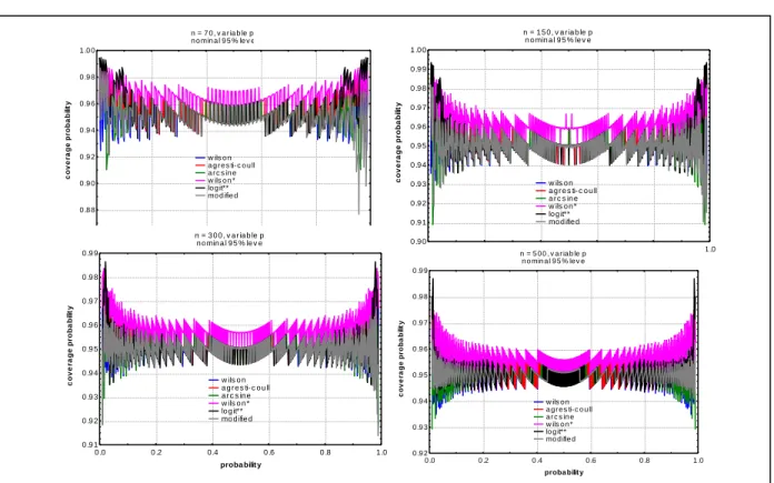
Figures 2 shows the result of the coverage probability graphs of the Wilson, the Agresti – Coull, the arcsine, the Wilson*, the Logit**, and the modified intervals for n = 70, 150, 300 and 500 with variable p for nominal 95% confidence level. It reveals that the Agresti-Coull interval has conservative coverage probability near p = 0, which means that most of the coverage probability is above the nominal level. On the other hand, the Wilson interval has a fairly downward spike near 0 or 1, but has a good coverage probability away from the boundaries. The arcsine interval has an erratic pattern near the boundaries, since the coverage probability cuts off quickly at some values of



0

.

034

,

0

.

054





p

or

p





0

.

946

,

0

.

966



with values below 0.95. The modified interval has some downward spike near the boundaries but gradually disappear as p approaches to 0.5 or away from 0 or 1. This interval is comparable to other alternative intervals like the logit**, the Wilson, the arcsine but less comparable to the Agresti-Coull and Wilson* intervals in terms of coverage probability behavior. When

p





0

.

01

,

0

.

086



or



0

.

914

,

0

.

99





p

the Agresti-Coull interval aside from the Wilson* have coverage probabilities greater than 0.95. For larger values of n, which in this case n = 300 and 500, the Wilson* has a consistent coverage probability behavior that is greater than or equal to 0.95 for all values of p. The Wilson, arcsine, logit** and modified intervals have some downward spike near p = 0.01, but still the coverage probability of these intervals perform well in the middle parameter space region. These numerical findings show that the modified interval has a comparable coverage probability behavior both in n = 70, 150, 300 and 500 for nominal 95% confidence level. These results give support to the following suggestion that the coverage probability behavior of all the methods approaches to the nominal 95% confidence level as n increases for any p.

n = 20, variable p nominal 95% level 0.0 0.2 0.4 0.6 0.8 1.0 p r o b a b ility 0.1 0.2 0.3 0.4 0.5 0.6 0.7 0.8 0.9 1.0 c o v e ra g e p ro b a b ili ty standard nonmodified modified n = 40, variable p nominal 95% level 0.0 0.2 0.4 0.6 0.8 1.0 proba bilit y 0.2 0.3 0.4 0.5 0.6 0.7 0.8 0.9 1.0 c o v e ra g e p ro b a b ili ty standard non-modified modified n = 70, variable p nominal 95% level 0.0 0.2 0.4 0.6 0.8 1.0 proba bilit y 0.4 0.5 0.6 0.7 0.8 0.9 1.0 c o v e ra g e p ro b a b ili ty standard non-modified modified

Figure 1

Comparison of coverage probability of the standard, the non-modified and

the modified intervals for

n

= 20, 40, 70 and 100 with

1







0

.

95

n = 100, variable p nominal 95% level 0.0 0.2 0.4 0.6 0.8 1.0 proba bilit y 0.50 0.55 0.60 0.65 0.70 0.75 0.80 0.85 0.90 0.95 1.00 c o v e ra g e p ro b a b ili ty standard non-modified modified

Comparison for Standard, Non-Modified and Modified Intervals in terms of Expected Width

Figure 3 shows the comparison of expected width of the standard, the non-modified and the modified intervals for n

= 20, 40, 70 and 100 with nominal 95% level. Results show that at smaller (

n



40

), the modified interval has larger width near the boundaries 0 or 1, but as p approaches to 0.5, it has similar width with the non-modified interval. The standard interval has wider width near p close to 0.5. But as n increases, they have comparable width performance. The preceding results give validity to the conjecture that the non-modified and the modified intervals have comparable expected width when n gets larger for any p.

n = 7 0 , v a r ia b le p n o min a l 9 5 % le v e l 0 .0 0 .2 0 .4 0 .6 0 .8 1 .0 proba bilit y 0 .8 6 0 .8 8 0 .9 0 0 .9 2 0 .9 4 0 .9 6 0 .9 8 1 .0 0 c o v e ra g e p ro b a b ili ty w ils o n a g r e s ti- c o u ll a r c s in e w ils o n * lo g it** mo d ifie d

Figure 2 Comparison of coverage probability of the Wilson, the Agresti-Coull, the arcsine, the Wilson*, the logit** and the modified intervals for n = 70, 150, 300 and 500 with

1







0

.

95

.

n = 1 5 0 , v a r ia b le p n o min a l 9 5 % le v e l 0 .0 0 .2 0 .4 0 .6 0 .8 1 .0 proba bilit y 0 .9 0 0 .9 1 0 .9 2 0 .9 3 0 .9 4 0 .9 5 0 .9 6 0 .9 7 0 .9 8 0 .9 9 1 .0 0 c o v e ra g e p ro b a b ili ty w ils o n a g r e s ti- c o u ll a r c s in e w ils o n * lo g it** mo d ifie d n = 3 0 0 , v a r ia b le p n o min a l 9 5 % le v e l 0 .0 0 .2 0 .4 0 .6 0 .8 1 .0 proba bilit y 0 .9 1 0 .9 2 0 .9 3 0 .9 4 0 .9 5 0 .9 6 0 .9 7 0 .9 8 0 .9 9 c o v e ra g e p ro b a b ili ty w ils o n a g r e s ti- c o u ll a r c s in e w ils o n * lo g it** mo d ifie d n = 5 0 0 , v a r ia b le p n o min a l 9 5 % le v e l 0 .0 0 .2 0 .4 0 .6 0 .8 1 .0 proba bilit y 0 .9 2 0 .9 3 0 .9 4 0 .9 5 0 .9 6 0 .9 7 0 .9 8 0 .9 9 c o v e ra g e p ro b a b ili ty w ils o n a g r e s ti- c o u ll a r c s in e w ils o n * lo g it** mo d ifie d

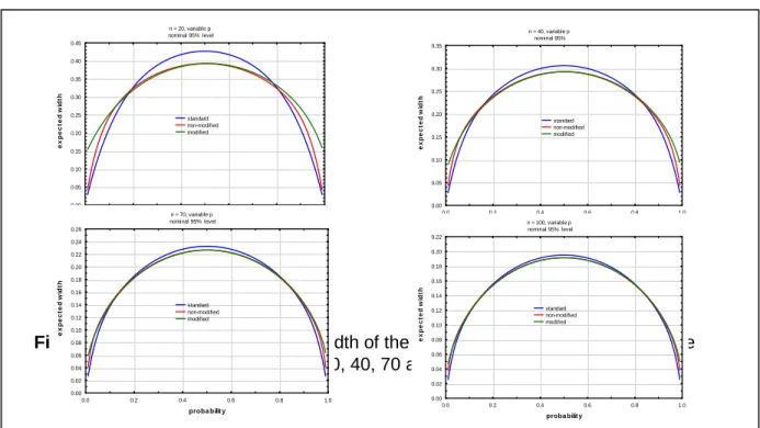
Comparison for Modified and Alternative Intervals in terms of Expected Width

Figure 4 displays the result for the graphs of the expected width of the Wilson interval, the Agresti-Coull interval, the arcsine interval, the Wilson*, the logit** interval and the modified interval for n = 40, 80, 150 and 300 with nominal 95% confidence level, respectively. Result shows that the modified interval has the shortest width when

0

.

139



p



0

.

861

, the Wilson interval and Agresti-Coull interval have a comparable width with the modified interval when p approaches 0.5, the Wilson* interval is consistent for having the largest width when

104

.

0



p

or

p



0

.

896

, and the logit** interval is the largest at near the boundaries or when

p



0

.

103

. These numerical evaluations show that the modified interval has a better performance in terms of expected width, the Wilson* has a larger width of what is expected since this interval is partly conservative in terms of coverage properties especially near the boundaries. For n = 150, the standard interval shows the shortest when

114

.

0



p

or

p



0

.

886

; the modified interval is the shortest when

p



0

.

115

or

p



0

.

885

, and still the Wilson (0.5) is the largest for most values of n, and the logit** interval is the largest when p nearer the boundaries. For n = 300, the results show that the standard interval is the shortest when

p



0

.

102

or

p



0

.

898

, the Wilson, Agresti-Coull, arcsine, logit** and modified intervals have almost indistinguishable width difference when

103

.

0



p

or

p



0

.

887

, while the Wilson* is significantly larger. This suggests that the Wilson, Agresti-Coull, arcsine, Logit (-0.87) and the modified intervals are all preferable methods for larger values of n in terms of expected width. But if the precision of the estimate is preferred for an increased width, Wilson (0.5) interval is preferable especially for larger values of n. The aforementioned results build up the following evidence that the interval that has a coverage probability closely approximate to the nominal 95% confidence level, yields a narrower expected width.

Figure 3

Comparison of Expected Width of the standard, the non-modified and the

modified intervals for

n

= 20, 40, 70 and 100 with

1







0

.

95

n = 20, variable p nominal 95% level 0.0 0.2 0.4 0.6 0.8 1.0 proba bilit y 0.00 0.05 0.10 0.15 0.20 0.25 0.30 0.35 0.40 0.45 e x p e c te d w id th standard non-modified modified n = 40, variable p nominal 95% 0.0 0.2 0.4 0.6 0.8 1.0 proba bilit y 0.00 0.05 0.10 0.15 0.20 0.25 0.30 0.35 e x p e c te d w id th standard non-modified modified n = 70, variable p nominal 95% level 0.0 0.2 0.4 0.6 0.8 1.0 proba bilit y 0.00 0.02 0.04 0.06 0.08 0.10 0.12 0.14 0.16 0.18 0.20 0.22 0.24 0.26 e x p e c te d w id th standard non-modified modified n = 100, variable p nominal 95% level 0.0 0.2 0.4 0.6 0.8 1.0 proba bilit y 0.00 0.02 0.04 0.06 0.08 0.10 0.12 0.14 0.16 0.18 0.20 0.22 e x p e c te d w id th standard non-modified modified

Conclusion and Recommendation

The existing and additional results would suggest rejection of the conditions made by several authors regarding the use of the standard interval, but instead utilize the alternative methods found in the literature which perform better in terms of coverage properties and other criteria. The performance of the alternative methods and the proposed method modified by the researcher and the results show that some of these intervals have very good coverage probability behavior and smaller expected width.

Given the varied options, the best solution will no doubt be influenced by the user’s personal preferences. A wise choice could be either one of the Wilson, Agresti-Coull, Wilson*, logit**, arcsine and modified intervals which show decisive improvement over the standard interval. Based on the analysis and results obtained, the researcher’s recommendations to compare and investigate the performance (like coverage properties) of the most probable classical and Bayesian intervals and examine the RMSE property of the modified interval discussed in the current study.

References

Agresti, A., and Caffo, B. (2000). Simple and Effective Confidence Intervals for Proportions and Differences of Proportions Result from Adding Two Success and Two Failures. The American Statistician, 54, 280 – 288

.

Boomsma, A. (2005). Confidence Intervals for a Binomial Proportion. University of Groningen. Department of

n = 40, variable p nominal 95% level 0.0 0.2 0.4 0.6 0.8 1.0 proba bilit y 0.06 0.08 0.10 0.12 0.14 0.16 0.18 0.20 0.22 0.24 0.26 0.28 0.30 0.32 0.34 e x p e c te d w id th wilson agresti-coull arcsine wilson* logit* * modified n = 80, variable p nominal 95% level 0.0 0.2 0.4 0.6 0.8 1.0 proba bilit y 0.02 0.04 0.06 0.08 0.10 0.12 0.14 0.16 0.18 0.20 0.22 0.24 e x p e c te d w id th wilson agresti-coull arcsine wilson* logit* * modified n = 150, variable p nominal 95% level 0.0 0.2 0.4 0.6 0.8 1.0 proba bilit y 0.02 0.04 0.06 0.08 0.10 0.12 0.14 0.16 0.18 e x p e c te d w id th wilson agresti-coull arcsine wilson* logit* * modified n = 300, variable p nominal 95% level 0.0 0.2 0.4 0.6 0.8 1.0 proba bilit y 0.00 0.02 0.04 0.06 0.08 0.10 0.12 e x p e c te d w id th wilson agresti-coull arcsine wilson* logit* * modified

Figure 4 Comparison of expected width of the Wilson, the Agresti-Coull, the arcsine, the Wilson*, the logit** and the modified intervals for n = 40, 80, 150 and 300 with

1







0

.

95

.

Brown, L. D., Cai, T. T., and DasGupta, A. (1999a). Interval Estimation of a Binomial Proportion. Unpublished Technical Report

Brown, L. D., Cai, T. T., and DasGupta A. (1999b). Confidence Intervals for a Binomial Proportion and Edgeworth Expansion. Unpublished Technical Report.

Brown, L. D., Cai, T. T., and DasGupta A. (2001). Interval Estimation for a Binomial Proportion (with discussion).

Statistical Science, 16, 101 – 133.

Brown, L. D., Cai, T. T., and DasGupta A. (2002). Confidence Intervals for a Binomial Proportion and Asymptotic Expansions. The Annals of Statistics, 30, 160 – 201.

Casella, G., and Berger, R. (1990). Statistical Inference. Pacific Coast, CA. Woodsworth and Brooks/Cole.

Dippon, J. (2002). Moment and Cumulants in Stochastic Approximation. Mathematisches Institut A, Universitat Stuttgart, Germany.

Edwardes, M. D. (1998). The Evaluation of Confidence Sets with Application to Binomial Intervals. Statistica Sinica, 8, 393 – 409.

Harte, D., (2002). Non Asymptotic Binomial Confidence Intervals. Statistics Research Associates, PO Box 12 649, Wellington NZ.

Marchand, E., Perron, F. & Rokhaya, G., (2004). Minimax Esimation of a Binomial Proportion p when [p – ½] is bounded. Universite’ de Montreal