Shared Control of Mobile Robots Using Model Predictive Control

SHARED CONTROL OF MOBILE ROBOTS

USING MODEL PREDICTIVE CONTROL

Master of Science Thesis Faculty of Engineering and Natural Sciences Examiners: Associate Professor Reza Ghabcheloo Associate Professor Roel Pieters October 2020

Tarun Reddy Devalla: Shared Control of Mobile Robots using Model Predictive Control Master of Science Thesis

Tampere University

Automation Engineering, Factory Automation and Robotics October 2020

With the world constantly driving towards attaining complete autonomy, there is still a ma-jor question of safety when it comes to trusting a machine completely. Autonomous systems of today also do not have the ability to perform flawlessly in an environment that is cluttered and unstructured. This calls for the need of having a human operate the machine at all times ei-ther remotely via tele-operation methods or by being physically present alongside the machine. With tele-operation of remote systems, the cognitive load required from the human operator is high, while also the perception of the remote systems environment is low. This can cause many undesirable human errors causing damage to machinery. For example, tele-operating a forestry machine in a forest can be a very daunting task as there will be many trees and not all trees around the machine can be seen by the operator during remote tele-operation. With this in context, a few industries and sectors have now largely started research with using shared control methodologies to aid their machine in tele-operation tasks.

This thesis proposes a shared control methodology to provide a certain level of autonomy to the machine while still allowing the human operator to always be in control. The proposed methodology uses a Model predictive controller as the base controller to control the robot and perform obstacle avoidance tasks. The robot considered for implementation is a differential drive mobile robot, in specific the MiR 100 from Mobile Industrial Robots. The key motivation behind the thesis is to evaluate the performance of the shared control approach against a manual tele-operation task, to better understand the advantages and possible disadvantages of using a shared control strategy. The proposed strategy is implemented using the CasADi optimization toolbox on Matlab and tested through user testings. The results obtained from the user test prove that shared control can largely help in improving the safety of the system, but not so much with performance, at least not with the proposed methodology.

Keywords: Shared Control, Mixed Control, Human-Robot Interaction, HRI, Human in the Loop, Mobile Robot, Differential drive robot, Model Predictive Control, MPC, Receding Horizon Control, Obstacle Avoidance, teleoperation

PREFACE

This thesis is written as a part of the completion for my Master’s Degree Program in Automation Engineering at Tampere University, under the department of Engineering and Natural Sciences. I would like to thank my thesis supervisor Prof. Reza Ghabcheloo for his mentoring and guidance throughout the thesis process, and for showing persistent faith in my capabilities. His trust has been a key motivation for accomplishing my masters degree. I would also like to extend my gratitude to my thesis examiner Prof. Roel Pieters for his valuable inputs and feedback. I thank all my fellow colleagues and peers for their support and advice during the course of my master’s program.

I want to express my gratitude towards my parents, sisters and grand parents by dedi-cating this work to them. It is their unconditional support in all my decisions which has helped me in achieving my aspiration so far.

Finally, the note of thanks cannot end without mentioning my dear friends. They have been a significant part in molding me personally and in my career aspirations. On a special note, I would like to extend my gratitude to Pinaki Halale for her constant moral and emotional support towards the final phase of my thesis.

Tampere, 25th October 2020

1 Introduction . . . 1 1.1 Motivation . . . 2 1.2 Research Questions . . . 3 1.3 Objectives . . . 3 1.4 Thesis Structure . . . 4 2 Literature Review . . . 5

2.1 Shared Control: Intention and Arbitration . . . 5

2.1.1 Virtual Fixtures . . . 5

2.1.2 Mode Switching . . . 9

2.1.3 Sliding Autonomy . . . 9

2.1.4 Policy Blended/Probabilistic Approaches . . . 10

2.2 Shared Control: Communication . . . 12

2.3 A Brief Summary of Shared Control Methodologies . . . 13

2.4 Model Predictive Control . . . 14

3 Methodology and implementation . . . 17

3.1 Shared Control Methodology . . . 17

3.1.1 Kinematic Modeling of a Differential Drive Mobile Robot . . . 18

3.1.2 Model Predictive Control formulation . . . 21

3.1.3 Modelling Obstacles as Constraints . . . 24

3.1.4 Inclusion of Human Inputs into the system . . . 30

3.2 Shared Control Implementation . . . 33

3.2.1 The Simulation Environment . . . 33

3.2.2 Completing the Pipeline for Shared Control Implementation . . . . 35

4 User testing and results . . . 41

4.1 Test Procedure . . . 41

4.1.1 Manual tele-operation . . . 41

4.1.2 The user testing tasks . . . 42

4.2 Test setup . . . 42

4.3 Results . . . 44

4.3.1 Task 1 - How safe can you manoeuvre? . . . 45

4.3.2 Task 2 - How quick can you manoeuvre? . . . 46

5 Analysis . . . 48

5.1 Shortcomings . . . 48

6 Conclusions . . . 52

6.1 Future Scope . . . 53

References . . . 54

Appendix A Models . . . 58

A.1 The modified MiR Description File . . . 58

A.2 The camera description file . . . 66

Appendix B Codes . . . 68

B.1 Matlab MPC Code - no obstacle Matlab simulation . . . 68

B.2 Matlab MPC Code - obstacle avoidance Matlab simulation . . . 72

B.3 Matlab MPC code - MiR Shared Control . . . 77

B.4 Code for human joystick inputs . . . 83

B.5 Code for updating pose of user controlled point . . . 85

B.6 Code for direct tele/operation of the robot . . . 88

Appendix C User Tests of Shared Control Implementation . . . 91

C.1 Consent Form . . . 92

1.1 A generalised representation of a Shared Control System. . . 2

2.1 (a) GVF assisting a robot to follow a path (dotted line), (b) FRVF preventing robots from entering a forbidden region(grey shaded region) [3]. . . 7

2.2 Types of virtual guides [44]. . . 8

2.3 A representation of sliding dial approach for balancing workload between operator and autonomous system [28]. . . 10

2.4 Control Flow of a Policy Blended Shared Control Structure [9]. . . 11

2.5 Estimation of goal probabilities and value function with effect of human input on the system [15]. . . 12

2.6 Model Predictive Control Strategy [7] . . . 14

2.7 The system model presented in [40] for an MPC based shared control approach. . . 15

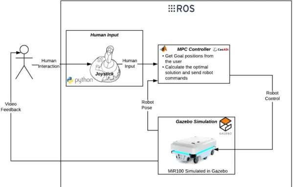
3.1 Schematic view of the implemented shared control architecture with the different software/tools used at each block. . . 17

3.2 MiR 100 Mobile Robot [27] . . . 18

3.3 2D representation of the MiR100 . . . 19

3.4 Illustration of velocity vector

v

decomposition . . . 20

3.5 (a) An example point stabilization problem with a constant goal pose

x

_g

=

[︂

x

_ref

y

_ref

θ

_ref

]︂

, (b) An example trajectory tracking problem with a goal pose

x

_g

(

t

) =

[︂

x

_ref

(

t

)

y

_ref

(

t

)

θ

_ref

(

t

)

]︂

changing with respect time

t

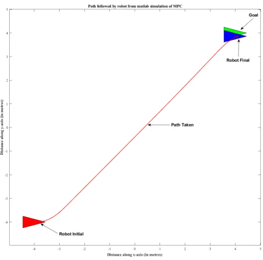
. . . 22

3.6 Visualization of the Robot path followed using the MPC algorithm in an environment without obstacle. . . 25

3.7 Plot of the control values generated by the MPC for the path in the figure 3.6 25 3.8 Representation of the static obstacles in the simulation environment. . . . 27

3.9 An example representation of obstacle avoidance modelling with a single obstacle. . . 28

3.10 Visualization of the Robot path followed using the MPC algorithm in an environment without obstacle. . . 30

3.11 Plot of the control values generated by the MPC for the path in the figure 3.6 31 3.12 A representation of the control point controlled by the human at a distance

d

_{P R}in front of the robot. . . 32

3.13 Pipeline illustrating AirSim’s modules and communication between them. . 34 3.14 General structure of the Gazebo simulation environment components [19]. 34 3.15 The modified MiR robot with cameras. . . 35 3.16 The Gazebo simulation environment created for testing the shared control

approach. . . 36 3.17 Sequence Diagram of the Different modules and their communications. . . 37 3.18 Visualization of the Robot path followed using the Shared Control

algo-rithm in the gazebo environment. . . 39 3.19 Plot of the control values generated by the MPC for the path in the figure

3.18. . . 39

4.1 Front camera feed of the robot used as a display for the user testing. . . . 43 4.2 Rear camera feed of the robot used as a display for the user testing. . . . 43 4.3 (a) A view of the user controlled pose on the environment for the

imple-mented Shared Control Approach. (b) A representation of the pose of the user controlled point with respect to the robot provided as an additional visual aid for the users. . . 44 4.4 The complete user test setup at Tampere University, Hervanta Campus. . 45 4.5 Task 1(a) A plot depicting the average number of collisions occurred in

2 minutes using manual tele-operation and shared control. (b) Plot show-ing the number of collisions per user for the 2 minutes that the task was performed. . . 46 4.6 Task 2(a) A plot depicting the average time taken to complete the given

task using manual tele-operation and shared control with and without a training period. (b) Plot showing the time taken per user for task com-pletion using manual tele-operation and shared control with and without a training period. . . 47

5.1 Plot depicting the time taken for task completion by the best driver and worst driver . . . 49

2.1 The LOA taxonomy for dynamic systems [12, 16] . . . 6

3.1 Parameters and error of the controller in an environment without obstacles. 26 3.2 Parameters and error of the controller with obstacles included. . . 29

LIST OF PROGRAMS AND ALGORITHMS

3.1 Model Predictive Algorithm. . . 26 3.2 Shared Control Algorithm . . . 38 A.1 The modified MiR description file to include cameras. . . 58 A.2 Camera definition URDF file used by the modified MiR description file. . . 66 B.1 Matlab script for MPC adapted from [43] . . . 68 B.2 Matlab script for MPC obstacle avoidance adapted from [43] . . . 72 B.3 Matlab script for MPC based Shared Control through ROS. . . 77 B.4 Script for subscribing joystick commands and publishing as twist commands. 84 B.5 Script for subscribing Twist commands from the joystick node and

publish-ing the updated pose of human controlled point. . . 85 B.6 Ros python script used for direct tele-operation of the MiR in the simulation

2D 2-Dimensional 3D 3-Dimensional

CTRM Contextual Task Recognition Module DOF Degrees of Freedom

d

_RO Distance between the robot and the obstacle e.g. Exempli gratia (For example Latin abbreviation) Et al. et alia

FRVF Forbidden Region Virtual Fixture GMM Gaussian Mixture Model

GMR Gaussian Mixture Regression GVF Guidance Virtual Fixture

J

Cost/Objective function MPC controller k Current time step in discrete time

LATEX a document preparation system for scientific writing LOA Levels of Autonomy

MCAM Motion Command Arbitration Module MDP Markov Decision Process

MiR Mobile industrial Robots MPC Model Predictive Control

N

_O Total number of obstacles

N

Prediction Horizon for the MPC controller POMDP Partially Observable Markov Decision Process

Q

3X3 Positive definite diagonal weighting matrix for the States QMDP Q-learning Markov Decision Process

R

2X2 Positive definite diagonal weighting matrix for the control inputs RBF Recursive Bayesian filter

r

_R Radius of the robot TAU Tampere University

θ

_R Robot heading

θ

̇

Rate of angular change of the robot

θ

_ref Goal heading

θ

_P Heading of Human controlled Point TUNI Tampere Universities

u

Control variables for the MPC controller URL Uniform Resource Locator

v

_acc Limit on the increase of linear velocity

v

_dec Limit on the decrease of linear velocity

v

Linear velocity

w

_acc Limit on the increase of angular velocity

w

_dec Limit on the decrease of angular velocity

w

Angular velocity

x

Robot State

x

̇

Velocity component along x axis

x

g Goal state

x

_ref X axis position of Robot goal

x

_P Pose of human controlled point

x

_P X axis position of Human controlled Point

p

_obs Obstacle position

x

_obs X axis position of obstacle

x

_R X axis position of Robot

y

̇

Velocity component along y axis

y

_ref Y axis position of Robot goal

y

_P Y axis position of Human controlled Point

y

_obs Y axis position of obstacle

1 INTRODUCTION

Today autonomous systems are peaking interests in quite many fields, with many dis-ciplines seeking out autonomous solutions for automating processes thereby reducing human labour. This approach might be pretty straight forward and an achievable dream for fixed tasks in well-defined environments. But, when we take into consideration com-pletely unstructured environments with dynamic changes, automated systems are still not preferred. The drawbacks of today are not restricted just to the environmental factors, but, also due to high complexity of some machinery that can make it difficult for complete automation. Tele-operation of such machines will also require highly skilled and trained operators [13].

There has been a rise in autonomous systems being deployed in various fields such as defense, aviation and automobile without having high predictability of the environment and a system where failure is completely acceptable [2]. At times such as this, humans are in complete control of the vehicle either on the machine or through tele-operation as they have the capability to perceive the environmental conditions well enough to control the machine. Even so this poses a few problems with tele-operation like, limited situational awareness of the environment and communications delays. This can lead to unexpected collisions in the environment and damage to the machinery [40].

Tele-operation can be a task that requires high cognitive abilities from the human operator demanding high levels of alertness at all times. This can become a very demanding job especially in environment with many dynamically moving objects. Tasks like search and rescue operations, require a human to be in control of the machine always, like in using tethered underwater rescue robots which is just one example. The tele-operation of the machine can prove to be a rather daunting task without the right system design and providing a high situational awareness to the user [29].

With more data being transferred to the user, to provide a good feel of the real system, the delays within the system can start drastically increasing as well. The user will, however, not have complete feel of driving a real machine and can become very comfortable with controlling the system at full throttle. When in fact, the system may at times not behave as expected, causing an undesired movement of the robot.

Figure 1.1. A generalised representation of a Shared Control System.

1.1 Motivation

Shared control can be seen as a solution bridging the gap between completely au-tonomous systems and completely manual systems by introducing an architecture that has the human always in the loop, while also giving certain level of autonomy to the ma-chine. This might now raise another question, what is shared control? Till date, shared control does not have an outright definition. A shared control system can simply be recog-nised as any system within which task execution collectively depends on both the human input and input from an autonomous controller on the machine.

A generalised representation of a shared control system can be seen in Figure 1.1. The controller, takes as input, the desired control inputs from the human operator, the inputs calculated by the robot’s on-board PC and the robot’s current state. It uses these to calculate a desirable control value for moving/manipulating the robot. The controller can also give haptic force feedback to the operator to increase the operators perception on the task execution. The system may also have additional aids for the human to increase perception. For example, a video feed or visualization of the sensor data.

Shared control systems are by large increasing in popularity off late with 5% increase in year-by-year number of publications. There has also been a diversification to the different applications where shared control has been used, which include:

1. Automotive industry

2. Drone control and navigation 3. Robotic surgery

4. Brain Machine Interfaces (BMI) for prosthetic and wheelchair control 5. Mobile robots control and navigation

These are just a few of the prominent application areas where shared control is currently in use [2]. But on a closer look, we can conclude that most of these tasks still require the

This brings systems with shared control strategies into play, to enable more dynamic and safe tele-operation of mobile machines and remote robotic systems. Shared control can be implemented in various different methods as the concept is rather very broad. A few different methodologies will be discussed later in the next chapter to give a good idea of how a shared control approach can be adopted for the task at hand.

1.2 Research Questions

As mentioned above, shared control can be used for various applications. But to evaluate a shared control architecture, a few questions need to be tended to.

1. How to include Human in the Loop control for shared control?

2. How can having a shared control approach help with more efficient robot control in terms of maneuverability?

3. Can the use of a shared control approach help with increasing the safety of robot during tele-operation?

1.3 Objectives

The key objective of the thesis is, to develop a shared control architecture to enable a human-in-the-loop control scheme using a 3D simulation environment and a mobile robot. A mobile robot can be either a small indoor mobile robot, like the MiR100 or a much larger mobile machine, like a hydraulic wheel loader. For this thesis we use a non-holonomic mobile robot, MiR 100, to test the implementation. But, the method should be portable to any mobile machine using the appropriate system model.

To do so a suitable test environment needs to created to test the shared control system that will be implemented. The main robot controller will be controlled using Model Pre-dictive Control (MPC) approach and the user will provide inputs to the system using a joystick of 2 DOF, as the current robot has only 2 controllable Degree of Freedom. After implementation of the shared control architecture, the system is to be tested with users of different skill level and technical backgrounds to achieve an unbiased analysis of the system.

1.4 Thesis Structure

The document has a total of 6 chapters, with the first being the introduction of the thesis, giving an idea to shared control systems and scope of this thesis.

Chapter 2 gives a theoretical background to the different shared control implementations, along with a short literature review on MPC approaches.

Chapter 3 presents the thesis methodology and implementation which will include the kinematic modelling of the mobile robot, the MPC formulation, introduction to the simula-tion environment and the proposed shared control architecture.

Chapter 4 focuses on presenting the approach taken for performing the user tests of the implemented shared control methodology mentioned in chapter 3. This chapter also provides the results from the user testing and along with a comparison of performance between a shared control approach against a conventional tele-operation approach.

Chapter 5 provides a comprehensive analysis based on the results from user testing highlighting the shortcomings of the implemented shared control architecture.

Finally, Chapter 6 concludes the works of this thesis, along with future works to further enhance and develop the research on this topic.

2 LITERATURE REVIEW

As discussed in chapter 1 shared control doesn’t have a discrete definition and this can make this a rather widespread topic with various different applications and implementa-tions to it. To grasp a clear and concise understanding of the topic, a comprehensive literature study of some of the methodologies will be presented below. Shared control in a generalised format can be seen as a collective implementation of the following three parts [24]:

1. Intent Detection 2. Arbitration 3. Communication

We will have more focus towards the arbitration topic of shared control with a brief overview on communication. After this we will look into a brief study on the different application and implementation of Model Predictive Control as this will serve as the base robot controller in this thesis.

2.1 Shared Control: Intention and Arbitration

Arbitration in context of shared control refers to how and when control is shared between the autonomous system and the human operator. There are numerous methods by which the human operator can interact with the autonomous system and this can be seen from the Levels of Autonomy (LOA) [12, 16]. There are a total of 10 LOA, which range from 1-being complete manual operation to 10-1-being fully autonomous operation. The taxonomy of LOA and their descriptions can be seen in table 2.1. Shared control strategies can be considered as a system that adopts any LOA between and including levels 3 and 6. A more apropos argument would be that shared control method adopts the 4thLOA.

2.1.1 Virtual Fixtures

Virtual fixtures are the most common and preferred method of implementing shared con-trol in the field of robot assisted surgeries and mobile robotics. Virtual fixtures, also re-ferred to as Virtual constraints/active constraints can be viewed as attractive or repulsive

No. LOA Description

1 Manual Computer/autonomous systems offers no assistance. Meaning the human operator performs all the tasks.

2 Action Support

The autonomous system assists the human operator in performing certain tasks by providing a complete set of action. Some human input is required to help the au-tonomous system in deciding which action to perform.

3 Batch Processing

Human generates/selects the options to be performed by the autonomous system thereby narrowing down the complexity of autonomous system to only physical im-plementation of the selected tasks.

4 Sharing Control

At this level, the autonomous system does not have any decision making capabilities but rather works based on human generated control strategies and options. Based on the generated strategies, the task of the au-tonomous system is to apply it by modifying it at any time the proposed strategy seems to be unsafe.

5 Decision Support

The computer provides a list of decision options to hu-man to choose from or the huhu-man can also gener-ate his/her own decision options for the system at any time. After a certain option has been chosen, the au-tonomous system can now implement it.

6 Blended Decision Making

This is pretty similar to the previous LOA, but, rather than asking for human decision, the autonomous sys-tems carries out its own generated strategy until the hu-man intervenes with a new strategy.

7 Rigid System

The autonomous system presents only a limited set number of options to the human to select from. Un-like the previous two LOAs, the human cannot gener-ate his/her own options/strgener-ategies for the system to per-form.

8 Automatic Decision Making

The autonomous system generates a set of options/s-trategies and picks the best out of them to implement. In this LOA the set of options/strategies can be gener-ated either by, the human or the autonomous system.

9 Supervisory Con-trol

The computer performs actions and tasks on it’s own autonomously while the user is constantly or periodi-cally monitoring the system. The user can at anytime intervene if required, changing the system temporarily to a decision support LOA.

10 Full Automation The computer is in control of all tasks and actions, with-out any need for human intervention.

(a)

Figure 2.1. (a) GVF assisting a robot to follow a path (dotted line), (b) FRVF preventing robots from entering a forbidden region(grey shaded region) [3].

forces imposed onto the environment. There are different methods to implement the vir-tual fixtures in a task space. In a paper presented by Abbot J.J. et al. [3] they categorize Haptic virtual fixtures to be of two types:

1. Guidance Virtual Fixtures (GVFs)

2. Forbidden Region Virtual Fixtures (FRVFs)

An example representation of these virtual fixtures can be seen in figure 2.1

Guidance virtual fixtures are regions or paths in the environment that help the user to-wards task completion. These can be either pre-programmed for known environments or can be drawn onto a 2D representation of the robot perception by using human interac-tion, which is then projected onto the actual task space in 3D [34]. When working with unknown task spaces the latter method might be preferable but comes with the shortcom-ing of time used for definshortcom-ing the intended paths. Another method as proposed by J. Yan et al. [44] takes a different approach where they define guidance regions within which the robot can freely operate. They can be of different shapes/types depending on the task to be performed. A few of these include,

1. Line guides: The robot must follow the line at all times.

2. Plane guides: The robot motion is constrained to be within a defined plane region at all times. The plane can be of any shape. For example, triangle, trapezoid and rectangle.

3. Solid-type guides: The robot motion is confined to a 3D region in the task environ-ment that may take the shape of a solid object like a cone, cylinder or cuboid.

A visual representation of the different types can be seen in the figure 2.2. Here the line guides act as GVFs while all other types of virtual fixtures can be seen as FRVFs.

Forbidden Regions are defined to prevent the robot from moving into undesirable location in the environment. This type of virtual fixtures can be of large for applications of hydraulic machinery where the vision of the human operator is limited. This could help in preventing unwanted actions knowingly or unknowingly that could happen during operation of the machine.

Figure 2.2.Types of virtual guides [44].

Another method to define these virtual fixtures is by the method of Programming by Demonstration [46]. In this approach the virtual fixtures are thought to the controller by demonstration. The controller then uses a weighted average of human confidence and robot confidence to better estimate the desired action to be performed. Another machine learning based virtual fixtures was discussed in the paper by D. Aarno et al. “Adaptive Virtual Fixtures for Machine-Assisted Tele-operation Tasks” [1]. In this paper the authors divide the complete task into several subtasks or goals and use a training model with virtual fixtures. This process was carried out using Hidden Markov models. The algo-rithm later learns to adapt to changes in the environment. The advantages that the two machine learning approaches bring about are, it reduces the need for programming the virtual fixtures offline as the task can become complicated and time consuming when the environment is frequently changing.

Virtual fixtures can be generally implemented with robotics systems as an impedance or admittance type control structure, as these are already common and widely used. Impedance control can not only be used for traditional control, but, also as a control algorithm for shared control applications too. A method proposed by P. Nadrag et al. [30] uses impedance control to control a mobile robot using a haptic device. They perform a task of obstacle detection and avoidance by measuring the distance to obstacles and thereby providing the required force feedback to the human operator. This method can also be applied to applications with Forbidden Region Virtual Fixtures [3].

The method above uses only an impedance controller which lets the user move freely in the space as long there are not any obstacles in the environment. This does not provide any task awareness to the user. This can be overcome by using a combination of both

feedback that the user feels. This force guides the user in obstacle avoidance rather than just simple force/vibro-tactile feedback that gives only an awareness to the user. Abbot. J. J et al. [3] have also proposed an admittance type controller that can be used with Guidance Virtual Fixtures for tele-manipulation tasks.

2.1.2 Mode Switching

The above methods although do not mention anything about the method of tele-operating the robots. High DOF control modules can at times seem to be very expensive and that is alright for only research purposes. At most times there might not be a lot of funds to spare on only a controller and this also posed a problem for implementation in this thesis, where simple 3 DOF Haptic Devices can cost around a thousand euros. Higher DOF machines can also be very hard to learn to operate and control for someone who does not know the system well.

A probable to solution to this problem was proposed by Srinivasa et al in the paper “As-sistive Tele-operation of Robot Arms via Automatic Time-Optimal Mode Switching” [13]. They propose a method of time optimal mode-switching to help in change between differ-ent operating modes of the device. This may raise a question, why not manually change modes during operation? That can of course be done however that increases the time and cognitive load on the operator and that affects the efficiency of performing the task. Using a simple time-optimal mode switching method, the Authors were able to change between different modes while also delivering user satisfaction [13]. With such a model, even a complex arm with 6 DOF can eventually be controlled by a device with only 3 DOF, like a simple Joystick effortlessly. An experiment conducted on this proved that with man-ually switching the modes there was 17.4% time increase in task execution compared to a model with time-optimal mode-switching.

2.1.3 Sliding Autonomy

As mentioned earlier in section 2.1 there are various LOA that a system can adopt. An interesting shared control approach is to have a system that can dynamically change/-control the LOA the system is currently working on, seamlessly during run-time. A very good example to such a system can be seen in air crafts. The pilot can set the plane to complete Autopilot or can choose to control the heading or height or speed manually. This methodology is generally referred to as sliding autonomy and can be obtained us-ing different methods such as Standard Dial Approach, Hierarchical Approach or Policy

Figure 2.3. A representation of sliding dial approach for balancing workload between operator and autonomous system [28].

Based approach [28]. An simple interpretation of the sliding dial approach can be seen in the figure 2.3. The paper compares the 3 methods mentioned and concludes that Policy Based approach for sliding autonomy can be the most beneficial in terms of task com-plexity. But this brings other implementation difficulties like ease of use by the user and design of an intuitive control interface.

Apart from these approaches, a system can also be completely autonomous until it comes to a deadlock, a situation from which the autonomous system cannot recover without assistance from the human operator. In case of deadlock, autonomy can be completely switched off and operator can tele-operate the robot to recovery point/state from which it can resume tasks autonomously. A problem with such a system is that some tasks require the user to know exactly how the robot got to that position or the user must be able to at least determine the cause [36]. This is required so that the user can recover the robot to a position such that the robot will not repeat the mistakes again. This situational awareness can be brought forth to the operator using recordings from the robot just before it went into a deadlock. This is much more feasible than having to do a continuous live stream over the network. Even with current trends of wireless technology, large throughput of data transmission of high bandwidth is not feasible and might sometimes cause hindrance to transmission of more crucial data.

2.1.4 Policy Blended/Probabilistic Approaches

A virtuous approach to having a human-in-the-loop control architecture is to adapt to a blended control structure wherein at all times the user inputs and the autonomous con-troller inputs are used together to come to a final control decision. A common methodol-ogy of blending the user inputs is using an

α

value that gives the blending factor between the user input and the control input from the autonomous system [39].

Policy blending can also be done by having a set of known tasks to be performed and effectively estimating the confidence levels of the automation system progressively based on the inputs from human operator. This approach was adapted in a paper by Dragan et. al [9] and a simple control flow of a policy blended approach can be seen in figure 2.4.

Figure 2.4.Control Flow of a Policy Blended Shared Control Structure [9].

They have two scenarios predefined. 1. Grasp Bottle(Easy) and 2. Grasp Box(Hard). These two scenarios in turn give rise to 4 tasks that can happen: Right, Easy-Wrong, Hard-Right and Hard-Wrong [9]. The authors also define the arbitration function to be dependent on the confidence of the robot in the current policy and describes the confidence to be inversely proportional the distance to the object.

Another interesting approach is using hindsight optimization, where the system uses a Markov Decision Process (MDP), to determine the most probable goal from user inputs and move more efficiently towards the goal based on the input values. In a paper by S. Javdani et al. [15] they approximate the optimal action using QMDPs which are a combination of MDPs and Partially observable Markov Decision Processes (POMDPs). The experimental setup consists of known object positions in task space and assumes each object can have any grasp pose. The system uses the user input to estimate the best possible path to follow and also which object is desired by the user to be grasped using directional guidance from user. It can be better understood from the illustration extracted from the paper shown in figure 2.5. We can see initially all object have a similar probability of being the final goal object to be grasped, but as human input is given the robot can better estimate which object is to be grasped and proceed with the task. This implementation can be advantageous in situations of having to decide between multiple goals to choose from.

Another probabilistic approach is discussed by Liang et al.[22] where the authors use a Contact model to define the robot dynamics and an intent recognition algorithm that is used to detect the relative distance from end-effector and target location and act ac-cordingly. The closer the user moves the end-effector towards an object, the probability increases. With a high enough probability, the system then performs task without need for human input. In the paper the authors compare the time consumption for direct control with and without feedback against shared control with and without feedback.

With all these methods a key role of the shared control system lies in human intent detec-tion. This let’s the human decide on the best action based on inputs from the human op-erator. A method proposed by M. Gao et al. [11] uses a 2-part system that blends human intention and robot inputs based on estimation. The Contextual Task Recognition

Mod-(a) (b) (c)

Figure 2.5. Estimation of goal probabilities and value function with effect of human input on the system [15].

ule (CTRM) uses Recursive Bayesian Filters (RBF), which comprise Gaussian Mixture Models (GMM) and Gaussian Mixture Regression (GMR) do determine the user intended tasks. The Latter part of the system, motion command arbitration module (MCAM) uses the estimation from the CTRM and uses the robot input to get a blended motion com-mand[11].

2.2 Shared Control: Communication

The above-mentioned methods of arbitration focus mainly on how the control is shared between the user and robot. While robot and human work in unison, there needs to be a way to let the human operator know or comprehend the properties of the physical environment. This can be done by either simple vibro-tactile feedback units, visual aids, audio feedback or force feedback. Let us take an example of a car having lane assist. The system has certain level of control, but if the system does not respond actively to the drivers input and rather works in autonomous mode, the driver in this condition will gain misconception of the situation. While, if the same system has a force feedback steering wheel, the driver is informed of the system intentions and behaviour through the force feedback steering, that helps to stay on the lane[25, 41].

We have discussed previously in section 2.1.1 about virtual fixtures. These virtual fixtures can also be considered to be haptic virtual fixtures which provide a force feedback to the user. This allows the user to gain a perception of the robot in real environment and perform the task even with minimal visual aids using only the guiding forces provided by the virtual fixtures. A paper presented by M. E. Konts et al.[20] makes use of this concept for tele-operation task of forklifts. From the experiments conducted in that paper, users were able to perform the tasks with more ease and confidence while they had force feedback compared to a system without force feedback. A similar yet interesting implementation of the use of force feedback was in the training toddlers to steer[4]. The authors provide a 2-Dimensional force feedback through a joystick to the toddlers to help

helpful when coupled along with force feedback modalities. For example, when the oper-ator can visually see the virtual fixtures, it would be more helpful during operation. Also as discussed previously in Section 2.1.3, the use of visual aids can pose to be really help-ful but can in turn be costly in terms of data that needs be transmitted over the wireless network.

In an experimental study presented by F. Mars et al.[26], the authors test various levels of Haptic Shared control. The results of this experiment showed that the need for visual aids reduced with a system of comprehensive and heavy force feedback. With this being said, our focus can shift more towards haptic communication. This is because while developing a tele-operation we must also consider the time taken for data transmission. When we include video transmission into pipeline, it will require a lot data bandwidth for effective lossless transmission.

2.3 A Brief Summary of Shared Control Methodologies

The mentioned shared control strategies help in providing a good idea on how a shared control system can be implemented and how it can seem to be beneficial over using a traditional tele-operation method. Virtual fixtures are by far the most common approach taken towards a shared control strategy to help aid in tele-operation tasks. This is due to the ease of formulating a system to use virtual fixtures for maneuverability tasks. But since this method still has the human doing most work, it can still seem to be not quite effective.

For this reason, policy blended/probabilistic approaches can have a vital impact on im-proving task efficiency while using a shared control approach to perform tasks. This methodology is again quite a broad classification of the various different method of im-plementation that can be adopted. This includes, policy blending, reinforcement learning, deep neural networks and other probabilistic methodologies like using MDPs, Gaussian process models and Model Predictive Control(MPC). Using an MPC can seem to be ben-eficial as it can include machine learning methodologies into the defined model, helping in better problem formulation. MPC’s also allow for different implementation strategies for a same problem, while also allowing different ways to include human control into the model. This is a key reason MPC will used in this thesis. The next section takes a short look into an introduction to MPC and a few methodologies.

Figure 2.6.Model Predictive Control Strategy [7]

2.4 Model Predictive Control

In this thesis, a shared control approach will be developed using Model Predictive Control (MPC). Model Predictive Control also referred to as Receding Horizon Control has been gaining large importance and use over the course of almost 4 decades . MPC initially de-veloped for the oil industry by Shell Oil in the 1970’s [14]. But MPC has now found it’s way into various different fields and applications that include control of aerial vehicles, robot locomotion[10] and power electronics[42] to name a few. This large increase in usage of MPC is largely due to the reason that it is possible to easily develop Multiple Input Multi-ple Output system including system constraints. More traditional control structures do not allow this. MPC can also be considered to be an Optimal Control algorithm repeating at each sampling interval to get the best/optimal solution [31].

To better understand the general outline of how an MPC strategy works let us take up and example of trajectory tracking with a given reference trajectory as seen in figure 2.6. In the figure

y

is the current output of the system and

u

is the control action on the system. MPC calculates the predicted control actions for the system over a Prediction Horizon and Control Horizon at each time step and applies only the first control action from the predictions to the system at each time step.

An MPC has 3 main parts to it irrespective of the application to be tended to[31].

1. Model of the system

2. Objective Function/Cost Function

Figure 2.7. The system model presented in [40] for an MPC based shared control ap-proach.

The system model of an MPC algorithm is analogous to the system that is being con-trolled by the MPC. Even so, a system model for a specific vehicle can be modelled using different methodologies. For example, a mobile robot can be modelled using either only the system kinematics, or by including the dynamic model of the system as well as seen in the researches presented in [5, 18, 21, 39, 45].

Next comes the formulation of the cost function and constraints that will be used for the MPC approach. This is wholly dependant on the task to be accomplished and the ro-bustness of the system design. The cost functions are largely formulated prior to task execution based on the users understanding of the system and the environmental capa-bilities. Given a proper MPC formulation the system behaviour will be as close to the intended behaviour and the cost function and constraints would fit the defined use case. But sometimes this might not be case, and the controller behaviour can become undesir-able. This problem can be overcome by using deep-learning or Q-learning approaches using neural networks to comprehensively update the cost functions and constraints of the MPC using prior test data, while also learning on the go[10, 32, 33].

Model predictive control approaches can also be used in shared control methodologies to have a human in the loop control architecture. There has been research on different methodologies on how to include the human inputs into the MPC formulation. One re-search suggests the use of MPC to generate a blending factor

α

. In this method, the user and autonomous system both give to the system a desired input value. The autonomous systems values are based on an obstacle avoidance scheme built using potential fields. The

α

helps in continuously changing the level of control between the robot and the hu-man to enable a safe control structure[39]. One methodology was proposed for use in commercial road vehicles for effective lane keeping assistance through shared steering control. This model uses a smoothly shifting control authority model based on a

confi-dence estimate of the user model to predict human errors and correct the system, while also providing the user with constant haptic feedback of the systems intentions[38].

A method proposed by Storms Et. al.[40] closely relates to the methodology that will be solved as part of this thesis. In this paper the authors develop multiple shared control strategies with MPC as the base controller. They test shared control strategies that in-clude only human control decisions, and also a method that takes into consideration the humans desired state manipulation of the robotic system to evaluate the performance cri-teria of different approaches including a communication delay on the system. One of the adopted shared control strategies, allows the user to control a point ahead of the robot to manipulate the robot steering accordingly. The authors use a robot model with constant linear velocity and allow manipulation of only the angular velocities of the robot. Hence, the point controlled by the robot only affects the angular velocity of the robot, thereby, steering the robot. The system model proposed in this paper can be seen in the figure 2.7.

3 METHODOLOGY AND IMPLEMENTATION

In the previous chapter we have taken a look into the different methodologies and im-plementations of shared control and MPC which were related mostly to mobile robotics applications, which is the main focus of this thesis. This chapter will now present the MPC formulation with the proposed shared control architecture for having a human-in-the-loop control architecture.

3.1 Shared Control Methodology

Figure 3.1. Schematic view of the implemented shared control architecture with the dif-ferent software/tools used at each block.

For this thesis we consider a rather generic task of robot maneuverability to test the benefits of using a shared control approach over a traditional tele-operation approach. In the proposed methodology, we assume the robot has complete knowledge about the environmental constraints including obstacles, but the robot does not have any decision

making capabilities on the final goal that it must reach. This knowledge is input to the system perpetually by the human user. A simple representation of the shared control architecture carried out in this thesis can be seen in figure 3.1. As seen in illustration, the MPC algorithm is the heart of the implemented shared control architecture. The formulation of the MPC algorithm for the approach was carried out in 3 phases:

1. MPC for direct robot control with a fixed final goal in an environment without obsta-cles, explained further in section 3.1.2.

2. MPC for direct robot control with a fixed final goal in an environment with obstacles to test obstacle avoidance, explained further in section 3.1.3

3. Including human input to continuously update the desired goal for the robot with obstacle avoidance, explained further in section 3.1.4

3.1.1 Kinematic Modeling of a Differential Drive Mobile Robot

Figure 3.2.MiR 100 Mobile Robot [27]

The first part required for an MPC algorithm is the system model or plant model. In this thesis we will be using a Differential Drive Mobile Robot (DDMR), MiR-100 from Mobile industrial Robots (MiR)[27]. A picture of the robot in discussion can be seen in figure 3.2. A differential drive mobile robot has 2 individually controllable wheels on either side of the robot. The robot is controlled by controlling the linear velocity

v

and the angular velocity

w

of the robot. This makes the robot non-holonomic solely due to the fact that the robot can move linearly only in one axis (Forward

↔

Backward), and rotate about it’s yaw axis restricting the robot to 2 DOF. Now we have the robots control input

u

=

[︂

v w

]︂

T

.

Figure 3.3. 2D representation of the MiR100

the figure

O

is the origin of the world coordinate frame. The two individually controllable wheels of the robot are depicted with the black wheels, while the non-controllable castor wheels of the robot are shown in grey colour. The robot position is defined with respect to the world coordinate frame as

x

_R,

y

_R and

θ

_R giving the pose of the robot. Where

x

_R,

y

_Rprovide the position of the robot centre and

θ

_Rprovides the robot heading/orientation. This gives the state of the robot which can be denoted by

x

.

x

=

⎡

⎢

⎢

⎣

x

_R

y

_R

θ

_R

⎤

⎥

⎥

⎦

(3.1)

The pose of the robot can be controlled by controlling the linear velocity and the angular velocity,

v

and

w

respectively. The linear velocity can be decomposed to the velocity along

x

and the velocity along

y

. This can be explained with the illustration as seen in figure 3.4. From the figure we can see it to be a right angled triangle and this will hold true for all cases of a 2D velocity vector like

v

. The velocity components

x

̇

and

y

̇

form the adjacent and opposite side of the triangle with

v

as the hypotenuse of the triangle. The angle

θ

can be seen as the angle made between the velocity vector

v

and velocity component

x

̇

. We can now derive the equations for the

x

and

y

velocity components

Figure 3.4.Illustration of velocity vector

v

decomposition

from the basic trigonometric equation of a triangle which are:

cos

θ

=

x

̇

v

(3.2)

sin

θ

=

y

̇

v

(3.3)

Rewriting equations 3.3 and 3.2 we get,

x

̇ =

v

cos

θ

(3.4)

y

̇ =

v

sin

θ

(3.5)

The angular velocity

w

directly affects the the rate of angular change of the robot

θ

̇

.

θ

̇ =

w

(3.6)

From the three equations we can now derive the kinematic model of the system

⎡

⎢

⎢

⎣

x

̇

_R

y

̇

_R

θ

̇

_R

⎤

⎥

⎥

⎦

=

⎡

⎢

⎢

⎣

cos

θ

_R

0

sin

θ

_R

0

0

1

⎤

⎥

⎥

⎦

u

(3.7)

⎣

R

θ

̇

_R

⎦

⎣

R

w

⎦

Equation 3.8 can also be written in simple form as,

x

̇ (

t

) =

f

c

(

x

(

t

)

, u

(

t

))

(3.9) Where

f

_c denotes the function is represented in continuous time and not discrete time. This method can although be used for only robots/models that have their coordinate frame as the center of the robot and is feasible for the MiR 100 as it satisfies this condition.

The kinematic model of the robot in 3.8 is in continuous time form and needs to be dis-cretized for use in the MPC formulation. This can be done by simple Euler discretization to arrive at the following formulation,

⎡

⎢

⎢

⎣

x

_R

(

k

+ 1)

y

_R

(

k

+ 1)

θ

_R

(

k

+ 1)

⎤

⎥

⎥

⎦

=

⎡

⎢

⎢

⎣

x

_R

(

k

)

y

_R

(

k

)

θ

_R

(

k

)

⎤

⎥

⎥

⎦

+ ∆

t

⎡

⎢

⎢

⎣

v

(

k

) cos

θ

_R

(

k

)

v

(

k

) sin

θ

_R

(

k

)

w

(

k

)

⎤

⎥

⎥

⎦

(3.10)

Where,

k

is the current step and

k

+ 1

is the next prediction step.

∆

t

is the sampling period for the data.

The system model in discrete time can also be written as,

x

(

k

+ 1) =

f

(

x

(

k

)

, u

(

k

))

(3.11)

3.1.2 Model Predictive Control formulation

As described earlier in section 2.4 a model predictive control algorithm is an optimization problem solved at each time step for a given prediction horizon

N

yielding an optimal control sequence. We have already defined our system model in the previous step. The next step is to proceed with the MPC formulation for the task. An example MPC problem would be similar to the formulation in equation 3.12.

minimize u

J

(

x, u

) =

t+N

∑︂

t

l

(

x, u

)

(3.12)

(a) (b)

Figure 3.5. (a) An example point stabilization problem with a constant goal pose

x

_g

=

[︁

x

_ref

y

_ref

θ

_ref

]︁

, (b) An example trajectory tracking problem with a goal pose

x

_g

(

t

) =

[︁

x

_ref

(

t

)

y

_ref

(

t

)

θ

_ref

(

t

)

]︁

changing with respect time

t

.

subject to a certain set of constraints,

u

∈

U,

(3.13)

x

∈

X

(3.14)

For

t

=

t, t

+ 1

, ..., t

+

N

, N is the prediction horizon,

x

is the robot state and

u

is the control variables.

J

(

x, u

)

is the objective/cost function to be minimized and

l

(

x, u

)

is the running cost. The above MPC problem is now solved at each time step

t

for the given prediction horizon

N

to arrive at an optimal solution progressively.

In this thesis, the robot control problem will be solved as a point stabilization problem. A point stabilization problem is similar to a trajectory tracking problem with the only dif-ference being that for a point stabilization problem, the redif-ference values will remain a constant over the control period[47] as seen in equation 3.15. Where

x

_ref

, y

_ref

, θ

_ref give the goal pose, denoted by

x

_g The difference between the two methods can be un-derstood well with the illustration in figure 3.5.

x

_g

=

⎡

⎢

⎢

⎣

x

_ref

y

_ref

θ

_ref

⎤

⎥

⎥

⎦

,

∀

t

(3.15)

minimize the error between the current state of the robot

x

and the desired goal pose

x

_g while minimising the control variables

u

. The objective function for the point stabilization problem can be seen below in 3.16.

minimize u

J

(

x

0

, u

) =

N−1

∑︂

k=0

l

(

x, u

)

(3.16) Subject to,

x

(

k

+ 1) =

f

(

x

(

k

)

, u

(

k

))

,

(3.17)

u

(

k

)

∈

U, f or k

∈

[0

, N

−

1]

,

(3.18)

x

(

k

)

∈

X, f or k

∈

[0

, N

]

(3.19)

v

(

k

)

−

v

(

k

+ 1)

≤

v

_limit

f or k

∈

[0

, N

−

1]

(3.20)

v

(

k

)

−

v

(

k

+ 1)

≥ −

v

_limit

f or k

∈

[0

, N

−

1]

(3.21)

w

(

k

)

−

w

(

k

+ 1)

≤

w

_limit

f or k

∈

[0

, N

−

1]

(3.22)

w

(

k

)

−

w

(

k

+ 1)

≥ −

w

_limit

f or k

∈

[0

, N

−

1]

(3.23) Where,

l

(

x, u

) = (

x

(

k

)

−

x

_g

)

Q

(

x

(

k

)

−

x

_g

)

T

+

u

(

k

)

Ru

(

k

)

T (3.24) The equation 3.24 is the running cost for the optimization problem, which is modelled as a quadratic function which includes the robot states and control variables.

Q

and

R

are diagonal positive definite weighting matrices of 3X3 and 2X2 dimensions respectively. These matrices are used for tuning the performance of the MPC algorithm. The optimiza-tion variables also known as the decision variables for this problem are the state variables of the system

x

and the control variables of the system

u

. It is also to be noted that we have only taken into consideration the system kinematics and not the dynamics. This

would mean there are no constraints on the acceleration or deceleration of the robot as mass of the robot is not accounted for. For this reason, we introduce constraints on the maximum allowed difference between the current control inputs

u

(

k

)

and the control in-puts for the next step

u

(

k

+1)

. These constraints can be seen in equations 3.20 through 3.23.

The above equations [3.16-3.23] form the optimal control problem (OCP) for our solution. To be able to solve this problem as an MPC problem, the OCP must be converted into a non-linear programming(NLP) problem. This can be done using various methods, a few of which are listed below,

1. Single Shooting 2. Multiple Shooting 3. Collocation

In this thesis we will be using multiple shooting to convert our OCP problem into an NLP problem. The NLP problem will be solved using Matlab and CasADi[6] through a multiple shooting approach having the decision variables as both the states of the system

x

and the control variables of the system

u

.

The MPC algorithm for the formulated problem can be seen in Algorithm 3.1 and the code used for testing the MPC formulation can be seen in Appendix B.1. A simulation run made with sample time

∆

t

as a constant "0.4 s", a selected

Q

and

R

value and a fixed

x

_g value that can be seen in table 3.1 along with the other constant parameters used. The values for the weighting matrices

Q

and

R

were selected based on trial and error, with the simulation to obtain the least steady state error for the controller. The steady state error is calculated as the error in distance between the goal

x

_g and robots final pose. Figure 3.6 shows the path followed by the robot and figure 3.7 shows the control inputs for the solution which resulted in a low steady state error from the simulation test.

3.1.3 Modelling Obstacles as Constraints

The next step is to add the obstacles into the MPC problem formulation. The obstacles in the environment are static poles of diameter

0

.

45

m

. As mentioned earlier, the robot will be maneuvering in a fully known environment. This means the obstacle positions are known and modelled into the MPC formulation with their fixed positions. The pose of the obstacles are denoted as follows,

p

_obs

(

i

) =

[︄

x

_obs

(

i

)

y

_obs

(

i

)

]︄

, f or i

∈

[1

, N

_O

]

(3.25)

Figure 3.6. Visualization of the Robot path followed using the MPC algorithm in an envi-ronment without obstacle.

1 Inputs: x _ i n i t i a l [ 1 x3 ] , u _ i n i t i a l [ 1 x2 ] , x_g [ 1 x3 ] 2 Parameters: Q[ 3 x3 ] , R[ 2 x2 ] , N [ s c a l a r ] , d t [ s c a l a r ]

3 c o n s t r a i n t s: Boundary constra ints, c o n t r o l constra ints , . . .

4 s t a t e constr aints, c o n t r o l d e c o m p o s i t i o n c o n s t r a i n t s

5 Output: U∗

6

7 % Setting up the MPC problem

8 d ef in e system model as CasADI s y m b o l i c 9 f o r m u l a t e t h e o b j e c t i v e f u n c t i o n − o b j 10 d ef in e Q[diag] & R [diag]

11 d ef in e o p t i m i z a t i o n v a r i a b l e s − x0 & u0 12 c a l c u l a t e c o n s t r a i n t s as CasADi s y m b o l i c 13 c r e a t e t h e s o l v e r u s i n g CasADi c l a s s ’ n l p s o l ’ 14 input c o n s t r a i n t v a l u e s 15 input i n i t i a l v a l u e − x _ i n i t i a l 16 input g o a l v a l u e − x _ g o a l 17 input i n i t i a l v a l u e f o r o p t i m i z a t i o n v a r i a b l e s − x0 & u0 18

19 % Start the control loop

20 While ( x _ c u r r e n t−x _ g o a l ) >=1e−2 DO 21 solve f o r o p t i m a l s o l u t i o n U∗ 22 apply s o l u t i o n o f N=1 t o t h e r o b o t 23 s h i f t u0 , x0 , x _ c u r r , t 0 24 25 end

Algorithm 3.1.Model Predictive Algorithm.

Symbol and Description Value

N 15

∆

t

0.4

Q [Diagonal elements of Q matrix] [3 3 1.5] R [Diagonal elements of R matrix] [0.7 0.3]

x

_g [

x, y, θ

] [4,4,0]

x

_initial

[

x, y, θ

]

[-4,-4,0] Control lower limits

[

v, w

]

[-1,-1] m Control upper limits

[

v, w

]

[1,1] m Boundary lower limits

[

x, y

]

[-5,-5] m Boundary upper limits

[

x, y

]

[5,5] m Limits on change in linear velocity -

v

_acc

, v

_dec 0.1, 0.1 Limits on change in angular velocity -

w

_acc

, w

_dec 0.1, 0.1 Steady state error (

x

_g-robot final

x

) 0.1283 m

Figure 3.8.Representation of the static obstacles in the simulation environment.

The figure 3.8 shows the position of the obstacles in the environment. For the purpose of simplicity, the robot and obstacles are both considered as circles of certain diameter. The robot is modelled as a circle of diameter

0

.

9

m

since the longest dimension of the robot is

0

.

89

m

. The obstacles are modelled with a diameter of

0

.

4

m

. For the obstacle avoidance to hold true, the Euclidean distance between the robot position [

x

_R,

y

_R] and the position of each obstacle

p

_obs must be always greater than the sum of radius of the robot

r

_R and the radius of the obstacle

r

_O. An illustration of this can be seen in the figure 3.9 as seen in the equation 3.26.

d

_RO

(

i

)

≥

r

_R

+

r

_O

(

i

)

, f ori

∈

[1

, N

_O

]

(3.26) Where,

d

_RO

(

i

) =

√︂

(

x

_R

−

x

_obs

(

i

))

2

+ (

y

_R

−

y

_obs

(

i

))

2

, f ori

∈

[1

, N

_O

]

(3.27) Here,

d

_RO denotes the Euclidean distance between the robot and the obstacle. This

Figure 3.9. An example representation of obstacle avoidance modelling with a single obstacle.

condition is now added as a constraint to the MPC problem of the form,

−

d

_RO

(

i

) + (

r

_R

+

r

_O

(

i

))

≤

0

, f or i

∈

[1

, N

_O

]

(3.28) Where,

N

_O is the total number of obstacles.

This yields the following final MPC problem formulation,

minimizeJ

(

x, u

) =

N−1

∑︂

k=0

l

(

x

(

k

)

, u

(

k

))

(3.29) Subject to, Subject to,

R [Diagonal elements of R matrix] [0.3 0.15]

x

_g [

x, y, θ

] [4,4,0]

x

_initial

[

x, y, θ

]

[-4,-4,0]

r

_R 0.425 m

r

_O 0.2 m

Control lower limits

[

v, w

]

[-1,-1] m Control upper limits

[

v, w

]

[1,1] m Boundary lower limits

[

x, y

]

[-5,-5] m Boundary upper limits

[

x, y

]

[5,5] m Limits on change in linear velocity -

v

_acc

, v

_dec 0.1, 0.1 Limits on change in angular velocity -

w

_acc

, w

_dec 0.1, 0.1 Steady state error (

x

_g-robot final

x

) 0.1142 m

Table 3.2.Parameters and error of the controller with obstacles included.

u

(

k

)

∈

U, f or k

∈

[0

, N

−

1]

,

(3.31)

x

(

k

)

∈

X, f or k

∈

[0

, N

]

(3.32)

v

(

k

)

−

v

(

k

+ 1)

≤

v

_limit

f or k

∈

[0

, N

−

1]

(3.33)

v

(

k

)

−

v

(

k

+ 1)

≥ −

v

_limit

f or k

∈

[0

, N

−

1]

(3.34)

w

(

k

)

−

w

(

k

+ 1)

≤

w

_limit

f or k

∈

[0

, N

−

1]

(3.35)

w

(

k

)

−

w

(

k

+ 1)

≥ −

w

_limit

f or k

∈

[0

, N

−

1]

(3.36)

(

−

d

_RO

(

i

) + (

r

_R

+

r

_O

(

i

))(

k

)

≤

0

, f or i

∈

[1

, N

_O

]

and k

∈

[0

, N

−

1]

(3.37)

Figure 3.10. Visualization of the Robot path followed using the MPC algorithm in an environment without obstacle.

robot control in the environment with obstacles added. The obstacle constraint as seen in equation 3.37 is modelled using CasADi as inequality constraints to the previously defined MPC problem in section 3.1.2. The control algorithm will remain the same as defined in the algorithm 3.1 with only the number of constraints the problem uses will be different. The codes for the obstacle avoidance MPC control scheme can be seen in Appendix B.2.

A simulation run made with sample time

∆

t

as a constant "0.4 s", a selected

Q

and

R

value and a fixed

x

_g value that can be seen in table 3.2 along with the other constant parameters used. The Q and R values were again selected from trial and error method to get a low steady state error, while also avoiding obstacles. Figure 3.10 shows the path followed by the robot and figure 3.11 shows the control inputs for the solution which resulted in a low steady state error from the simulation test.

3.1.4 Inclusion of Human Inputs into the system

The final phase of the MPC formulation for the shared control approach is to complete the shared control strategy by including human inputs to the control loop. In the