A general model of parameterized OWA aggregation with given
orness level
q
Xinwang Liu
School of Economics and Management, Southeast University, Nanjing, 210096 Jiangsu, PR China Received 14 May 2007; received in revised form 20 November 2007; accepted 20 November 2007
Available online 5 December 2007
Abstract
The paper proposes a general optimization model with separable strictly convex objective function to obtain the con-sistent OWA (ordered weighted averaging) operator family. The consistency means that the aggregation value of the oper-ator monotonically changes with the given orness level. Some properties of the problem are discussed with its analytical solution. The model includes the two most commonly used maximum entropy OWA operator and minimum variance OWA operator determination methods as its special cases. The solution equivalence to the general minimax problem is proved. Then, with the conclusion that the RIM (regular increasing monotone quantifier) can be seen as the continuous case of OWA operator with infinite dimension, the paper further proposes a general RIM quantifier determination model, and analytically solves it with the optimal control technique. Some properties of the optimal solution and the solution equivalence to the minimax problem for RIM quantifier are also proved. Comparing with that of the OWA operator prob-lem, the RIM quantifier solutions are usually more simple, intuitive, dimension free and can be connected to the linguistic terms in natural language. With the solutions of these general problems, we not only can use the OWA operator or RIM quantifier to obtain aggregation value that monotonically changes with the orness level for any aggregated set, but also can obtain the parameterized OWA or RIM quantifier families in some specific function forms, which can incorporate the background knowledge or the required characteristic of the aggregation problems.
Ó2007 Elsevier Inc. All rights reserved.
Keywords: OWA operator; RIM quantifier; Maximum entropy; Minimum variance; Minimax problem
1. Introduction
The ordered weighted averaging (OWA) operator, which was introduced by Yager[45], has attracted much
interest among researchers. It provides a general class of parameterized aggregation operators that include the min,max,average. Many applications in the areas of decision making, expert systems, data mining,
approx-imate reasoning, fuzzy system and control have been proposed[20,21,29,37,53,57,60].
0888-613X/$ - see front matterÓ2007 Elsevier Inc. All rights reserved. doi:10.1016/j.ijar.2007.11.003
q
The work is supported by the National Natural Science Foundation of China (NSFC) under project 70301010 and 70771025, and Program for New Century Excellent Talents in University of China NCET-06-0467.
E-mail address:[email protected]
Available online at www.sciencedirect.com
International Journal of Approximate Reasoning 48 (2008) 598–627
One of the appealing points of OWA operators is the concept of orness[45]. Theornessmeasure reflects the andlikeororlikeaggregation result of an OWA operator, which is very important both in theory and
appli-cations[13,15,50–52]. The orness of OWA operator, also called ‘‘attitudinal-character”, can be used to
repre-sent the preference information in aggregation problems[53,54]. It is clear that the actual type of aggregation
performed by an OWA operator depends upon the form of the weight vector[8,12–15,49–52]. The weight
vec-tor determination is usually a prerequisite step in many OWA related applications, and it has become an active
topic in recent years[1,26,31,39,42]. A number of approaches were suggested for obtaining the required OWA
operator, i.e., quantifier guided aggregation[45,47], exponential smoothing[13], sample learning [37,56], the
weights function method[1], argument dependent methods[41,43]and the preference relation method[2]. The
most commonly used method is to obtain the desired OWA operator under a given orness level [12–
15,31,35,55], which is usually formulated as a constrained optimization problem. The objective to be
opti-mized can be the (Shannon) entropy[12,14,31,35], the variance[15,26], the maximum dispersion [4,39], the
(generalized) Re´nyi entropy [33] or even the preemptive goal programming [3,40]. O’Hagan[35] suggested
the problem of constraint nonlinear programming with a maximum entropy procedure, the solution is called
a MEOWA (Maximum Entropy OWA) operator. Filev and Yager[12]further proposed a method to generate
MEOWA weight vector by an immediate parameter. Fulle´r and Majlender [14] transformed the maximum
entropy model into a polynomial equation, which can be solved analytically. Liu and Chen[31]proposed
gen-eral forms of the MEOWA operator with a parametric geometric approach, and discussed its aggregation
properties. Apart from maximum entropy OWA operator, Fulle´r and Majlender[15]suggested the minimal
variability OWA operator problem in quadratic programming, and proposed an analytical method for solving
it. Liu[26] gave this OWA operator generating method with the equidifferent OWA operator, which seems
being a reformulation of [15], but actually is an extension with a more simple and intuitive process[28,34].
A closely related work is that of Wang and Parkan [39]. They proposed a linear programming model with
minimax disparity approach to get the OWA operator under the desired orness level. The solution equivalence
of the minimum variance problem and the minimax disparity problem was proved by Liu recently[30].
Maj-lender[33]proposed a maximum Re´nyi entropy OWA operator problem with exponential objective function,
which can include the maximum entropy and minimum variance problem as special cases, and an analytical solution was proposed.
Another important closely related topic is OWA aggregation with Regular Increasing Monotone (RIM)
quantifier, which was also proposed by Yager [48]. The linguistic quantifiers were proposed by Zadeh [59],
who also classified them with absolute quantifiers, such as ‘‘much more than 10”, and relative quantifiers, such as ‘‘a half”. Flexibility can be obtained by introducing fuzzy quantifiers which permit a closer representation in
the language of daily life. Yager[46,48]further distinguished the relative quantifiers into three classes. They
are called Regular Increasing Monotone (RIM) quantifier, Regular Decreasing Monotone (RDM) quantifier and Regular UniModal (RUM) quantifier, where the RIM quantifier is the basis of all kinds of relative
quan-tifiers [46,48]. Some RIM quantifiers in natural language are most, many, at least half, some[6,7,11,16,21,
19,38]. This RIM quantifier guided aggregation method with OWA operator in natural language[48]has been
applied in many areas such as decision analysis, database querying, and computing with words theory
[5,6,9,17,18,20,21,44]. Based on this method, Liu [24,29] further analyzed the relationship between the
OWA operator and the RIM quantifier with the generating function technique. With the generating function in RIM quantifier playing the role of weight vector in OWA operator, the RIM quantifier can be seen as a dimension free continuous OWA aggregation. The maximum entropy RIM quantifier and minimum variance
RIM quantifier were proposed, and some properties of them were discussed[24,27]. A summarization of the
OWA operator and the corresponding RIM quantifier determination methods was given in[32].
In the present paper, a general optimization model with strictly convex objective function to obtain the OWA operator under given orness level is proposed. This approach includes the maximum entropy and the minimum variance problems as special cases. The problem is also more general than the Re´nyi entropy objec-tive function case. The solution methods and the properties of maximum entropy and minimum variance problems were studied separately, but they can be included into this general model now. The consistent prop-erty that the aggregation value for any aggregated set monotonically increases with the given orness value is still kept, which gives more alternatives to represent the preference information in the aggregation of decision making. Furthermore, the equivalence to the minimax problem is proved, which is the generalization of the
equivalence of the minimum variance problem and the minimax disparity problem[30], but the proof is sim-plified. With the generating function in the RIM quantifier playing the role of the weight vector in the OWA operator, a general model that can include the maximum entropy and minimum variance RIM problems is proposed. Some properties are discussed and the solution equivalence to the minimax problem for RIM quan-tifier is proved. The RIM quanquan-tifier has the advantages of being dimension free, having a simple solution, and having the ability to be connected with natural language terms. When we face the problem that the number of arguments changes in different cases, the RIM quantifier based aggregation method can provide a uniform formula with its membership function. With the analytical solution of these general models, we can make the OWA operator become the interpolation series of a given monotonic function or make the RIM quantifier function obey some specific function shapes, which gives more possible alternatives for the OWA operator and RIM quantifier determination. We can also incorporate some prerequisite information such as the back-ground or the characteristic requirements of the aggregation problem into the aggregation process.
The remainder of this paper is organized as follows. Section2gives some preliminaries of OWA operators,
the RIM quantifier guided OWA aggregation method, and the generating function representation method of
RIM quantifier. Section3proposes a general model to obtain OWA operator under given orness level. Some
properties of the optimal solution are discussed. The solution equivalence of the general model and the
cor-responding minimax problem is proved. Section4can be seen as the continuous extension of Section3with
RIM quantifier. As both OWA operators and RIM quantifiers have some common characteristics in both the solution process and in their applications, the conclusions are organized in parallel for easy comparison. This similarity proposes a general model to obtain the RIM quantifier under given orness level. Some properties of the optimal solution are discussed and the solution equivalence to the corresponding minimax problem is
proved. As the general models of Sections3 and 4are improvements and extensions of the minimum variance
problems and the minimax disparity problems for OWA operators and RIM quantifiers, respectively, Section
5summarizes the solutions and properties of these two kinds of problems in this general framework, so that
the similarity between these two kinds of problems can be connected and some existing results are extended.
Section6considers the problems’ solutions from another viewpoint, which can make the OWA operator or
the RIM quantifier generating function have a specific function shape. Some special function forms for the OWA operator and RIM quantifier solutions are provided, which gives more alternatives for their
determina-tion. Section7 summarizes the main results and draws conclusions.
2. Preliminaries
An OWA operator of dimension n is a mapping F :Rn!R that has an associated weight vector
W ¼ ðw1;w2;. . .;wnÞhaving the properties
w1þw2þ þwn¼1; 06wi61; i¼1;2;. . .;n and such that
FWðXÞ ¼FWðx1;x2;. . .;xnÞ ¼
Xn
i¼1
wiyi ð1Þ
withyibeing the ith largest of thexi.
The degree of ‘‘orness” associated with this operator is defined as
ornessðWÞ ¼X
n
i¼1
ni
n1wi ð2Þ
The max, min and average correspond to W, W and WA, respectively, where W¼ ð1;0;. . .;0Þ, W¼ ð0;0;. . .;1Þ and WA¼ 1n; 1 n;. . .; 1 n
, that is FWðXÞ ¼min16i6nfxig, FWðXÞ ¼max16i6nfxig and FWAðXÞ ¼
1
n
Pn
i¼1xi. Obviously,ornessðWÞ ¼1,ornessðWÞ ¼0 andornessðWAÞ ¼12.
In[48], Yager proposed a method for obtaining the OWA weight vectors via fuzzy linguistic quantifiers,
especially the RIM quantifiers, which can provide information aggregation procedures guided by verbally expressed concepts and a dimension independent description of the desired aggregation.
Definition 1 [48]. A fuzzy subsetQof the real line is called a Regular Increasing Monotone (RIM) quantifier if Qð0Þ ¼0,Qð1Þ ¼1, and QðxÞPQðyÞforx>y.
Examples of this kind of quantifier areall,most,many,there exists[48].
The quantifierallandthere existsis represented byQandQ, respectively,
QðxÞ ¼ 1 if x¼1 0 if x6¼1 QðxÞ ¼ 0 if x¼0 1 if x6¼0
With a RIM quantifierQ, the quantifier guided aggregation with OWA operator is[48]
FQðXÞ ¼FWðXÞ ¼ Xn i¼1 Q i n Q i1 n yi ð3Þ
where the OWA weight vector W ¼ ðw1;w2;. . .;wnÞis
wi¼Q i n Q i1 n ð4Þ
Yager also extended the orness measure of OWA operator, and defined theornessof a RIM quantifier[48].
Given a RIM quantifierQ, we can generate the OWA operator with(4). Lettingn! 1, the orness measure of
a RIM quantifier can be obtained
ornessðQÞ ¼ lim n!1 Xn i¼1 ni n1 Q i n Q i1 n ¼ lim n!1 Xn1 i¼1 Q i n n1¼ Z 1 0 QðxÞdx ð5Þ
Thus, the orness degree of a RIM quantifier is equal to the area under it.
To analyze the relationship between OWA operators and RIM quantifiers, a generating function represen-tation of RIM quantifiers was proposed.
Definition 2 [24]. ForfðtÞon [0, 1] and a RIM quantifierQðxÞ,fðtÞis called generating function ofQðxÞ, if it satisfies QðxÞ ¼ Z x 0 fðtÞdt ð6Þ wherefðtÞP0 and R01fðtÞdt¼1.
Obviously, for any differentiable RIM quantifierQðxÞ, its generating functionfðtÞis equal to its first-order
differential functionQ0ðxÞ.
Using the generating function, the orness ofQðxÞcan be represented as
ornessðQÞ ¼ Z 1 0 QðxÞdx¼ Z 1 0 Z x 0 fðtÞdtdx¼ Z 1 0 Z 1 t fðtÞdxdt¼ Z 1 0 ð1tÞfðtÞdt ð7Þ
Comparing(2) and (7), these two orness measures are similar in their expressions. The generating function
fðxÞin the RIM fuzzy quantifier plays the role of weights vectorWin OWA operator, that the RIM quantifier
can be seen as the continuous form of OWA operator with generating function[24,29]. Furthermore, it can be
easily seen thatQleads to the weight vectorW,Qleads to the weight vectorW, and the ordinaryaverage
RIM quantifier QAðxÞ ¼x leads to the weight vector WA. Furthermore, we also have ornessðQÞ ¼0,
ornessðQÞ ¼1, andornessðQAÞ ¼1
2. Similarly, as the class of RIM quantifiers is bounded by the quantifiers
Q (quantifier ‘‘all”) and Q (quantifier ‘‘there exists”), thus for any RIM quantifier QðxÞ, QðxÞ6
QðxÞ6QðxÞ, and for any X ¼ ðx1;x2;. . .;xnÞ, FQðXÞ ¼max16i6nfxig;FQðXÞ ¼min16i6nfxig;FQAðXÞ ¼ 1
n
Pn
3. A general model to obtain OWA operator with given orness level 3.1. Problem formulation and its analytical solution properties
Consider the following OWA operator optimization problem with given orness level:
min VOWA¼ Xn i¼1 FðwiÞ s:t: X n i¼1 ni n1wi¼a; 0<a<1 Xn i¼1 wi¼1 wiP0 i¼1;2;. . .;n ð8Þ
whereFis a strictly convex function on [0, 1], and it is at least two order differentiable.
Asa¼0 anda¼1 correspond to the unique OWA weight vectorWandW, respectively, they will not be
included into the problem.
Problem (8) can be seen as a general model to obtain OWA weights with optimization method. When
FðxÞ ¼xlnðxÞ, (8) becomes the maximum entropy OWA operator problem that was extensively discussed
in the literature[12,14,31,35]. AndFðxÞ ¼x2in(8)corresponds to another commonly discussed minimum
var-iance OWA operator problem[15,26]. More generally, whenFðxÞ ¼xaða>1Þ,(8)becomes the OWA
prob-lem of Re´nyi entropy[33], which includes the maximum entropy and the minimum variance OWA problem as
special cases. Some more details of them are discussed in Section5.
Remark 1. The feasible domain ofFðxÞbecomes (0, 1) ifFis meaningless at 0 as in the case ofFðxÞ ¼xlnðxÞ.
This requires an implicit constraintwi>0ði¼1;2;. . .;n:Þin the problem.
Next, we will discuss some properties of the optimal solution(10) and (11)for problem(8). These properties
can be seen as the extensions of the two special cases of the maximum entropy OWA operator[31]and the
minimum variance OWA operator[26], withFðxÞ ¼xlnðxÞandFðxÞ ¼x2, respectively.
Theorem 1. If W ¼ ðw1;w2;. . .;wnÞis the optimal solution of (8) with given orness levela, then the reversed
elements order of W, We ¼ ðwn;wn1;. . .;w1Þis the optimal solution of (8)with orness value 1a.
Proof. With given orness levela, suppose the optimal solution of(8)isW ¼ ðw1;w2;. . .;wnÞ, then
Pn i¼1 ni niwi¼a Pn i¼1 wi¼1 8 > > < > > : ð9Þ
We will show that the reversed elements order ofW, We ¼ ðwn;wn1;. . .;w1Þis the optimal solution of (8)
with orness value 1a. From the conclusions in[47, p. 127]or(2), it can be verified thatornessðWeÞ ¼1a.
If We is not the optimal solution of (8) with 1a, then there must exist an OWA operator
W¼ ðw1;w2;. . .;wnÞ with ornessðWÞ ¼1a, which makes Pni¼1FðwiÞ<Pni¼1FðwiÞ. It is obvious that
gW ¼ ðwn;wn1;. . .;w1ÞwithornessðgWÞ ¼a, the objective value is the same asWwithPni¼1FðwiÞ, which is
smaller than that ofWwithPni¼1FðwiÞ. This contradicts the assumption thatWis the optimal solution of(8)
with orness levela. So We is the optimal solution of(8)with 1a. h
Next, we will give an analytical solution of(8), and some properties will be discussed.
Theorem 2. The optimal solution of(8)is unique, and it can be expressed asW ¼ ðw1;w2;. . .;wnÞthat
wi¼ gðni n1k1þk2Þ if i2T 0 otherwise ð10Þ
where k1,k2 are determined by P i2T ni n1g nni1k1þk2 ¼a P i2T g ni n1k1þk2 ¼1 8 > < > : ð11Þ and T ¼ ij16i6n;g ni n1k1þk2 >0 with gðxÞ ¼ ðF0Þ1 ðxÞ.
Proof. With the Kuhn–Tucker second-order sufficiency conditions for optimality[10, p. 58], the Lagrange
function of the constrained optimization problem(8) gives
LðW;k;lÞ ¼X n i¼1 FðwiÞ þk1 Xn i¼1 ni n1wia ! þk2 Xn i¼1 wi1 ! X n i¼1 liwi ð12Þ wherek1;k22R, andliP0ði¼1;2;. . .;nÞ. The optimal solution satisfies that
oL owi¼F 0ðw iÞ þ ni n1k1þk2li¼0 i¼1;. . .;n oL ok1 ¼X n i¼1 ni n1wia¼0 oL ok2 ¼X n i¼1 wi1¼0 ð13Þ and liwi¼0; i¼1;2;. . .;n ð14Þ whereliP0 and wiP0 ði¼1;2;. . .;nÞ.
Because F is strictly convex, that F0 is strictly increasing, ðF0Þ1 exists and is an increasing function.
Observing that ifli6¼0, thenwi¼0 and ifwi6¼0, thenli¼0, with(13),
wi¼ ðF0Þ 1 ni n1k1k2 ð15Þ
It can be noticed that wi should be 0 or as (15) if nonzero. An OWA operator weight vector
W ¼ ðw1;w2;. . .;wnÞcan be proposed as wi¼ ðF0Þ1 ni n1k1k2 if ðF0Þ1 ni n1k1k2 >0 0 otherwise ( ð16Þ
wherek1;k2 are determined by
Pn i¼1 ni n1wia¼0 Pn i¼1 wi1¼0 8 > > < > > : ð17Þ
Considering that(8)is a problem of separable strictly convex objective function with linear constraints, the
Hessian matrix of the Lagrange function is diagonal and positive definite everywhere. There is an unique
glo-bal optimal minimum solution[10]. This optimal solution is determined by(16) and (17)which is the
station-ary point of the Lagrangian function (12) that satisfies (13) and (14) with li¼F0ðwiÞ þnni1k1þk2,
i¼1;2;. . .;n. Thus, we have proved that the OWA operator W ¼ ðw1;w2;. . .;wnÞ with(16) and (17) is the
unique optimal solution of (8).
LetðF0Þ1ðxÞ ¼gðxÞ, and replacek1;k2withk1;k2for a simple expression, the optimal solution(16) and
wi¼ gðni n1k1þk2Þ if i2T 0 otherwise ð18Þ
wherek1,k2 are determined by
P i2T ni n1g ni n1k1þk2 ¼a P i2T g ni n1k1þk2 ¼1 8 > < > : ð19Þ whereT ¼ fij16i6n;g ni n1k1þk2 >0g. h
As the unique optimal solution of(8) depends on the given orness level a, the objective function of (8)
VOWA¼P
n
i¼1FðwiÞ can be seen as the function of the given orness level a, VOWAðaÞ. Considering that
W ¼ ðw1;w2;. . .;wnÞ and We ¼ ðwn;wn1;. . .;w1Þ have the same objective value for (8), from Theorems 1 and 2, we have
Corollary 1. Let VOWAðaÞ ¼Pni¼1FðwiÞ be the objective function of (8) with orness level a, then VOWAðaÞ ¼VOWAð1aÞ, which meansVOWAðaÞis symmetrical for aat a¼12.
Theorem 3. k1;k2 in(10) and (11)can be seen as the functions of the orness level awith k1ðaÞandk2ðaÞ,k1ðaÞ
monotonically increases withaandk2ðaÞmonotonically decreases witha. And furthermore, the objective value of (8),VOWAðaÞ ¼Pni¼1FðwiÞis a convex function of orness levela.
Proof. WithTheorem 2, the parametersk1;k2in(10) and (11)can be uniquely determined by the orness level
a. Let us make a differential operation fora on the both sides of(11),
P i2T ni n1g0 ni n1k1þk2 ni n1k 0 1þk 0 2 ¼1 P i2T g0 ni n1k1þk2 ni n1k 0 1þk 0 2 ¼0 8 > < > : ð20Þ that is k01P i2T ni n1 2 g0 ni n1k1þk2 þk02P i2T ni n1g 0 ni n1k1þk2 ¼1 k01P i2T ni n1g 0 ni n1k1þk2 þk02P i2T g0 nni1k1þk2 ¼0 8 > < > : ð21Þ
Solving these linear equations,
k01¼ P i2Tg 0 ni n1k1þk2 ð Þ P i2T ni n1 ð Þ2 g0 ni n1k1þk2 ð ÞPi2Tg 0 ni n1k1þk2 ð Þ Pi2Tni n1g0ðnni1k1þk2Þ 2 k02¼ P i2T ni n1g 0 ni n1k1þk2 ð Þ P i2T ni n1 ð Þ2 g0 ni n1k1þk2 ð ÞPi2Tg 0 ni n1k1þk2 ð Þ Pi2Tni n1g0ðnni1k1þk2Þ 2 8 > > > < > > > : ð22Þ Considering that X i2T ni n1 2 g0 ni n1k1þk2 X i2T g0 ni n1k1þk2 X i2T ni n1g 0 ni n1k1þk2 !2 ¼1 2 X i2T ni n1 2 g0 ni n1k1þk2 X j2T g0 nj n1k1þk2 þX j2T nj n1 2 g0 nj n1k1þk2 X i2T g0 ni n1k1þk2
2X i2T ni n1g 0 ni n1k1þk2 X j2T nj n1g 0 nj n1k1þk2 ! ¼1 2 X i2T X j2T ij n1 2 g0 ni n1k1þk2 g0 nj n1k1þk2 where T ¼ ij16i6n;g ni n1k1þk2 >0 orT ¼ jj16j6n;g nj n1k1þk2 >0
depends on the variable name of the sum computation.
Then,(22)becomes k01¼ 2 P i2Tg0 nni1k1þk2 P i2T P j2T ij n1 2 g0 ni n1k1þk2 g0 nj n1k1þk2 k02¼ 2 P i2Tnni1g 0 ni n1k1þk2 P i2T P j2T ij n1 2 g0 ni n1k1þk2 g0 nj n1k1þk2 8 > > > > < > > > > : ð23Þ
As g¼ ðF0Þ1 is an strictly increasing function,g0P0, it can be obtained thatk01P0 andk0260, sok1
in-creases withaandk2decreases with a.
With(10)andg¼ ðF0Þ1, it can be obtained that
V0OWAðaÞ ¼X i2T F0 g ni n1k1þk2 og ni n1k1þk2 oa ¼X i2T F0 g ni n1k1þk2 g0 ni n1k1þk2 ni n1k 0 1þk 0 2 ¼X i2T ni n1k1þk2 g0 ni n1k1þk2 n i n1k 0 1þk 0 2 ¼k1 X i2T ni n1g 0 ni n1k1þk2 ni n1k 0 1þk 0 2 þk2 X i2T g0 ni n1k1þk2 ni n1k 0 1þk 0 2 whereT ¼ ij16i6n;g ni n1k1þk2 >0 .
Considering (20), then V0OWAðaÞ ¼k1, with k1 increasing with a. Thus,VOWAðaÞis a convex function for
a. h
WithCorollary 1 andTheorem 3, it can be obtained that
Corollary 2. The objective function of orness levelafor(8),VOWAðaÞ ¼Pni¼1FðwiÞdecreases fora2 ð0;12, and
increases fora2 ½1
2;1Þ.VOWAðaÞreaches its minimum value ata¼ 1 2.
As W ¼ ðw1;w2;. . .;wnÞis determined by the orness levela, it can be obtained that
Theorem 4. For the OWA operatorFW with a weight vectorW ¼ ðw1;w2;. . .;wnÞdetermined by(10)of orness
levela,Pki¼1wi monotonically increases withafor anykð16k6nÞ, and furthermore8X ¼ ðx1;x2;. . .;xnÞ, the
aggregation valueFWðXÞalso monotonically increases witha. Proof. With(10) and (23),
oPk i¼1wi oa ¼ P i2D g0 ni n1k1þk2 ð Þ ni n1k 0 1þk 0 2 ð Þ ¼k0 1 P i2D ni n1g 0 ni n1k1þk2 ð Þþk02P i2D g0 ni n1k1þk2 ð Þ ¼ 2 P i2Tg0 nni1k1þk2 P i2Dnni1g 0 ni n1k1þk2 P i2T P j2T ij n1 2 g0 ni n1k1þk2 g0 nj n1k1þk2 2 P i2Tnni1g 0 ni n1k1þk2 P i2Dg0 nni1k1þk2 P i2T P j2T ij n1 2 g0 ni n1k1þk2 g0 nj n1k1þk2 whereD¼ ij16i6k;g ni n1k1þk2 >0 .
As k6n, D is a subset of T ¼ ij16i6n;g ni n1k1þk2 >0 , such that TD¼fijkþ16i6 n;g nn1ik1þk2 >0g, so oPki¼1wi oa ¼ 2P i2TD g0 ni n1k1þk2 P i2Dnni1g 0 ni n1k1þk2 P i2T P j2T ij n1 2 g0 ni n1k1þk2 g0 nj n1k1þk2 2P i2TD ni n1g 0 ni n1k1þk2 P i2Dg0 nni1k1þk2 P i2T P j2T ij n1 2 g0 ni n1k1þk2 g0 nj n1k1þk2 ¼ 2P i2TD P j2Dnij1g 0 ni n1k1þk2 g0 nj n1k1þk2 P i2T P j2T ij n1 2 g0 ni n1k1þk2 g0 nj n1k1þk2
Fori2TD,j2D, it holds thatiPkþ1>kPj, andgis an increasing function,g0P0, soo
Pk
i¼1wi
oa P0,
which meansPki¼1wimonotonically increase with orness levela for anykð16k6nÞ.
Letsi¼P
i
k¼1wi; i¼1;2;. . .;n, ands0¼0, thensn¼1. Let us suppose thatx1Px2P Pxn, with(1),
FWðXÞ ¼P n i¼1wixi¼P n i¼1ðsisi1Þxi¼snxnþP n1 i¼1siðxixiþ1Þ ¼xnþP n1 i¼1siðxixiþ1Þ. As si
monotoni-cally increases with orness levela, soFWðXÞalso monotonically increases witha. h
Furthermore, we can observe the OWA operator weight vector changes with orness levela.
Corollary 3. For the OWA operator weight vector W determined by the optimal solution(8)with orness levela, if
a¼1 2, thenk1¼0,W ¼ 1 n; 1 n;. . .; 1 n ¼WA, andFWðXÞ ¼FWAðXÞ ¼ 1 n Pn
i¼1xi. Ifa<21, thenk1<0,wis have the
following form w1¼w2¼ ¼wnr¼0<wnrþ1<wnrþ2< <wn, and 8X, FWðXÞ<FWAðXÞ ¼ 1
n
Pn
i¼1xi. If a>12, then k1>0, W ¼ ðw1;w2;. . .;wnÞ has the following form w1>w2> >wr>wrþ1¼
wrþ2¼ ¼wn, and8X,FQðXÞ>FWAðXÞ ¼ 1 n
Pn
i¼1xi.
Proof. With(10), sinceg¼ ðF0Þ1 is increasing, the relationships among the OWA operator weight elements
ofwialso monotonically change with i. Whether it is increasing or decreasing depends on the sign ofk1.
Whenk1¼0, from(10),wi becomes a constant, sow1¼w2¼ wn¼1n, thena¼12. FromTheorem 3,k1
monotonically increases with orness level a, so if a¼1
2, then k1¼0, W ¼ ð 1 n; 1 n; ; 1 nÞ ¼WA, and FWðXÞ ¼FWAðXÞ ¼ 1 n Pn i¼1xi.
With the increasing property ofk1 for orness levela, whena>12,k1>0, from(10),W ¼ ðw1;w2;. . .;wnÞ
has the following form w1>w2 > >wr>wrþ1 ¼wrþ2¼ ¼wn, and from Theorem 4, 8X, FWðXÞ>
FWAðXÞ ¼ 1 n
Pn
i¼1xi. When a<12,k1<0, then W ¼ ðw1;w2;. . .;wnÞ has the following form w1¼w2¼ ¼
wnr¼0<wnrþ1<wnrþ2< <wn, and8X,FWðXÞ<FWAðXÞ ¼ 1 n
Pn
i¼1xi. h
From these properties, it can be seen that the optimal solutions of(8)with different orness level compose a
parameterized OWA operator family, which always includes the ordinary arithmetic mean (average operator) FWAðXÞ ¼
1
n
Pn
i¼1xias a special case with orness being12. In addition, the aggregation values always
monoton-ically change with the orness level, which make it possible to use the orness level as the control parameter to obtain consistent aggregation results. This is especially useful in real OWA based aggregation problems when
the orness level is used as the index of OWA determination or to reflect the preference information[23,25,60].
Note that this consistency property does not hold for ordinary OWA operators, Liu[31, p. 172]once gave a
negative example.
3.2. The solution equivalence to the minimax problem
The first minimax problem for OWA operator, called minimax disparity problem, was proposed by Wang
and Parkan[39]. The objective is to minimize the maximum disparity, where the disparities between two
adja-cent weights are made as small as possible:
minimize max 16i6n1jwiwiþ1j s:t: X n i¼1 ni n1wi¼a; 0<a<1
Xn i¼1
wi¼1
wiP0; i¼1;2;. . .;n ð24Þ
The solution equivalence to the minimum variance problem of Fulle´r and Majlender[15]was verified
theoret-ically by Liu[30]with the dual theory of linear programming.
The general minimax problem for OWA operators tries to obtain the desired OWA weight vector under given orness level to minimize the maximum difference between the adjacent elements after a monotonic func-tion transformafunc-tion, which includes the minimax disparity problem as special case. The general minimax
prob-lem corresponding to(8)is
min MOWA¼ max
16i6n1jF 0ðw iÞ F0ðwiþ1Þj s:t: X n i¼1 ni n1wi¼a; 0<a<1 Xn i¼1 wi¼1 wiP0; i¼1;2;. . .;n ð25Þ
Problem(24)becomes a special case of(25)by settingFðxÞ ¼x2with coefficient 2 being omitted. Comparing
the objective functions of the original optimization problem(8) and that of the minimax problem (25), the
former minimizes the sum ofFðwiÞand the latter tries to minimize the maximum differences between the
adja-cent F0ðwiÞs.
Theorem 5. IfW ¼ ðw1;w2;. . .;wnÞis the optimal solution of the minimax problem(25)with given orness levela,
then the reversed elements order of W, We ¼ ðwn;wn1;. . .;w1Þis the optimal solution of(25)with orness value
1a.
Proof. Similar toTheorem 1, omitted. h
Next, we will prove that problems(8) and (25)have the same optimal solution, which include the results of
[30]as a special case and with much more simplified proofs.
Theorem 6. There is an unique optimal solution for(25), and the optimal solutions of problems(8) and (25)are the same. That is they both have the following form (10), (11)withWopt¼ ðwopt1 ;wopt2 ;. . .;wopt
n Þ: wopti ¼ g ni n1k1þk2 if i2T 0 otherwise ð26Þ
where g¼ ðF0Þ1,k1;k2is determined by the constraints of(8):
P i2T ni n1g nni1k1þk2 ¼a P i2T g ni n1k1þk2 ¼1 8 > < > : ð27Þ withT ¼ ij16i6n;g ni n1k1þk2 >0 .
Proof. It is obvious thatWoptis a feasible solution of(25), as both(25) and (8)have the same constraints. We
only need to prove thatWoptis the optimal solution of(25). Suppose that there exists another OWA operator
W ¼ ðw1;w2;. . .;wnÞsuch thatW 6Wopt, and max 16i6n1jF 0ðw iÞ F0ðwiþ1Þj6 max 16i6n1 F 0ðwopt i Þ F0ðw opt iþ1Þ ð28Þ
withPni¼1wi¼1. We will prove thatWdoes not satisfy the constraint
Pn
First, we will prove that max 16i6n1 F 0ðwopt i Þ F0ðw opt iþ1Þ ¼ k1 n1 ð29Þ
It can be verified in the following three cases. Case 1: If bothi;iþ12T.From(26),
jF0ðwopti Þ F0ðwoptiþ1Þj ¼ F0 g ni
n1k1þk2 F0 g ni1 n1 k1þk2 ¼ F0 ðF0Þ1 ni n1k1þk2 F0 ðF0Þ1 ni1 n1 k1þk2 ¼ ni n1k1þk2 ni1 n1 k1þk2 ¼ nk11
Case 2: If only one of theiandiþ1 belongs to T.
Let us assume thati62T;iþ12T, theng ni
n1k1þk2 60 andg ni1 n1 k1þk2 >0 thatwopti ¼0, so g ni n1k1þk2
is an decreasing function for i. Considering thatg is increasing, we must havek1<0.
Then there exists n with ni
n1k1þk26n<
ni1
n1 k1þk2, that makes gðnÞ ¼0. Similar with Case 1,
by consideringg¼ ðF0Þ1, it can be obtained that
F0ðwopti Þ F0ðwoptiþ1Þ ¼ n ni1 n1 k1þk2 6 k1 n1
Case 3: If bothi;iþ162T, thenwopti ¼woptiþ1¼0,jF0ðwopti Þ F0ðwoptiþ1Þj ¼0. Consider these three cases together, it can be obtained that max 16i6n1 F 0ðwopt i Þ F0ðw opt iþ1Þ ¼ k1 n1 ð30Þ
F0ðwopti Þ F0ðwoptiþ1Þ ¼ k1 n1 if i;iþ12T ð31Þ
Our next step is proving the optimal solution violation ofWfor(25). The proof will be presented in the
following two cases. Case 1: If a¼1
2. From Corollary 3, k1¼0. In this case, w
opt
i ¼1n becomes a constant, the objective value
reaches its lower bound 0. With(28), it must have max16i6n1jF0ðwiÞ F0ðwiþ1Þj ¼0. AsF0is strictly
monotonic increasing, all thewis become a constant, thatwi¼1n, sowibecomes the same asw
opt
i , this is
a contradiction. Case 2: Ifa6¼1
2. For simplification, we will only prove the case ofa>
1
2, the condition ofa< 1
2can be obtained
directly with the symmetrical property ofTheorems 1 and 5.
From Corollary 3, when a>12, k1>0. As g is a continuous and strictly monotonic increasing function,
g nn1ik1þk2
monotonically decreases with i, T ¼ ij16i6n;g ni
n1k1þk2
>0
has the following form
f1;2;. . .;rg. wopti also has the following formwopt1 >wopt2 >. . .>woptr >0¼woptrþ1¼woptrþ2¼ ¼woptn ¼0, that F0ðwopt1 Þ>F0ðwopt2 Þ>. . .>F0ðwoptr Þ>0¼F0ðwoptrþ1Þ ¼F0ðwoptrþ2Þ ¼ ¼F0ðwoptn Þ ¼F0ð0Þ. From (28), (30), (31), max 16i6n1ðF 0ðw iÞ F0ðwiþ1ÞÞ6 max 16i6n1 F 0ðwopt i Þ F0ðw opt iþ1Þ ¼ k1 n1 ð32Þ F0ðwiÞ F0ðwiþ1Þ6F0ðwopti Þ F0ðw opt iþ1Þ ¼ k1 n1; 16i6r1 ð33Þ
We can claim thatF0ðw1Þ<F0ðwopt1 Þ, otherwise,F0ðw1ÞPF0ðwopt1 Þ. Considering that F0ðwiÞ ¼F0ðw1Þ Xi1 k¼1 ðF0ðwkÞ F0ðwkþ1ÞÞ F0ðwopti Þ ¼F0ðwopt1 Þ X i1 k¼1 ðF0ðwoptk Þ F0ðwoptkþ1ÞÞ ð34Þ
combining(33) and (34), we will haveF0ðwiÞPF0ðwopti Þfor 16i6r, sowiPwi
opt, Pr i¼1wiP Pr i¼1w opt i .
Con-sidering that Pri¼1wopti ¼1, and Pni¼1wi¼1,wiP0, we must have wiPwopti for 16i6r and wi¼0 for
rþ16i6n, which imply that wi¼wopti for i¼1;2;. . .;n. This is a contradiction. So we must have
F0ðw1Þ<F0ðwopt1 Þ,
Next, we will show that there exists am;16m<n, that makes
F0ðwiÞ<F0ðw opt i Þ 16i6m F0ðwiÞPF0ðw opt i Þ mþ16i6n ( ð35Þ
It will be proved in two cases ofr<nandr¼n, respectively.
Ifr<n, considering thatwiP0¼wioptforrþ16i6n, thenF0ðwiÞPF0ð0Þ ¼F0ðwopti Þforrþ16i6n. If 8i¼1;2;. . .;r;F0ðwiÞ<F0ðwopti Þ, just by setting m¼r, then (35) stands. Otherwise, there exists a k, 1<k6r, that makesF0ðwkÞPF0ðwopt
k Þ. Combining with(33), (34)andF0ðw1Þ<F0ðwopt1 Þ, there has to exist a
m;16m<k, that makes F0ðwiÞ<F0ðw opt i Þ 16i6m F0ðwiÞPF0ðw opt i Þ mþ16i6k ( ð36Þ
and furthermoreF0ðwiÞPF0ðwopti Þfork6i6r, withF0ðwiÞPF0ð0Þ ¼F0ðwopti Þforrþ16i6n, then F0ðwiÞ<F0ðwopti Þ 16i6m F0ðwiÞPF0ðw opt i Þ mþ16i6n ( ð37Þ
On the other hand, ifr¼n, we will show thatF0ðwnÞPF0ðwoptn Þ. Otherwise,F
0ðw nÞ<F0ðwoptn Þ. As F0ðwiÞ ¼F0ðwnÞ þ Xn1 k¼i ðF0ðwkÞ F0ðwkþ1ÞÞ F0ðwopti Þ ¼F0ðwoptn Þ þX n1 k¼i ðF0ðwoptk Þ F0ðwoptkþ1ÞÞ ð38Þ
considering (33), we will have thatF0ðwiÞ<F0ðw
opt i Þ, i¼1;2;. . .;n, then wi<w opt i , thus Pn i¼1wi<P n i¼1w opt i ,
this contradicts the condition that Pni¼1wi¼P
n i¼1w opt i ¼1. With F0ðw1Þ<F0ðw opt 1 Þ, F 0ðw nÞPF0ðwoptn Þ and
(33), (38), we can also obtain that there exists a m;16m<n, that makes F0ðwiÞ<F0ðw opt i Þ 16i6m F0ðwiÞPF0ðw opt i Þ mþ16i6n ( ð39Þ
Combine these two cases of r together, and with F0 being strictly increasing, there always exists a
m;16m<n, that makes wi<w opt i 16i6m wiPwopti mþ16i6n ( ð40Þ
WithPni¼1wi¼ Pn i¼1w opt i ¼1, Xn i¼1 ni n1wi Xn i¼1 ni n1w opt i ¼ Xm i¼1 ni n1ðwiw opt i Þ þ Xn i¼mþ1 ni n1ðwiw opt i Þ <X m i¼1 nm n1ðwiw opt i Þ þ Xn i¼mþ1 nm n1ðwiw opt i Þ ¼ nm n1 Xn i¼1 ðwiwopti Þ ¼0 That isPni¼1ni n1wi< Pn i¼1nni1w opt
i ¼a. This contradicts the constraint
Pn
i¼1nni1wi¼a. Therefore,Wopt is the
optimal solution of(25), and this optimal solution is unique. h
Similar to(8), the optimal solution of(25)also depends on the orness levela, fromTheorems 5 and 6, we
also have
Corollary 4. Let MOWAðaÞ ¼max16i6n1jF0ðwiÞ F0ðwiþ1Þjbe the objective function value of(25)with orness
levela, then MOWAðaÞ ¼MOWAð1aÞ, which meansMOWAðaÞis symmetrical fora ata¼12.
Theorem 7. The objective value of the minimax problem (25), MOWAðaÞ ¼max16i6n1jF0ðwiÞ F0ðwiþ1Þj
decreases fora2 ð0;1
2, and increases fora2 ½ 1
2;1Þ.MOWAðaÞreaches its possible minimum value 0 ata¼ 1 2. Proof. From(30), with the optimal solution(26) and (27), the objective function value of the minimax
prob-lem(25)is MOWAðaÞ ¼ max 16i6n1jF 0ðwiÞ F0ðwiþ 1Þj ¼ k1 n1 ð41Þ
FromCorollary 3, whena¼1
2,k1¼0,MOWAðaÞ ¼0. FromTheorem 3,k1increases with orness levela, so
k1<0 fora2 0;12
andk1>0 fora2 12;1
, thatMOWAðaÞ ¼ jk1jdecreases fora2 0;12
, and it increases for
a2 1
2;1
,MðaÞreaches its possible minimum value 0 ata¼1
2. h 4. A general model to obtain RIM quantifier with given orness level
Compared with the various OWA operator determination methods[42,57], the research on quantifier based
aggregation and its applications is relatively rare. As the RIM quantifier can be seen as the continuous form of
OWA operator with generating function[24,29], all the conclusions in Section3can be extended to the RIM
quantifier case, which are the extensions of the minimum variance and maximum entropy RIM quantifiers
[24,27]. The problem and conclusions are given in parallel to that of the OWA case for comparison.
4.1. Problem formulation and analytical solution properties
The general model for RIM quantifier determination under given orness level can be formulated as
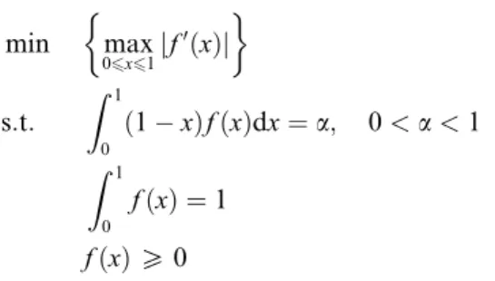
min VRIM¼ Z 1 0 FðfðxÞÞdx s:t: Z 1 0 ð1xÞfðxÞdx¼a; 0<a<1 Z 1 0 fðxÞdx¼1 fðxÞP0 ð42Þ
whereFis a strictly convex function in½0;þ1Þ,1and it is at least two order differentiable.
1
Similar to the OWA operator case, the feasible domain can beð0;þ1ÞifFis meaningless at 0 as in the case ofFðxÞ ¼xlnðxÞ. This means an implicit constraintfðxÞ>0 in the problem.
Asa¼0 ora¼1 correspond to the unique RIM quantifier generating function solution ofQðxÞandQðxÞ
respectively, we will not include these two special cases into the problem.
Theorem 8. IffðxÞis the optimal solution of(42)with given orness levela, thenfð1xÞis the optimal solution of
(42)with 1a.
Proof. With given orness levela, suppose the optimal solution of(42)isfðxÞ, then
R1
0ð1xÞfðxÞdx¼a
R1
0fðxÞdx¼1
(
We will show thathðxÞ ¼fð1xÞis the optimal solution of (42)with 1a. It can be verified that
R1 0ð1xÞhðxÞdx¼ R1 0ð1xÞfð1xÞdx¼ R1 0tfðtÞdt¼1a R1 0hðxÞdx¼ R1 0fð1xÞdx¼ R1 0fðtÞdt¼1 (
IfhðxÞ ¼fð1xÞis not the optimal solution of(42)with 1a, then there existsrðxÞ,rðxÞ 6¼hðxÞand
R1
0ð1xÞrðxÞdx¼1a
R1
0rðxÞdx¼1
(
which makes R01FðrðxÞÞdx<R01FðhðxÞÞdx¼R01Fðfð1xÞÞdx. It can verified thatrð1xÞsatisfies
R1 0ð1xÞrð1xÞdx¼a R1 0rð1xÞdx¼1 ( and Z 1 0 Fðrð1xÞÞdx¼ Z 1 0 FðrðtÞÞdt< Z 1 0 FðhðxÞÞdx¼ Z 1 0 Fðfð1xÞÞdx
This contradicts the assumption thatfðxÞis the optimal solution of(42)with orness levela. Sofð1xÞis
the optimal solution of (42)with 1a. h
Theorem 9. The optimal solution of(42)is unique, and it can be expressed as
fðxÞ ¼ gðk1xþk2Þ if x2E
0 otherwise
ð43Þ
where k1;k2is determined by the constraints of(45):
R Exgðk1xþk2Þdx¼1a R Egðk1xþk2Þdx¼1 ( ð44Þ and E¼ fxj06x61;gðk1xþk2ÞP0gwith gðxÞ ¼ ðF0Þ1ðxÞ.
Proof. An alternative form of Problem(42)is min Z 1 0 FðfðxÞÞdx s:t: Z 1 0 xfðxÞdx¼1a; 0<a<1 Z 1 0 fðxÞdx¼1 fðxÞP0 ð45Þ
min J¼ Z 1 0 FðfðxÞÞdx s:t: dw dx ¼ xfðxÞ fðxÞ x2 ½0;1 wð0Þ ¼ 0 0 ; wð1Þ ¼ 1a 1 ð46Þ
and the control constraintfðxÞP0.
AsFis strictly convex, with the optimal control theory[36], there exist an unique optimal solutionfðxÞfor
(46).
The Hamiltonian is
H¼FðfðxÞÞ þk1xfðxÞ þk2fðxÞ ð47Þ
SinceFis convex that F0is increasing,ðF0Þ1exists. The optimal solution has the following form:
fðxÞ ¼ ðF 0Þ1 ðk1xk2Þ if F01ðk1xk2ÞP0 0 otherwise ( ð48Þ
LetðF0Þ1ðxÞ ¼gðxÞ, and replacek1;k2 withk1;k2for simple expression,(48)becomes
fðxÞ ¼ gðk1xþk2Þ if x2E
0 otherwise
ð49Þ
wherek1;k2is determined by the constraints of (45):
R Exgðk1xþk2Þdx¼1a R Egðk1xþk2Þdx¼1 ( ð50Þ andE¼ fxj06x61;gðk1xþk2ÞP0g. h
AsR01Fðfð1xÞÞdx=R01FðfðxÞÞdx, fromTheorems 8 and 9, we can get that
Corollary 5. Let VRIMðaÞ ¼R01FðfðxÞÞdx be the objective function of orness level a for (42), then
VRIMðaÞ ¼VRIMð1aÞ, which meansVRIMðaÞis symmetrical for aat a¼12.
Theorem 10. k1;k2in(43) and (44)can be seen as the functions the orness levelawithk1ðaÞ;k2ðaÞ.k1ðaÞ
mono-tonically decreases with a and k2ðaÞ monotonically increases with a. The objective value of (42),
VRIMðaÞ ¼
R1
0Fðfðx;aÞÞdxis a convex function of orness levela.
Proof. WithTheorem 9, the parametersk1;k2in(43) and (44)can be uniquely determined by the orness level
a. Let us make a differential operation fora on the both sides of(44),
R Exg 0ðk 1xþk2Þðk01xþk 0 2Þdx¼ 1 R Eg 0ðk 1xþk2Þðk01xþk 0 2Þdx¼0 ( ð51Þ that is k01REx2g0ðk 1xþk2Þdxþk02 R Exg 0ðk 1xþk2Þdx¼ 1 k01RExg0ðk1xþk2Þxþk02 R Eg 0ðk 1xþk2Þdx¼0 ( ð52Þ
Solving these linear equations, k01¼ R Eg 0ðk 1xþk2Þdx R Ex 2g0ðk 1xþk2Þdx R Eg 0ðk 1xþk2Þdx R Exg 0ðk 1xþk2Þdx 2 k02¼ R Exg 0ðk 1xþk2Þdx R Ex 2g0ðk 1xþk2Þdx R Eg 0ðk 1xþk2Þdx R Exg 0ðk 1xþk2Þdx 2 8 > > > > > < > > > > > : ð53Þ Considering that Z E x2g0ðk1xþk2Þdx Z E g0ðk1xþk2Þdx Z E xg0ðk1xþk2Þdx 2 ¼1 2 Z E x2g0ðk 1xþk2Þdx Z E g0ðk1yþk2Þdyþ Z E y2g0ðk 1yþk2Þdx Z E g0ðk1xþk2Þdx 2 Z E xg0ðk1xþk2Þdx Z E yg0ðk1yþk2Þdy ¼1 2Eðx 22xyþy2Þg0ðk 1xþk2Þg0ðk1yþk2Þdxdy¼ 1 2EðxyÞ 2 g0ðk1xþk2Þg0ðk1yþk2Þdxdy
where E¼ fxj06x61;gðk1xþk2ÞP0g or E¼ fyj06y61;gðk1yþk2ÞP0g depends on the variable
name of the integrand function, and E¼ fðx;yÞj06x61;06y61;gðk1xþk2ÞP0;gðk1yþk2ÞP0g.
Then(53)becomes k01¼ 2 R Eg 0ðk 1xþk2Þdx EðxyÞ2g0ðk 1xþk2Þg0ðk1yþk2Þdxdy k02¼ 2R Exg 0ðk 1xþk2Þdx EðxyÞ2g0ðk1xþk2Þg0ðk1yþk2Þdxdy 8 > < > : ð54Þ
Sincegis an increasing function,g0P0 andEis not empty, it follows thatk0
1<0,k
0
2>0, sok1decreases with
a andk2 increases witha.
With(43)andg¼ ðF0Þ1, V0RIMðaÞ ¼ Z E F0ðfðx;aÞÞogðk1xþk2Þ oa dx¼ Z E F0ðgðk1xþk2ÞÞg0ðk1xþk2Þðk01xþk 0 2Þdx ¼ Z E ðk1xþk2Þg0ðk1xþk2Þðk01xþk 0 2Þdx ¼k1 Z E xg0ðk1xþk2Þðk01xþk 0 2Þdxþk2 Z E g0ðk1xþk2Þðk01xþk 0 2Þdx
Considering (51),V0RIMðaÞ ¼ k1, withk1 decreasing witha, soVRIMðaÞis a convex function fora. h
From Corollary 5andTheorem 10, it can be obtained that
Corollary 6. The objective function of orness levelafor(42),VRIMðaÞ ¼R01Fðfðx;aÞÞdxdecreases fora2 ð0;12,
and increases ina2 ½1
2;1Þ.VRIMðaÞÞreaches its minimum value ata¼12.
WithQðxÞ ¼R0xfðtÞdt, QðxÞ ¼
Z
D
gðk1tþk2Þdt; D¼ ftj06t6x;gðk1tþk2ÞP0g ð55Þ
It is obvious that the shape of fðxÞandQðxÞis determined by the orness levela. IfQðxÞis regarded as a
parameterized function family ofQðx;aÞ, it holds that
Theorem 11. For the RIM quantifier function Qðx;aÞ with orness level a, it holds that 8x2 ½0;1, Qðx;aÞ
monotonically increases with a, and furthermore, 8X ¼ ðx1;x2;. . .;xnÞ, the aggregation value FQðXÞ also
Proof. From(55), oQðx;aÞ oa ¼ Z D g0ðk1tþk2Þðk01tþk 0 2Þdt¼k 0 1 Z D tg0ðk1tþk2Þdtþk02 Z D g0ðk1tþk2Þdt
With(54), and replacing the integrand variablex;y ink01;k02 witht;s,E¼ fxj06x61;gðk1xþk2ÞP0g
be-comesE¼ ftj06t61;gðk1tþk2ÞP0g, then oQðx;aÞ oa ¼ 2RDtg0ðk1tþk2ÞdtREg0ðk1tþk2Þdt EðtsÞ 2 g0ðk 1sþk2Þg0ðk1tþk2Þdsdt þ 2 R Dg 0ðk 1tþk2ÞdtREtg0ðk1tþk2Þdt EðtsÞ 2 g0ðk 1sþk2Þg0ðk1tþk2Þdsdt AsD¼ ftj06t6x;gðk1tþk2ÞP0gis a subset of E,ED¼ ftjx6t61;gðk1tþk2ÞP0g, oQðx;aÞ oa ¼ 2RDtg0ðk1tþk2ÞdtREDg0ðk1tþk2Þdt EðtsÞ 2 g0ðk 1sþk2Þg0ðk1tþk2Þdsdt þ2 R Dg 0ðk 1tþk2ÞdtREDtg0ðk1tþk2Þdt EðtsÞ 2 g0ðk 1sþk2Þg0ðk1tþk2Þdsdt ¼2DðstÞg 0ðk 1sþk2Þg0ðk1tþk2Þdsdt EðstÞ 2 g0ðk 1sþk2Þg0ðk1tþk2Þdsdt where D¼ fðs;tÞjx6s61;06t6x;gðk1sþk2ÞP0;gðk1tþk2ÞP0g, E¼ fðs;tÞj06s61;06t61; gðk1sþk2ÞP0;gðk1tþk2ÞP0g.
Sinceg is an increasing function,g0P0, andsPton D,oQoaðx;aÞP0, andQðx;aÞincreases witha.
From (3), let us suppose that x1Px2P Pxn, then FQðXÞ ¼Pni¼1xi Q ni Q in1
¼xnQð1Þþ Pn1 i¼1ðxixiþ1ÞQ ni ¼xnþ Pn1 i¼1ðxixiþ1ÞQ ni . As 8i; i¼1;2;. . .;n1, xixiþ1P0 and 8x2 ½0;1,
Qðx;aÞincreases witha, soFQðXÞincreases with orness levela. h
Asg¼ ðF0Þ1
is an strictly increasing function, from(43),fðxÞis also is a monotonic function. Whether it is
increasing or decreasing depends on the sign ofk1. Furthermore, it can be obtained that
Corollary 7. For the RIM quantifierQðxÞand its generating functionfðxÞdetermined by the optimal solution(42)
with orness levela, ifa¼1
2, then k1¼0, fðxÞ ¼1, QðxÞ ¼x, and FQðXÞ ¼FQAðXÞ ¼ 1 n
Pn
i¼1xi. Ifa<12, then
k1>0,fðxÞis increasing, QðxÞ is convex and8X, FQðXÞ<FQAðXÞ ¼1nPni¼1xi. If a>12, then k1<0, fðxÞis
decreasing,QðxÞis concave and8X,FQðXÞ>FQAðXÞ ¼1nPni¼1xi.
Proof. Whenk1¼0, from(43),fðxÞbecomes a constant, withDefinition 2and(7),fðxÞ ¼1, anda¼12. From Theorem 10, k1 decreases with orness level a. So if a¼12, then k1¼0, fðxÞ ¼1, QðxÞ ¼x, and FQðXÞ ¼ FQAðXÞ ¼
1
n
Pn
i¼1xi.
Considering the decreasing property ofk1 with orness levela, whena>12,k1<0, thenfðxÞis decreasing,
QðxÞ is concave, from Theorem 11, 8X, FQðXÞ>FQAðXÞ ¼n1Pni¼1xi. When a<12, k1>0, then fðxÞ is
increasing,QðxÞis convex and8X,FQðXÞ<FQAðXÞ ¼1nPni¼1xi. h 4.2. The solution equivalence to the minimax problem
Corresponding to(42), consider the minimax problem for RIM quantifier:
min MRIM¼ max
06x61jF 00ðfðxÞÞf0ðxÞj s:t: Z 1 0 ð1xÞfðxÞdx¼a; 0<a<1 Z 1 0 fðxÞdx¼1 fðxÞP0 ð56Þ
Problem (42)minimizes the overall integral of FðfðxÞÞ, while (56)tries to minimize the absolute maximum
Theorem 12. IffðxÞis the optimal solution of(56)with given orness levela, thenfð1xÞis the optimal solution of (56)with1a.
Proof. Similar toTheorem 8, omitted. h
Theorem 13. There is an unique optimal solution for(56), and the optimal solutions of the two kinds problems(42) and (56)are the same. That is, they both have the form of(43)as
foptðxÞ ¼
gðk1xþk2Þ if gðk1xþk2ÞP0
0 otherwise
ð57Þ
where g¼ ðF0Þ1,k1;k2is determined by the constraints:
R1 0xfoptðxÞdx¼1a R1 0foptðxÞdx¼1 ( ð58Þ
Proof. We only need to prove thatfoptis the optimal solution of(56). Assume that there exists a functionfðxÞ
such that fðxÞ 6foptðxÞ; fðxÞP0; max 06x61jF 00ðfðxÞÞf0ðxÞj6max 06x61 F 00ðf optðxÞÞfopt0 ðxÞ ð59Þ
and the constraint R01fðxÞ ¼1. We will prove that fðxÞ does not satisfy the constraint R01ð1xÞfðxÞ ¼a.
From (57),
F00ðfoptðxÞÞfopt0 ðxÞ ¼ ðF0ðfoptðxÞÞ0¼
oF0ðgðk1xþk2ÞÞ ox x2E 0 otherwise ( ð60Þ whereE¼ fxj06x61;gðk1xþk2ÞP0g. Withg¼ ðF0Þ1,oF0ðgðk1xþk2ÞÞ ox ¼ oðk1xþk2Þ ox ¼k1, thus F00ðfoptðxÞÞfopt0 ðxÞ ¼ k1 x2E 0 otherwise ð61Þ
So max06x61jF00ðfoptðxÞÞfopt0 ðxÞj ¼ jk1j. As F00ðfðxÞÞf0ðxÞ ¼ ðF0ðfðxÞÞ0 and F00ðfoptðxÞÞfopt0 ðxÞ ¼ ðF0ðfoptðxÞÞ0, let
RðxÞ ¼F0ðfðxÞÞandRoptðxÞ ¼F0ðfoptðxÞÞ, from(59),
maxjR0ðxÞj6jR0optðxÞj ¼ jk1j x2E ð62Þ
WithTheorems 8 and 12, we will discuss in the following two cases. Case 1: If a¼1
2, from Corollary 7, k1¼0.foptðxÞ becomes a constant, E¼ ½0;1, fopt¼1. We also have
maxx2½0;1jR0ðxÞj ¼0, thenR0ðxÞ ¼ ðF0ðfðxÞÞÞ0¼0 forx2 ½0;1,F0ðfðxÞÞis a constant. AsFis convex, F0is increasing,fðxÞis also a constant. WithR01fðxÞdx¼1,fðxÞ ¼1, thusfðxÞ foptðxÞon [0, 1], this
is a contradiction. Case 2: Ifa6¼1
2. For simplification, we will only prove the case ofa<
1
2, the condition ofa> 1
2can be obtained
directly with the symmetrical property of Theorems 8 and 12.
From Corollary 7, if a<1
2, then k1>0. As g is a continuous and monotonic increasing function,
gðk1xþk2Þis also continuous and monotonic increasing,E¼ fxj06x61;gðk1xþk2ÞP0gis a continuous
and compact subset of [0, 1]. Let inffEg ¼a, and supfEg ¼b, then E¼ ½a;b and it has b¼1 and
fðaÞ ¼gðk1aþk2Þ ¼0 ifa6¼0. From(62),
We can claim thatRð1Þ<Roptð1Þ, otherwise,Rð1ÞPRoptð1Þ. As RðxÞ ¼Rð1Þ Z 1 x R0ðtÞdt RoptðxÞ ¼Roptð1Þ Z 1 x R0optðtÞdt ð64Þ
Combining (63) and (64), we will have RðxÞPRoptðxÞ on ½a;1, that is F0ðfðxÞÞPF0ðfoptðxÞÞ, so
fðxÞPfoptðxÞ, and
R1
a fðxÞdxP
R1
afoptðxÞdx. Considering that
R1
0foptðxÞdx¼
R1
afoptðxÞdx¼1, and
R1
0fðxÞ ¼1, fðxÞP0, we must have fðxÞ ¼foptðxÞ on ½a;1 and fðxÞ ¼0 on ½0;a, which imply that
fðxÞ foptðxÞon [0, 1]. This is a contradiction. So we must haveRð1Þ<Roptð1Þ.
Next, we will show that there existsx0 that makes
RðxÞPRoptðxÞ 8x2 ½0;x0
RðxÞ<RoptðxÞ 8x2 ðx0;1
ð65Þ
It will be proved with the two casesa>0 anda¼0 respectively.
Ifa>0, then foptðaÞ ¼0, withfðaÞP0, then fðaÞPfoptðaÞ ¼0, thusRðaÞPRoptðaÞ, considering(63),
(64)andRð1Þ<Roptð1Þ, there exists ax02 ½a;1Þ, that makes
RðxÞPRoptðxÞ 8x2 ½a;x0
RðxÞ<RoptðxÞ 8x2 ðx0;1
ð66Þ
Forx2 ½0;a, withfðxÞP0¼foptðxÞ, thenRðxÞPRoptðxÞ. Combining with(66),
RðxÞPRoptðxÞ 8x2 ½0;x0
RðxÞ<RoptðxÞ 8x2 ðx0;1
ð67Þ
Ifa¼0, we will show thatRð0ÞPRoptð0Þ, otherwiseRð0Þ<Roptð0Þ. Considering that
RðxÞ ¼Rð0Þ þ Z x 0 R0ðtÞdt RoptðxÞ ¼Roptð0Þ þ Z x 0 R0optðtÞdt ð68Þ
combining (63), we will have RðxÞ<RoptðxÞ on [0, 1], that is F0ðfðxÞÞ<F0ðfoptðxÞÞ, so fðxÞ<foptðxÞ, and
R1
0fðxÞdx<
R1
0foptðxÞdx. This contradicts with the condition that
R1
0fðxÞdx¼
R1
0foptðxÞdx¼1. With
Rð0ÞPRoptð0ÞandRð1Þ<Roptð1Þand(63), it can also be obtained that there exists ax02 ½0;1Þ, that makes
RðxÞPRoptðxÞ 8x2 ½0;x0
RðxÞ<RoptðxÞ 8x2 ðx0;1
ð69Þ
AsRðxÞ ¼F0ðfðxÞÞandRoptðxÞ ¼F0ðfoptðxÞÞ, andF0is strictly increasing, thus
fðxÞPfoptðxÞ 8x2 ½0;x0 fðxÞ<foptðxÞ 8x2 ðx0;1 ð70Þ WithR01foptðxÞdx¼ R1 0 fðxÞdx¼1, Z 1 0 ð1xÞfoptðxÞdx Z 1 0 ð1xÞfðxÞdx¼ Z x0 0 x½fðxÞ foptðxÞdxþ Z 1 x0 x½fðxÞ foptðxÞdx < Z x0 0 x0½fðxÞ foptðxÞdxþ Z 1 x0 x0½fðxÞ foptðxÞdx ¼x0 Z 1 0 ½fðxÞ foptðxÞdx¼0
That is R01ð1xÞfðxÞdx>R01ð1xÞfoptðxÞdx¼a, this contradicts the constraint R 1
0ð1xÞfðxÞdx¼a.
Therefore,foptðxÞis the optimal solution of (56), and the optimal solution is unique. h
From Theorems 12 and 13, we can get that
Corollary 8. Let MRIMðaÞ ¼max06x61jF00ðfðxÞÞf0ðxÞj is the objective function of orness level a for (56), then
MRIMðaÞ ¼MRIMð1aÞ, which meansVRIMðaÞis symmetrical foraat a¼1 2.
Theorem 14. The objective value of the minimax problem(56),MRIMðaÞ ¼max06x61jF00ðfðxÞÞf0ðxÞjdecreases for
a2 ð0;1
2, and decreases fora2 ½ 1
2;1Þ.MRIMðaÞreaches its possible minimum value 0 ata¼ 1 2.
Proof. From(61), with the unique optimal solution of(57) and (58), the objective function value of the
mini-max problem(56)is MRIMðaÞ ¼ max 06x61 F 00ðf optðxÞÞfopt0 ðxÞ ¼ jk1j ð71Þ
From Corollary 7, whena¼1
2,k1¼0,MRIMðaÞ ¼0. FromTheorem 10,k1decreases with orness levela, so
k1>0 for a2 0;12
, k1<0 for a2 12;1
, that MRIMðaÞ ¼ jk1j decreases for a2 0;12
, and it increases for
a2 1
2;1
,MRIMðaÞreaches its possible minimum value 0 ata¼12. h
5. The solutions of two special cases
Here we will discuss the solution expression of two special cases of (8) and (42)with FðxÞ ¼xlnðxÞ and
FðxÞ ¼x2, which correspond to the maximum entropy problem and the minimum variance problem
respec-tively. The solutions of these two problems in OWA operator case were discussed separately
[12,14,15,26,31,35]. The results of this paper can be seen as an extension of them and an effort of trying to
connect these two problems together [33]. Most properties of these two kinds problems for OWA operator
and RIM quantifier[24,26,27,31]can be deduced directly from the conclusions of this general model. Similar
to the conclusions in Sections3 and 4, the relationship between OWA operator and RIM quantifier can also
be observed and compared.
For the optimization problems(8), withPni¼1wi¼1,P
n
i¼1ðaFðwiÞ þbwiÞ ¼aP n
i¼1FðwiÞ þb, similarly, for
(42), with R01fðxÞdx¼1,R01ðaFðfðxÞÞ þbfðxÞÞdx¼aR01FðfðxÞÞdxþb, FðxÞ andaFðxÞ þbxða>0Þhave the
same optimal solutions for (8) and (42), so the parameters aða>0Þ;b in aFðxÞ þbx of (8) and (42)can be
neglected in some way. Please also note that the case ofFðxÞ ¼xlnðxÞis a maximum problem with an
addi-tional negative sign in the objective function. 5.1. Case 1:FðxÞ ¼xlnðxÞ
Problem (8)becomes the maximum entropy OWA (MEOWA) operator problem(72).
max X n i¼1 wilnwi s:t: X n i¼1 ni n1wi¼a; 0<a<1 Xn i¼1 wi¼1 ð72Þ
As F0ðxÞ ¼1þlnðxÞ,gðxÞ ¼ ðF0Þ1ðxÞ ¼ex1, from(10) and (11), the optimal solution is
Let wi
wiþ1¼e 1
n1k1¼1
q, the solution can be expressed in geometric form as[8,31]
wi¼ q i1 P n1 j¼0 qj ð73Þ
whereqis the unique positive real root of the following equation:
ðn1Þaqn1þX
n
i¼2
ððn1Þaiþ1Þqni¼0
With the relationship betweenk1andq, from the conclusions of Section3.1, we can also get the same
con-clusions about the MEOWA operator that were once obtained in[31].
Corresponding to(25), the solution equivalence minimax problem of(72)is
min max 16i6n1jlnðwiÞ lnðwiþ1Þj s:t: X n i¼1 ni n1wi¼a; 0<a<1 Xn i¼1 wi¼1: ð74Þ
Furthermore, the solution equivalence minimax problem(74)can be replaced with a more simple minimax
ratio problem(75)without the absolute value operator. Similar to the minimax disparity problem(24), we can
call(75)as minimax ratio problem, which minimizes the maximum of the ratios between two adjacent weight
elements.
Theorem 15. The solution of the maximum entropy problem (72) is also equivalent to the following minimax problem solution: min max 16i6n1 wi wiþ1 s:t: X n i¼1 ni n1wi¼a; 0<a<1 Xn i¼1 wi¼1 wiP0; i¼1;2;. . .;n ð75Þ
Proof. We will show that the optimal solution of maximum entropy OWA operator problem (72) with Wopt¼ ðwopt1 ;wopt2 ;. . .;wopt
n Þin (73)is also the unique optimal solution of(75).
LetW ¼ ðw1;w2;. . .;wnÞbe a OWA weight vector such thatW 6Wopt, and max 16i6n1 wi wiþ1 6 max 16i6n1 wopti woptiþ1¼ 1 q ð76Þ
and the constraintPni¼1wi¼1. We will prove thatwidoes not satisfy the constraintP
n
i¼1nni1wi¼a.
We claim thatwn>woptn , otherwise,wn6woptn . As
wi¼wn Yn1 k¼i wk wkþ1 ; wopti ¼w opt n qni fori¼1;2;. . .;n ð77Þ
considering(76), we haveQnk¼i1 wk
wkþ1 6 1 qni, so wi6w opt i ;i¼1;2;. . .;n. Since Pn i¼1wi¼P n i¼1w opt i ¼1, we must
Similarly, with wi¼w1 Yi1 k¼1 wk wkþ1 , ; wopti ¼wopt1 qi1; i¼1;2;. . .;n ð78Þ
we can also prove thatw1<wopt1 . Combining these with(77) and (76), we can find k, 1<k6n, such that
wi6w opt i i¼1;2;. . .;k1 wi>w opt i i¼k;kþ1;. . .;n (
With the same proof method as Theorem 6 after (40), we can obtain that Pni¼1nni1wi<
Pn i¼1 ni n1w opt i ¼a. Therefore,Wopt¼ ðwopt1 ;wopt
w ;. . .;w
opt
n Þis the unique optimal solution of(75). h
Remark 2. Similarly, the objective function in(75)can also be replaced with min max16i6n1wwiþi1
n o
.
For Problem(42), whenFðxÞ ¼xlnðxÞ, it becomes the maximum entropy RIM quantifier problem (79).
max Z 1 0 fðxÞlnfðxÞdx s:t: Z 1 0 ð1xÞfðxÞdx¼a; 0<a<1 Z 1 0 fðxÞdx¼1: ð79Þ
The solution and its properties were discussed in[27].
WithF0ðxÞ ¼1þlnðxÞ,ðF0Þ1ðxÞ ¼ex1, as ex1>0, from(43) and (44), the optimal solution is:
fðxÞ ¼ek1xþk21
With the constraints of(79), the optimal solution can be expressed as
fðxÞ ¼ k1e k1x
ek11
wherek1is the root of the equatione
k1k
11
k1ðek11Þ¼a.
Remark 3. In[27], the solution of the maximum entropy RIM quantifier is expressed asfðxÞ ¼kekð1xÞ
ek1, wherek
is the root of the equationkekekþ1
kðek1Þ ¼a. It can be easily verified that these two solution forms are equivalent
withk¼ k1.
AsF00ðxÞ ¼1
x, corresponding to(56), the solution equivalence minimax problem of(79)is:
min max 06x61j f0ðxÞ fðxÞj s:t: Z 1 0 ð1xÞfðxÞdx¼a; 0<a<1 Z 1 0 fðxÞdx¼1 fðtÞ>0 ð80Þ
Furthermore, as in the discrete case of OWA operator,(80)can be replaced with a problem without
abso-lute value operator.
Theorem 16. The solution of the maximum entropy problem (79) is also equivalent to the following minimax problem solution without the absolute value operator.
min max 06x61 f0ðxÞ fðxÞ s:t: Z 1 0 ð1xÞfðxÞdx¼a; 0<a<1 Z 1 0 fðxÞdx¼1 fðtÞ>0 ð81Þ
Proof. We will show that the optimal solution of maximum entropy OWA operator problem(79),foptðxÞis
also the unique optimal solution of(81).
LetfðxÞbe a RIM quantifier such thatfðxÞ 6fopt, and
max 06x61 f0ðxÞ fðxÞ60max6x61 fopt0 ðxÞ foptðxÞ ¼k1 ð82Þ
and the constraintR01fðxÞ ¼1. We will prove thatfðxÞdoes not satisfy the constraintR01ð1xÞfðxÞdx¼a.
We claim thatfð0Þ>foptð0Þ, otherwise,fð0Þ6foptð0Þ.
LetRðxÞ ¼lnðfðxÞÞ,RoptðxÞ ¼lnðfoptðxÞÞ, thenRð0Þ6Roptð0Þ, andR0ðxÞ ¼ f0ðxÞ fðxÞ, furthermore, forx2 ½0;1, R0optðxÞ ¼f 0 optðxÞ foptðxÞ¼k1. Considering (82), R0ðxÞ6R0optðxÞ ¼k1 8x2 ½0;1 ð83Þ
As in Case 2 of theTheorem 13proof, it can be proved that there existsx0, which makes
RðxÞ6RoptðxÞ 8t2 ½0;x0 RðxÞ>RoptðxÞ 8t2 ðx0;1 ð84Þ thus fðxÞ6foptðxÞ 8t2 ½0;x0 fðxÞ>foptðxÞ 8t2 ðx0;1 ð85Þ
and R01ð1xÞfðxÞdx<R01ð1xÞfoptðxÞdx¼a at last, which contradicts the constraint
R1
0ð1xÞfðxÞdx¼a.
Therefore,foptðxÞis the unique optimal solution of(81). h
5.2. Case 2:FðxÞ ¼x2
Problem(8)becomes the alternative form of the minimum variance problems for OWA operator[15]:
min D2ðWÞ ¼1 n Xn i¼1 w2i 1 n2 s:t: X n i¼1 ni n1wi¼a; 0<a<1 Xn i¼1 wi¼1; wiP0; i¼1;2;. . .;n: ð86Þ AsF0ðxÞ ¼2x,ðF0Þ1ðxÞ ¼x
2, the optimal solution is:
wi¼ ni n1k1þk2 2 if ni n1k1þk2 2 >0 0 otherwise ( ð87Þ
with Pn i¼1 ni n1wia¼0 Pn i¼1 wi1¼0 8 > > < > > : ð88Þ
We will discuss the determination ofW ¼ ðw1;w2;. . .;wnÞin different cases.
Case 1: IfaP1
2. The OWA operator weight vector has the formW ¼ ðw1;w2;. . .;wm;0;0;. . .;0Þ, wheremis
the nonzero elements ofW. Observing thatm¼1 corresponds to the unique caseW¼ ð1;0;. . .;0Þof
a¼1, we will assumemP2 in the following. From(88), it can be obtained that
k1¼ 12ðn1Þð2nþ2anþ12aþmÞ mðm1Þðmþ1Þ k2¼4ð6n 2þ6an29anþ6nþ6mn3man1þ3maþ3a2m23mÞ mðm1Þðmþ1Þ 8 < : ð89Þ Withwm¼nm n1k1þk2>0 and nðmþ1Þ
n1 k1þk260 ðmP2Þ, we can get that
3nm1
3ðn1Þ >aP
3nm2
3ðn1Þ ð90Þ
This is the orness interval alies in when Whasmnonzero elements for aP1
2. Observing that when
m¼2;3;. . .;n,aonly changes in½2
3;1Þ, we can get a division of½
2
3;1Þform¼1;2;. . .;n.. It is obvious
that when all thewis are nonzero, we havem¼n. From(90), fora2 1
2; 2 3
, it certainly hasm¼n. Thus,
with given orness levela2 ½1
2;1Þ,mcan be determined as m¼ ½3n3ðn1Þa1 a2 2 3;1 n a2 1 2; 2 3 ( ð91Þ Case 2: Ifa<1
2. The OWA operator weight vector has the formW ¼ ð0;0;. . .;0;wnmþ1;wnmþ2;. . .;wnÞ.m
can be determined in a similar way
m¼ ½3ðn1Þaþ2 a2 0; 1 3 n a2 ½1 3; 1 2Þ ( ð92Þ
Combining(87), (91) and (92), the solution is the maximum spread equidifferent OWA operator exactly
[26]: Algorithm 1
Step1: Determine mwith(93).
m¼ ½3aðn1Þ þ2 if 0<a<1 3 n if 1 36a6 2 3 ½3n3aðn1Þ 1 if 2 3<a<1: 8 > < > : ð93Þ
Step2: Determine dwith(94).
d¼ 6ð2a2naþm1Þ mðm21Þ if 0<a<13 6ð12aÞ nðnþ1Þ if 1 36a6 2 3 6ð2a2naþ2nm1Þ mðm21Þ if 23<a<1 8 > > > < > > > : ð94Þ
Step3: DetermineW ¼ ðw1;w2;. . .;wnÞwith(95). Case 1: 0<a<1 3; wi¼ 0 if 16i6nm dm2þdmþ2 2m þ ðinþm1Þd if nmþ16i6n ( Case 2: 1 36a6 2 3; wi¼ dn2þdnþ2 2n þ ði1Þd; i¼1;2;. . .;n Case 3: 2 3<a<1; wi¼ dm2þdmþ2 2m þ ði1Þd if 16i6m 0 if nmþ16i6n ( ð95Þ
Similar to the maximum entropy problem, the properties of minimum variance problem that was proposed
in[26]can also be obtained from the discussion of Section3.1. The similarities between the maximum entropy
and the minimum variance problems can be understood naturally as they are just two special cases of the
gen-eral problem(8).
WithTheorem 6andFðxÞ ¼x2, the solution equivalence minimax problem of(86)and the minimax
dispar-ity problem(24)can be verified with an additional constant 2 in(24)’s objective function, which improves the
complicated process of the dual linear programming method[30].
For the RIM quantifier case, whenFðxÞ ¼x2, problem(42)becomes the minimum variance RIM operator
problem[24]: min D2ðfðxÞÞ ¼ Z 1 0 f2ðxÞdx Z 1 0 fðxÞdx 2 s:t: Z 1 0 ð1xÞfðxÞdx¼a 0<a<1 Z 1 0 fðxÞ ¼1 fðxÞP0 ð96Þ
Problem(96)can be solved with the optimal control technique. The solution is expressed as an equidifferent
RIM quantifier. Some properties of it were discussed[24].
AsF0ðxÞ ¼2x,ðF0Þ1ðxÞ ¼x
2, the optimal solution is:
fðxÞ ¼ k1xþk2 2 if k1xþk2 2 P0 0 otherwise ( with R1 0xfðxÞdx¼1a R1 0fðxÞdx¼1 (
This is just the equidifferent RIM quantifier[24]. The optimal solution is
Case 1: If 0<a61 3;fðxÞ ¼ 0 06x613a 2ðx1þ3aÞ 9a2 13a<x61 ( Case 2: If 1 3<a6 2 3;fðxÞ ¼ ð612aÞxþ ð6a2Þ; 06x61 Case 3: If 2 3<a<1fðxÞ ¼ 2ð33axÞ 9ð1aÞ2 06x633a 0 33a<x61 ( ð97Þ
AsF00ðxÞ ¼2, corresponding to(56), the solution equivalence minimax problem of(96)is formulated with