http://www.ams-mss.org
MODELLING AND SIMULATION
eISSN 2600-8084 VOL 1, NO. 1, 2017, 29-35Modelling and Control of DWR 1.0 – A Two
Wheeled Mobile Robot
Nurhayati Baharudin, Mohamad Shukri Zainal Abidin
*, Muhd Saiful Azimi Mahmud and Muhammad Khairie
Idham Abd Rahman
1Department of Control and Mechatronics Engineering, Faculty of Electrical Engineering, Universiti Teknologi Malaysia,
81310 UTM Johor Bahru, Johor, Malaysia.
*Corresponding author: [email protected]
Abstract: This paper presents modelling and control of DWR 1.0, a two wheeled mobile robot. This balancing robot is one of the applications of an inverted pendulum on a two wheel. A relatively recent offshoot of the classical inverted pendulum is the wheel inverted pendulum, popularized in contemporary culture by the Segway Personal Transporter. However, the mathematical model for a wheel inverted pendulum do not account for the full complexity of the construction of the platform. The mathematical model obtained in this work with the measured parameters is simulated using Matlab and PID control parameters are determined. Finally, PID control algorithm is implemented on the two-wheeled mobile robot to test the accuracy of the model.
Keywords: Inverted pendulum; modelling; PID control; simulation; two wheeled mobile robot.
1. INTRODUCTION
A two-wheel mobile robot is one of the applications for the inverted pendulum system. Inverted pendulum is a classical model of under-actuated, non-linear and unstable system. Hence, control of a two-wheel mobile robot is very challenging as it is non-linear, unstable and uncontrollable system. Research and study on the controlling self-balancing two-wheel robot has contributed to the practical interest which is the applications on the vehicle field and autonomous robotics. Many practical systems have been implemented based on the two-wheel self-balancing robot models [1]. Among these applications, Segway PT has been a popular personal transporter since invented in 2001[2].
The two-wheel mobile robots can be divided into two parts. The first is the lower parts which consist of two wheels connected to the axis and driven independently. The second part is the body of the robot which is placed at the centre of mass above the axis. The controller drives the wheel to maintain the body on the up-right position. Two wheeled mobile robots are well suited for traversing narrow spaces and slopes. Its characteristic includes compact size, light weight and lower energy consumption [3].
In this work, a two-wheeled mobile robot has been successfully developed, and this paper present development of the mathematical model. The mathematical model for the robot has to be developed based on the available system and hardware. By using the system identification approach, analysis of the physical platform, and the fundamental laws of mechanics, a non-linear model of the system can be developed. This is useful as various control techniques can be tested and simulated by using the developed model.
2. MATHEMATICAL MODEL
In this work, a non-linear model of DWR 1.0, a two wheeled mobile robot shown in Figure 1 is developed. The motion of these two wheels mobile robot system involve of translational and rotational movements. The mathematical model is then linearized and converted into a state space form.
2.1 DC Motor Modelling
The two-wheel mobile robot is powered by two DC motors. Figure 2 shows the diagram of a DC motor, and the mathematical model for the DC motor is derived [3].
Figure 1. The DWR 1.0 two wheeled mobile robot.
Figure 2. DC motor
The motor produces a torque which proportional to the current,
m k im
(1)
The voltage is proportional to the motor speed,
e e
V k (2)
According to Kirchhoff’s Voltage Law, sum of all voltages in the circuit must be equal to zero. 0 a di V Ri L dt (3)
By rearranging Equations (1), (2) and (3), the DC motor equation can be obtained as 1 m e a a R R R k k d V dt I R I R I (4) 2.2 Wheel Modelling
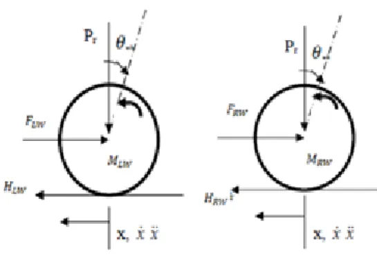
Figure 3 shows the free body diagram for left and right wheels. The free body diagram is useful to obtain the mathematical model based on Newton’s Law. Every wheel has its own DC motor, which will provide free movement.
Both of the wheels are assumed as identical and no slip occurs between wheels and ground. The mathematical modeling of wheel is described by the two motions which involve linear and angular motions.
Linear Motion .. LW LW LW LW x M H F (5) Angular Motion .. LW JLW TLW HLWR
(6) Left Wheel .. .. LW LW LW LW LW LW T J F x M R R
(7) Right Wheel .. .. RW RW RW RW RW RW T J F x M R R (8)By combining Equations (7) and (8), and rearranging the equations and substituting the parameters from the DC motor derivation section, The final equation for wheel modelling is obtained as
.. . : 2 2 2 2 WH WH m e m LW m RW ( LW RW) J k k k k M x x Va Va F F rR rR R rR (9) 2.3 Chassis Modelling
The body of the robot can be modelled as an inverted pendulum on the two wheels. The physical representation of the system is illustrated by a two wheel inverted pendulum. The model adopted here is based on [4], where the behavior can be influenced by the motor’s torque and disturbance forces from the centre of gravity. Figure 4 illustrates the free body diagram used to derive the mathematical model. Table 1 describes the symbols used in this paper.
The force balance equation can be written as
.. ..
cos ( 2 )
LW RW p p RC p WH
F F f M l M M M x (10)
From wheel modelling equation,
.. .. 2 2 cos 4 RW LW WH p p RC p WH T T J f M l M M M x R R R (11)
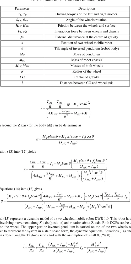
Table 1. Parameter of the two-wheeled mobile robot
Parameter Description
TL, TR Driving torques of the left and right motors.
θLW, θRW Angle of the wheels rotation.
HLW, HRW Friction between the wheels and surface
FL, FR Interaction force between wheels and chassis
fp External disturbance at the centre of gravity x Position of two-wheel mobile robot θ Tilt angle of inverted pendulum (robot body)
Mp Mass of pendulum
MRC Mass of robot chassis
MLW, MRW Masses of both wheels
R Radius of the wheel
CG Centre of gravity
l Distance between CG and wheel axis
Collecting, .. .. 2 cos 2 4 RW LW p WH WH RC T T fp M l R R x J M M M R (12)
Then, the rotation around the Z axis (for the body tilt) can be determine as ..
.. sin cos cos
( ) p p p MC MP M gl M x l f l J J
(13)Substituting Equation (13) into (12) yields
.. 2 2 2 2 sin cos cos ( ) cos 2 4 ( ) p p RW LW p p MC MP p WH WH RC Mp MC JMP M gl f l T T f M l R R J J x M l J M M M J J R (14)
and substituting Equations (14) into (12) gives
2 .. 2 2 2 2sin cos 4 cos
4 cos WH RW LW p p WH RC p p p WH MC MP WH RC p p J T T M gl f l M M M M l f R R R J J J M M M M l R (15)
Equations (14) and (15) represent a dynamic model of a two wheeled mobile robot DWR 1.0. This robot have two degrees of freedom (DOFs) involving movement along X-axis (position) and rotation about Z-axis. Both DOFs can be controlled via the DC motor setup on the wheel. The upper part or inverted pendulum is carried on top of the two wheels with length, l and weight, m. In order to represent the system in a state space form, the dynamic equations, Equations (14) and (15) need to be linearized. This was done using the Taylor’s series and with the assumption of small θ, (θ ≈ 0),
2 2 2 2 .. MC MP p p RW LW p MC MP MC MP J J M l M gl T T x f R
R
J J J J
(16)
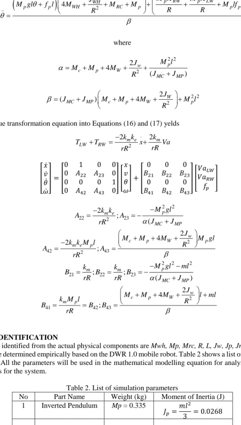
2 .. 4 p RW p LW WH p p WH RC p p p M lT M lT J M gl f l M M M M lf R R R (17) where 2 2 2 2 4 ( ) p w c p W MC MP M l J M M M J J R
2 2 2 2 ( MC MP) c p 4 W W p J J J M M M M l R Substituting the torque transformation equation into Equations (16) and (17) yelds . 2 2 m e 2 m LW RW k k k T T x Va rR rR (18) [ 𝑥̇ 𝑣̇ 𝜃̇ 𝜔̇ ] = [ 0 1 0 0 0 𝐴22 𝐴23 0 0 0 0 1 0 𝐴42 𝐴43 0 ] [ 𝑥 𝑣 𝜃 𝜔 ] + [ 0 0 0 𝐵21 𝐵22 𝐵23 0 0 0 𝐵41 𝐵42 𝐵43 ] [ 𝑉𝑎𝐿𝑊 𝑉𝑎𝑅𝑊 𝑓𝑝 ] 2 2 22 2 23 2 ; ( p m e MC MP M gl k k A A J J rR
2 42 2 43 2 4 2 ; w c p W p m e p J M M M M gl k k M l R A A rR 2 2 2 21 ; 22 ; 23 ( ) p m m MC MP M gl ml k k B B B rR rR
J J 2 41 42 43 2 4 ; w c p W m p J M M M l ml k M l R B B B rR 3. PARAMATER IDENTIFICATIONThe parameters to be identified from the actual physical components are Mwh, Mp, Mrc, R, L, Jw, Jp, Jm, km, ke, and r. These parameters need to be determined empirically based on the DWR 1.0 mobile robot. Table 2 shows a list of parameters identified from the DWR 1.0. All the parameters will be used in the mathematical modelling equation for analysis of the stability and design the controllers for the system.
Table 2. List of simulation parameters
No Part Name Weight (kg) Moment of Inertia (J) 1 Inverted Pendulum Mp = 0.335 𝐽𝑝= 𝑚𝑙2 3 = 0.0268 2 Chassis Mrc =0.65 𝐽𝑚= 1 12𝑚(𝑤2+ ℎ2) 3 Wheel Mwh = 0.245 𝐽𝑤= 1 12(𝑚𝑅2)
The DWR 1.0 robot is equipped with Pittman GM 8712-31 DC motor as the actuator. This motor is used to balance the robot with 24 V voltage supply. Table 4 shows the DC motor parameters identified using experiments.
Table 3. DC motor parameters
Battery Voltage (V) Current (A) RPM shaft (rad/sec) Voltage drop (V) Ke (V/rad/sec)
10 0.10 63 (6.597) 1.49 0.0213
15 0.12 100 (10.47) 1.788 0.0209
20 0.13 136 (14.24) 1.937 0.0210
24 0.15 167 (17.49) 2.235 0.0210
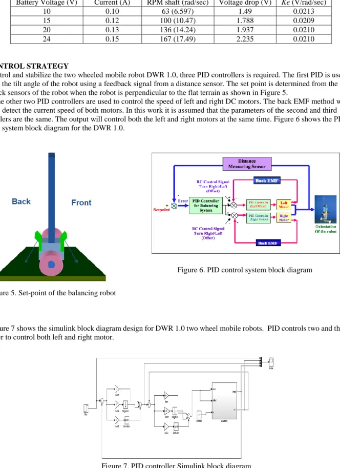
4. CONTROL STRATEGY
To control and stabilize the two wheeled mobile robot DWR 1.0, three PID controllers is required. The first PID is used to control the tilt angle of the robot using a feedback signal from a distance sensor. The set point is determined from the front and back sensors of the robot when the robot is perpendicular to the flat terrain as shown in Figure 5.
The other two PID controllers are used to control the speed of left and right DC motors. The back EMF method was used to detect the current speed of both motors. In this work it is assumed that the parameters of the second and third controllers are the same. The output will control both the left and right motors at the same time. Figure 6 shows the PID control system block diagram for the DWR 1.0.
Figure 5. Set-point of the balancing robot
Figure 6. PID control system block diagram
Figure 7 shows the simulink block diagram design for DWR 1.0 two wheel mobile robots. PID controls two and three join together to control both left and right motor.
Figure 7. PID controller Simulink block diagram 5. RESULT
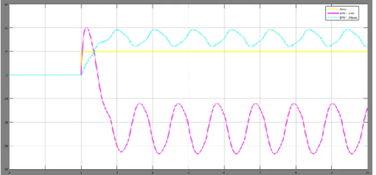
This PID controller was designed in a cascade, where each PID controller has their own input and position in series forming a single regulating device. In a cascade control loop, it has two types of controller, namely the master or primary and the secondary or the slave. The master PID controller generated a control signal that served as the set point to the slave PID. The slave PID in turn used the actuator to apply its control signal directly to the system. Table 4 shows the parameter values of Kp,
Ki and Kd for both the master and slave PID controllers. Figure 8 shows the response of the two wheeled mobile robot using
the proposed PID cascade control.
Figure 8. Simulation result using PID controller.
Table 4. PID controller parameters
Controller PID parameter values
Kp Ki Kd
PID 1 (tilt angle control) 4 0 0 PID 2 (left wheel speed control) 300 0.25 1 PID 3 (right wheel speed control) 300 0.25 1
The result showed that the system was oscillatory and unstable. A properly PID tuning with correct parameters are required. In addition, in the cascade control the secondary loop must be three or four times faster than the primary loop.
6. CONCLUSION
A mathematical model of a two wheeled mobile robot has been developed based on DWR 1.0. The actual parameters were determined experimentally and model was developed using the Newton Euler’s Method. For control of DWR 1.0, a cascade PID control technique was designed and simulation was performed within the MATLAB/Simulink environment. Simulation results have shown that a properly tuned PID controller is crucial. In addition, some efforts are needed to ensure that the system parameters obtained through experiments are correct.
REFERENCES
[1] C. T. Ching, Y. J. Shang and M. H. Shih, Trajectory tracking of self-balancing two-wheeled robot using back stepping sliding mode control and fuzzy basis function networks, Proceeding of the 2010 IEEE/RSJ International Conference on Intelligent Robots and system, Taipei, Taiwan, 2010, pp. 3943-3948.
[2] C. L. Shui, C. T. Ching and C. H. Hsu, Nonlinear adaptive sliding mode control design for two wheeled human transportation vehicle, Proceeding of the 2009 IEEE International Conference on Systems, Man and Cybernetics, San Antonio, USA, 2009, pp. 1965-1970.
[3] C. O. Rich, Balancing a two wheeled autonomous robot, Thesis, University of Western Australia, 2003
[4] A. O. Abd-Al-Azeem, M. K. Mohammed, R. A. Moukarrab and M. S. Ibraheem, TWIP robot balancing a two wheeled robot, Master of Science Thesis, University of Minia, 2009.