Risk-Based Comparison of Classification Systems

(1)

Air Force Institute of Technology Air Force Institute of Technology

AFIT Scholar

Theses and Dissertations Student Graduate Works

3-2008

Risk-Based Comparison of Classification Systems

Seth B. Wagenman

Follow this and additional works at: https://scholar.afit.edu/etd

Part of the Applied Mathematics Commons, and the Risk Analysis Commons

Recommended Citation Recommended Citation

Wagenman, Seth B., "Risk-Based Comparison of Classification Systems" (2008). Theses and Dissertations. 2659.

https://scholar.afit.edu/etd/2659

(2)

AFIT/GAM/ENC/08-01

RISK-BASED COMPARISON OF CLASSIFICATION SYSTEMS

THESIS

Seth B. Wagenman, Second Lieutenant, USAF AFIT/GAM/ENC/08-01

DEPARTMENT OF THE AIR FORCE AIR UNIVERSITY

AIR FORCE INSTITUTE OF TECHNOLOGY

Wright-Patterson Air Force Base, Ohio

(3)

The views expressed in this thesis are those of the author and do not reflect the official policy or position of the United States Air Force, Department of Defense, or the United States Government.

(4)

AFIT/GAM/ENC/08-01

RISK-BASED COMPARISON OF CLASSIFICATION SYSTEMS

THESIS

Presented to the Faculty

Department of Mathematics and Statistics Graduate School of Engineering and Management

Air Force Institute of Technology Air University

Air Education and Training Command In Partial Fulfillment of the Requirements for the

Degree of Master of Science

Seth B. Wagenman, B.S. Second Lieutenant, USAF

March 2008

(5)

AFIT/GAM/ENC/08-01

RISK-BASED COMPARISON OF CLASSIFICATION SYSTEMS

Seth B. Wagenman, B.S. Second Lieutenant, USAF

Approved:

Steven N. Thorsen (Chair) Date

Mark E. Oxley (Member) Date

(6)

AFIT/GAM/ENC/08-01

Abstract

Performance measures for families of classification system families that rely upon the analysis of receiver operating characteristics (ROCs), such as area under the ROC curve (AUC), often fail to fully address the issue of risk, especially for classification systems involving more than two classes. For the general case, we denote matrices of class prevalences, costs, and class-conditional probabilities, and assume costs are subjectively fixed, acceptable estimates for expected values of class-conditional probabilities exist, and mutual independence between a variable in one such matrix and those of any other matrix. The ROC Risk Functional (RRF), valid for any finite number of classes, has an associated parameter argument, that which specifies a member of a family of classification systems, and which system minimizes Bayes risk over the family. We typify joint distributions for class prevalences over standard simplices by means of uniform and beta distributions, and create a family of classification systems using actual data, testing independence

assumptions under two such class prevalence distributions. We minimize risk under two different sets of costs.

(7)

Acknowledgments

I would like to sincerely thank Maj Steve Thorsen for his patience while guiding this research, as well as Dr. Mark Oxley and Maj Dave Kaziska for their help in presenting it. I would also like to thank Dr. Ken Bauer and Maj Sam Wright for always being there to aid in reality-checking my implementation of these concepts, and Dr. Aihua Wood and Dr. Matt Fickus for helping me to know that the Theorems in the Appendix can be proved for all positive integers, for providing me with the confidence and ability to prove one of them fully, and for comforting me with the thought that someone else has probably already proved the other one for integers greater than 47.

Most importantly, I thank God for helping me to see things I never could have without His help, and for giving me my dear wife, who listened to my incessant babbling about this thesis and endured many a lonely evening whilst I fought with my computer, and who generally motivated, inspired, encouraged, and enabled me to seek education at the graduate level.

A note of thanks is also in order to the Air Force Office of Scientific Research for supporting our research efforts.

(8)

List of Figures

Figure Page

1. Standard 2-Simplex . . . 19

2. Standard 3-Simplex . . . 19

3. ROC Curve for One ROC Point Estimate . . . 24

4. Two ROC Curves with Equal AUC . . . 27

5. Bivariate General Beta Approximation to Normal over Standard 2-Simplex . . . 38

6. Standard Symmetric Beta Distribution as Normal(1₂,1₆) Approximation 38 7. General Symmetric Beta Distribution as Normal(1₄,₄₈1) Approximation 39 8. First Two Principal Component Scores, Fisher Iris Data . . . 40

9. Bayes Risks for Cost Regime 1 , Uniform Application . . . 44

10. Bayes Risks for Cost Regime 1 , Uniform Application . . . 44

11. Actual Error Rates, Uniform Application . . . 45

12. Bayes Risks for Cost Regime 1 , Beta Application . . . 46

13. Bayes Risks for Cost Regime 1 , Beta Application . . . 47

(10)

List of Tables

Table Page

1. Two-Class Contingency Matrix . . . 13

2. Two-Class Confusion Matrix . . . 14

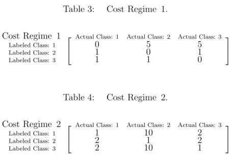
3. Cost Regime 1 . . . 43

4. Cost Regime 2 . . . 43

5. Mean Absolute Correlations and p-values, Uniform Application . . . . 46

(11)

List of Notations or Symbols

Notation or Symbol Meaning

1. AER Actual Error Rate

2. AUC Area Under the ROC Curve

3. FN False Negative Count

4. fnr False Negative Rate

5. FP False Positive Count

6. fpr False Positive Rate

7. h, iF Frobenius Dot Product

8. ⊙ Hadamard Matrix Product

9. PCA Principal Components Analysis

10. PNN Probabilistic Neural Net

11. ROC Receiver Operating Characteristic

12. ROCCH ROC Convex Hull

13. RRF ROC Risk Functional

14. ∆m Standard m-Simplex

15. TN True Negative Count

16. tnr True Negative Rate

17. TP True Positive Count

18. tpr True Positive Rate

(12)

RISK-BASED COMPARISON OF CLASSIFICATION SYSTEMS

I. Introduction and Mathematical Foundations

The concept of risk is a major feature of Bayesian decision theory [5, pp. 24-28], [18, p. 437]. Its power is evident in that it takes into account not only the relative severity of expected conditional losses for each possible decision, but also the likelihood of events upon which the occurrence of each loss is conditioned. It allows definition of these quantities through the use of either discrete or continuous random variables, or a combination of both. In this way, it accounts for many characteristics of the operating environment.

The term Receiver Operating Characteristic (ROC) seems to refer directly to this type of decision-theoretical framework, yet practical applications of decision theory in which this term appears often ignore critical aspects of Bayesian theory. To show this, a brief introduction to ROC analysis is necessary, as is a precise set of mathematical definitions, to establish a framework for possible correction of these oversights.

1.1 Introduction

The field of Receiver Operating Characteristic analysis emerged in the 1940s, during early attempts to discern between the presence or absence of signals amidst noise [6, pp. 1-2]. Since there are only two possible outcomes, such a signal detection process is an example of two-class or binary classification.

In signal detection, there are two possible classification errors—falsely perceiving the presence of signals amidst noise when there is only noise, and failing to detect a signal in

(13)

the midst of noise. One representation of the ROC for a binary classification system is simply a vector of the likelihoods of these errors. If the method of classification changes, so may these likelihoods, thereby generating a different ROC vector. A collection of estimates for such ROC vectors plotted on a unit square may offer limited visual insight into

comparison of the classification methods whose characteristic behavior they represent, and even more when other factors of interest are plotted on a third axis [10]. Many authors have developed advanced geometrical frameworks relating to the points so plotted, due to the common practice of calculating areas under a curve constructed of these plotted points [8], [10], [12], [13], [14], [21], [22], [26], [34], [36]. The use of ROCs in such comparative decision-making is referred to as ROC analysis.

Even though ROC analysis is used in many fields to compete binary classification techniques, it appears that very few of its proponents have fully realized the importance and potential of risk-based comparison as a tool for comparing classification techniques, especially those in which there are more than two distinct classes [30, pp. 57-64], [31, p. 352], [32, p. 4]. Although practical risk-based comparison of classification systems requires what could be considered unrealistic independence assumptions to enable the risk

calculations, the possible insights gained when these assumptions are met may at least justify the expense of testing them, and when viewed in light of the implicit assumptions connected with a failure to fully consider all elements of the risk calculation, these

assumptions may not be harsh at all. Since the failure to meet these assumptions is rarely mentioned in modern ROC analysis literature, the reason for not calculating risk may simply be the lack a practical and rigorous mathematical framework for its analysis. There is recent work, however, which constitutes a foundation on which to build a framework for

(14)

measuring the performance of classification systems, with Bayes risk as the measure of optimality, and incorporating some of the independence assumptions mentioned above [32]. The intent of this thesis is neither to show how these assumptions may be met, nor to stipulate as to the relative importance of actually meeting them, but instead to show how they may be tested, and then to assume that even if they are not met, the disadvantage of such failure is mitigated by the ability to easily calculate risk. The major point of interest is that geometric analyses are replaced by risk-based comparisons, thereby possibly

lessening the need to construct curves or surfaces, or to calculate geometric quantities.

1.2 Definitions and Assumptions

Before proceeding, it is necessary to define notation and terms relating to general classification theory and ROC analysis. Examples from the field of signal detection will illustrate selected concepts.

Definition 1 (Experiment). An experiment is a complex of reproducible conditions

resulting in a set of well-defined outcomes [16, pp. 3-5], [29, p. 32].

For example, the presence of electromagnetic radiation constitutes a possible signal detection experiment.

Definition 2 (Elementary Event). An elementary event is an experimental outcome which

cannot be further decomposed into other, more basic experimental outcomes [33, p. 26]. An elementary event in signal detection could be e = a detectable instance of electromagnetic radiation exists.

Definition 3 (Event Set). An event set is the set E =©eλ

ª

(15)

events resulting from a given experiment, where the index set Λ may be uncountable [16, pp. 3-5], [29, p. 33], [33, p. 27].

Definition 4 (Sensor, Data Set). A function s with event set domain E, whose action is to observe elementary events e and gather data about them; therefore, the range of a sensor is a set D of data elements de corresponding to elementary events observed [32, p. 1].

In signal detection, a data set could be a hard disk containing information gathered through a cable connected to a radio signal detection machine.

Definition 5 (Processor, Feature Set). Given a data set D , a processor is a function p

with data subset domain D′ _⊆_{D, whose action is to transform data corresponding to}

elementary events e observed by a sensor s: E−→D (whose range is an event set E and whose range contains the domain of p) into a vector of numbers, usually real-valued; therefore, the range of a processor is a feature set F of finite-dimensional vectors fe corresponding to elementary events e whose representational data points de are elements of the domain of p[32, p. 1]. An element fe∈F of a feature set is called an exemplar.

In signal detection, a processor could be a computer that receives a floppy disk containing some of the data gathered by a sensor and performs calculations to produce a matrix of real numbers, with columns corresponding to wave amplitude and frequency variables, and with exemplars as row vectors in the matrix corresponding to elementary events observed by the sensor. Part of these calculations may also create new variables that are related to, but not defined strictly the same as, the variables observed by the sensor. For example, Principal Components Analysis (PCA) is a method of reducing the number of features, by creating a few linear combinations of them which explain most of the variance in the original features matrix. The coefficients of each of these linear combinations are

(16)

applied to each row of the original feature data to produce a principal component score, which in turn becomes a new feature variable.

Definition 6 (Event). Any subset A _⊂ _{E of an event set is called an event [29, p. 34].}

Note that any set E is always regarded as a subset E ⊂ E of itself, and the empty set ∅

is a subset of every set besides itself, even though we may not explicitly denote its presence. Also, for A_⊂_{E, if} any elementary event e∈A _{occurs, then} A _{has also occurred.}

In signal detection, the sets E₁ = {radiation with signals amidst noise is present}, and E₂ ₌ _{only noise is present} are all subsets of the event set E = E₁_∪E_{2, as is the set}

E itself; therefore, each set listed above constitutes an event.

Definition 7 (Finite Set Partition). Given a non-empty set E and a finite index set Λ, a collection of subsets ©E_λ _⊂_Eª

λ∈Λ is a finite set partition of E when the following hold:

(i) E_λ_∩ E_µ ₌ ∅_, _∀ _{µ, λ}_∈_Λ _∋ _µ₆₌_λ_{, and}

(ii) [ λ∈Λ

E_λ = E

i.e., ©E_λ _⊂_Eª

λ∈Λ is a finite collection of mutually exclusive subsets of E whose union is the whole set E [29, p. 36].

Definition 8 (Classifier, Label Set). A classifier is a function c with feature subset domain F′ _⊂_{F, whose action assigns exactly one label} _ℓ _{out of a} _finite _{set L of} _distinct

labels to each feature vector f ∈F′_{; therefore, a label set L =} _{_ℓ

1, ℓ2, ℓ3, . . . , ℓn} is the range of an n-class classifier c: F′ _−→_{L, such that if an event set E is the domain of a}

sensor s: E−→D whose range contains the domain D′ _⊂_{D of a processor} _p_{: D}′ _−→_F,

whose range in turn contains the domain F′ _⊂_{F of} _c_{, then L partitions E into a set of n}

mutually exclusive subsets ©E_jªn

(17)

such that each class E_j ⊂E corresponds to exactly one label ℓj∈L [32, pp. 1-2].

A signal detection classifier could be an artificial neural network operating on rows (exemplars) extracted from a principal component score matrix whose row vectors

correspond to particular instances of electromagnetic radiation. Note that the method of creating or training such a classifier, as well as testing it against a subset of the data from which it is created, is subjective; for example, a binary classifier could be flipping a fair coin.

The signal detection label set L = {ℓ1, ℓ2} (where elementary events in class E1 =

{radiation with signals amidst noise is present} correspond to the label ℓ1, and elementary events in class E₂ ₌ _{only noise is present} correspond to the label ℓ2) induces the finite set partition E = E₁∪E2, where the event set is E = {electromagnetic radiation is present}. This is an example of a two-class partition.

Definition 9 (Classification System). Given the following:

(i) a sensor s: E−→D with event set domain E and data set range D,

(ii) a processor p: D′ _−→_{F with data subset domain D}′ _⊂_{D and feature set range F,}

and

(iii) a classifier c: F′ _−→_L_,_{with feature subset domain F}′ _⊂_{F and label set range L,}

the composition A = c ◦ p ◦ s : E−→L with event set domain E and label set range L is a classification system A: E→L [32, p. 2].

Definition 10 (Threshold Set). Given any feature set F, a threshold set Θ of interest is a set of parameters θ ∈Θ that influence mappings with domain F. These parameters need be neither univariate, continuous, nor real-valued.

(18)

A signal detection threshold parameter θ1 that is neither continuous nor real-valued could be choosing whether to flip a quarter or a nickel, whereas a continuous and

real-valued parameter θ2 might be the choice of a real-valued discriminating

criterion [5, pp. 48-49]. Some types of artificial neural net classifiers have a continuous parameter called the spread, such that each setting of this parameter effectively defines a new classifier, given a particular choice of methods for training. A threshold set Θ of interest might also be the Cartesian product:

Θ = n¡θ1, θ2

¢

: θ1 ∈Θ1, θ2 ∈Θ2

o

= Θ1×Θ2

of threshold sets Θ1 and Θ2 [32, pp. 1-2]. It should be noted that in practice, we only consider a finite number of threshold parameters to approximate a continuous threshold set, and so each distinct finite sample may be considered a separate discrete threshold set.

Definition 11 (Family of Classification Systems Over a Threshold Set). Given a threshold set Θ such that the value of the parameter θ ∈Θ determines the action of a classifier cθ, a family of classification systems of the form Aθ ≡ cθ ◦ p ◦ s over the threshold set Θ is the collection A_Θ ₌ ©_A

θ: θ ∈Θ

ª

of all such classification systems.

It should be noted here that when searching for a classification system Aθ to meet some particular criterion from an infinite family AΘ defined over a continuous threshold set Θ, practicality requires the creation of finite families of classification systems over discrete samples from the continuous threshold set. Even though these samples are subsets of the same set, they may be distinct, and thus the families of classification systems over these sample threshold sets are also distinct.

(19)

Definition 12 (σ-Field). Given a non-empty set E and a countable index set Λ, a collection E _{of subsets} A⊂E is a σ-field over E when the following hold true:

(i) E∈E_,

(ii) if A_∈E_{, then} AC _∈_E_{, and} (iii) A_λ ∈E _, _∀ _λ_∈_Λ ₌_⇒ [

λ∈Λ

A_λ ∈ E

where AC _⊂ _{E is the complement} _{_e_∈_{E :} _{e /}_∈_A_} _{in E of the subset} _A_⊂_{E [16, p. 2],} [27, pp. 17-18]. The σ-field E _{may also called a} _σ_{-algebra over E [27, p. 18], [32, p. 1].}

Definition 13 (Pre-Image Set Function). Given a mapping m: E−→L defined between

any sets E and L, the pre-image of a subset A⊂L is a subset m♮₍_A₎_⊂_{E of E given by:}

m♮₍_A_{) =} _{_e _∈_{E :} _m₍_e₎_∈_A_{} ⊂}_E ₍₁₎

where we use the becaudro (♮_{) to denote pre-image instead of the usual inverse symbol} (−1_{) to avoid misinterpretation [32, pp. 3-4]. The pre-image set function}

m♮_: _P_(L)_−→_P_{(E) is well-defined, where} _P₍_L_{) denotes the power set} _{_A_: _A_⊂_L_} _{of L.} When a signal detection system classifies instances of electromagnetic radiation as either containing signals or not, the subset{instances of electromagnetic radiation classified as containing signals amidst noise} of the event set is the pre-image of a singleton subset

{signals amidst noise} of the label set {signals amidst noise, noise alone}.

Definition 14 (Probability Measure). Given a σ-field E _{over an} _event _{set E, a mapping}

P: E _→_[0_,_{1] is a probability measure on} E_{, or, in other words,} _P _{is said to be}

(20)

(i) P(E) is defined for each event E∈E_,

(ii) P(E) = 1, and

(iii) given any countable collection ©E_λ _∈Eª

λ∈Λ of events such that

E_λ ∩E_µ = ∅_, _∀ _{µ, λ}_∈_Λ _∋ _µ₆₌_λ_: P Ã [ λ∈Λ E_λ ! = X λ∈Λ P¡E_λ¢ (2)

Note that a given probability measure P: E _−→_[0_,_{1] may be measurable with respect to}

other σ-fields besides E_{, and that pre-images under a probability measure} _P _{of all subsets}

A⊂[0,1] are measurable sets; i.e., they are events in the σ-field over which P is defined.

Definition 15 (Class Prevalence, Prior Probability). Given the following:

(a) a finite index set Λ with cardinality Card(Λ) = n, (b) a label set L with cardinality Card(L) = n = Card(Λ),

(c) an event set E partitioned by L into classes ©E₁, . . . ,E_nª satisfying [ j∈Λ

E_j = E,

(d) a σ-field E _{over E such that} ©E_jª

j∈Λ ⊂E, and lastly, (e) a probability measure P: E _→_[0_,_{1] defined on} E_,

the class prevalence pj for a particular class E_j _{is given by pj} ₌ _P₍E_{j) . Note that pj} _is

also called the a priori probability—a.k.a. the prior probability—that a given elementary event e∈E will be contained in class E_j, for some j∈Λ. Since ©E_jªn

j = 1 is a partition of E and the probability measure P satisfies P(E) = 1 = P

Ã _n [ j = 1 E_j ! , then by Definition 14 above, we must have

n X j = 1 P¡E_j¢ _{= 1 =} n X j = 1 pj.

(21)

Theorem 1 (Bayes Theorem). Given a probability measure P: E _−→_[0_,_1] _{defined on a} σ-field E _{over an event set} _E_{, and any two events} X,Y∈E_{, the conditional probabilities} P(X_|Y₎ and P(Y_|X₎ have the following scalar relationship:

P(X|Y) = P(X∩Y) P(Y₎ = P(Y∩X) P(Y₎ = P(Y|X)P(X) P(Y) = " P(X₎ P(Y) # P(Y_|X₎ (3)

whenever P(Y)6= 0; however, if P(Y) = 0, then P(X|Y) = 0, ∀ X∈E _{[33, p. 68]}_.

Definition 16 (Class-Conditional Probability). Given the following:

(a) a classification system A: E−→L with event set domain E and label set range L; (b) an finite index set Λ satisfying Card(L) = n = Card(Λ),

(c) a σ-field E _{over E containing at least the following events:}

1. all classes in the partition [ j∈Λ

E_j = E induced L on E ; and

2. all pre-images A♮_θ¡{ℓi}

¢

⊂E of singleton label subsets {ℓi} ⊂L; (d) a probability measure P: E _→_[0_,_{1] on} E_{; and}

(e) a certain class E_j with non-zero prior probability pj = P

¡

E_j¢ 6= 0 for some j∈Λ, the class-conditional probability qi|j(A) is theconditional probability that A assigns a

(22)

qi|j(A) = P ³ e∈ A♮£_{_ℓ i}¤ ¯¯¯ e∈ Ej ´ = P ³ A♮£_{_ℓ i}¤ T Ej ´ P¡E_j¢ , i,j = 1,2,3, . . . ,n (4)

For a class E_j _{with prior probability} _P¡E_j¢ _{= 0, the class-conditional probabilities}

conditioned on class E_j are given by qi|j(A) = 0, ∀ i = 1,2,3, . . . ,n. A

class-conditional probability may take on any value in [0,1], so for each i and j, the class-conditional probability qi|j(A) is a well-defined probability measure; therefore, by

Definition 14 above, we have n

X

i = 1

qi|j(A) = 1, ∀ j = 1,2,3, . . . ,n [29, p. 54].

Assumption 1 (Independence of Class Prevalence and Class-Conditional Probabilities).

Given an n-class classification system A, any index pair (i,j), i,j = 1, . . . ,n, and any index k = 1, . . . ,n such that class E_k satisfies P¡E_k¢ ₆_{= 0}, the set ©qi|j(A),pk

ª

of any class-conditional probability qi|j(A) and any non-zero class prevalence pk is independent.

A class-conditional probability might be the likelihood that a signal detection classification system A will label an instance of electromagnetic radiation as class E₁_,

where this label indicates the presence of signals amidst noise, given that it actually

belongs to class E₂ (e.g., the instance observed by the sensor actually contains only noise):

q1|2(A) = P ³ e∈A♮£_{_ℓ 1}¤ ¯¯¯ e ∈E2 ´ =  P ³ A♮£_{_ℓ 1} ¤´ p2   P³e∈E₂ _¯¯¯ _e_∈_A♮£_{_ℓ 1} ¤ ´ (5)

where the last result is provided by Theorem 1 above.

One result of Assumption 1 would be that as the class prevalence p2 changes, the probability P ³A♮£_{_ℓ

1}

¤

(23)

visualize this, imagine the event set E as a unit square, with area representing probability. As class prevalences change, so do the sizes of the events within E which they define, so as p2 changes, the size of the event E₂ _⊂_{E changes in exact proportion; Assumption 1 then}

implies that the size of the event intersection A♮¡_{_ℓ 1}

¢

∩E₂ must also change such that its area is scaled by the exact same scalar as is the event E_2.

There are several statistical methods available to test the validity of independence between two populations whose distributions are not both known, such as Kendall’s Tau [11, pp. 404-405]. The null hypothesis of this particular non-parametric test is no association or dependence between the populations [33, p. 816].

To the user of a classification system A, the conditional probability

P ³e ∈E_j ¯ ¯ ¯ e ∈ A♮£_{_ℓ i} ¤´

may be of far greater interest than the class-conditional probability P ³e ∈ A♮£_{_ℓ

i}¤ ¯¯¯ e ∈ Ej

´

; however, the set nqi|j

¡ A¢on

i,j = 1 of

class-conditional probabilities for A is information by which the system may be judged prior to use, since even if Assumption 1 holds and class-conditional probabilities do not change with class prevalences, the class prevalences themselves, such as that in the formula:

P ³e ∈E_j ¯ ¯ ¯ e ∈ A♮£_{_ℓ i} ¤´ = " pj P¡A♮£_{_ℓ i} ¤¢ # qi|j(A)

may change from moment to moment, even while classification occurs.

Definition 17 (Conditional Probability Matrix). Given a set nqi|j

¡ A_θ¢on

i,j = 1 of class-conditional probabilities for a classification system Aθ, the conditional probability matrix is given by hQ_A_θi ij = qi|j ¡ Aθ ¢ .

(24)

be represented by (n2₋_{n)-dimensional vectors in the Cartesian product [0}_,_1]n2₋_n

⊂Rn2₋_n

. If one considers a family A_Θ ₌ _{_A

θ: θ∈Θ} of classification systems over a threshold set Θ of interest with only continuous parameters, a continuous (n2₋_{n)-dimensional surface} may then be constructed by infinitesimal variations of these parameters; in practice, however, such continuous curves may only be estimated by a finite number of ROC vector estimates representing classification systems in the family A_Θ_.

The most common method of representing an estimate of a class-conditional probabilities is by calculating a transpose stochastic confusion matrix from experimental results. There are, of course, other methods of obtaining class-conditional probability estimates, and the distribution of ROC vectors may even be defined statistically; Assumption 1 then allows these distributions to be treated separately from any distributions attributed to class prevalences.

To illustrate the calculation of a transpose stochastic confusion matrix, consider a 2×2 contingency matrix of raw results for a binary classification experiment (or observational study) with a finite number of classification results and a priori (or a posteriori, in the case of an observational study) knowledge of class populations for all exemplars classified. Such a matrix displays a simple count of the numbers of each type of decision, including both correct and incorrect decisions, with correct decision counts along the diagonal and with columns corresponding to the the truth, as shown in Table 1.

Table 1: Two-Class Contingency Matrix.

·

Contingency Matrix Actual Class: 1 Actual Class: 2

Labeled Class: 1 T P F P

Labeled Class: 2 F N T N

(25)

Here, class 1 is the so-called positive or target class, and class 2 the negative; hence,

T P or the true positive count is how many exemplars from class 1 were correctly labeled, and F N or thefalse negative count is how many were not, etc. [10, pp. 69-71].

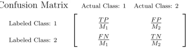
Estimates of class-conditional probabilities may be formed by dividing each element of a class-specific column in the contingency matrix by the total number of classified exemplars from that class. With M1 and M2 exemplars from Classes 1 and 2,

respectively, undergoing classification, we may estimate the class-conditional probabilities from Table 1, as shown in Table 2.

Table 2: Two-Class Confusion Matrix.

 

Confusion Matrix Actual Class: 1 Actual Class: 2

Labeled Class: 1 T P M1 F P M2 Labeled Class: 2 F N M1 T N M2  

The result is a transpose stochastic confusion matrix, such that the sum of each column is one. It is worth mentioning that some authors prefer the proper stochastic presentation, but for the purposes of this thesis, the transpose stochastic is more convenient [6, pp. 8-9]. Also, the term “confusion matrix” sometimes means the

contingency matrix denoted above, and a normalized form of the contingency matrix as illustrated above (that which we term a confusion matrix) may be specified as a “confusion rate matrix” or “confusion ratio matrix” to avoid confusion with the non-normalized

form [8, p. 3], [9, p. 2]. Due to its transpose stochastic nature, the information contained in a 2×2 confusion matrix of this type may be presented as a coordinate pair comprised of one entry from each column, which may then be plotted on a unit square [30, pp. 26-28].

(26)

Assumption 2 (Acceptable Class-Conditional Probability Estimates). Without regard to the method of obtaining an estimate Qc_A of the conditional probability matrix Q_A for a given classification system A, assume that adequate estimation procedures have occurred, such that for all practical purposes, considering Qc_A approximately equal to the matrix

E[Q_A] of expected values of the elements of Qc_A results in no appreciable error; i.e., we may substitute E[Q_A] ≈ Qc_A whenever it is convenient to do so.

Definition 18 (ROC Manifold, ROC Curve). Given an n-class classification problem, the

convex hull of a continuous collection of ROC vectors estimates plotted in

(n2₋_{n)-dimensional space is often termed a ROC curve (for a two-class scenario) or a} ROC manifold [30]. The ROC Convex Hull is abbreviated ROCCH.

If constructing the ROCCH was simple, then comparing only classification systems whose points lie on hull might save time, since no points within the hull interior could possibly represent classification systems superior to those on the hull under any

circumstances [24], [30]. Such considerations would reduce the number of classification systems to compare and contrast; however, since the simplicity of ROCCH calculation, and thus the amount of time to be possibly saved, is questionable, the method of comparison would seem to be far more important than saving time during such a comparison,

depending, of course, on the possible applications of the classification system. Except for time-saving purposes, such geometrical concepts have limited utility under

decision-theoretical constructs, yet the ROCCH, especially in its binary form as the ROC curve, has played a huge role in ROC analysis for many years, and are therefor worthy of mention; however, they are not actually necessary considerations within the framework of risk calculation; therefore, this thesis will refer to them only as auxiliary concepts.

(27)

Definition 19 (Cost Matrix). A cost matrix given by [C]ij = ci|j is an n×n matrix of real numbers representing costs or losses ci|j specific to events

³

e∈ A♮£_{_ℓ

i}¤ ¯¯¯ e∈ Ej

´

, i.e., classification system A assigns label ℓi to an elementary event e when it is actually an element of class Ej, whose class-conditional probability holds the exact same

(i, j)-position in the conditional probability matrix hQ_Ai

ij = qi|j

¡

A¢. These costs may be positive or negative, but most often, the sum of off-diagonal entries in any column isgreater than the diagonal entry itself, indicating that it is better (i.e., less costly) to classify

something as what it actually is rather than anything else [5, pp. 24-25]. This matrix may also be called a “payoff” matrix, so its meaning is almost completely subjective [6, p. 16]. One common form is the so-called “zero-one” transpose stochastic cost matrix, with all zeroes on the diagonal and each column summing to one; however, it is not necessary to restrict the cost matrix to such a form [5, p. 26], [32, p. 7].

Assumption 3 (Fixed Costs). All elements of a given cost matrix C _{are fixed.}

This is a necessary assumption, because costs often are the result of human reasoning, which is very unpredictable; therefore, it is easier to simply choose different possible cost regimes and perform risk calculations under each scenario.

Assumption 4 (Independence of Class-Conditional Costs and Probabilities). Given an

n-class classification system A and any index pairs (i,j), i,j = 1, . . . ,n and (h,k), h,k = 1, . . . ,n, the set nqi|j(A),ch|k

o

consisting of any class-conditional probability qi|j(A), and any cost ch|k, is independent.

Since costs are subjectively defined, it may be possible to envision a scenario where the likelihood of making a particular type of classification decision has a direct impact on the cost of such decision; however, it should therefore also be possible to define scenarios

(28)

where costs do not change as estimates of ROC information change.

Definition 20 (Prevalence Matrix). Given an set ©pjªn_{j = 1} of class prevalences for a classification system A, the prevalence matrix P is an n×n stochastic matrix with each row the same ordered n-tuple pT _{consisting of the class prevalences} ©_pjªn

j = 1: p ≡         p1 ... pn         n×1 =⇒ P=         pT ... pT         n×n =         p1 . . . pn ... p1 . . . pn         n×n (6)

Assumption 5 (Independence of Class Prevalence and Class-Conditional Costs). Given an

n-class classification system A, any index pair (i,j), i,j = 1, . . . ,n, and any index k = 1, . . . ,n, the set ©ci|j,pk

ª

consisting of any cost ci|j and any prior class probability pk, is independent.

Since the definition of cost is purely subjective, it is certainly possible that the individual costs of making classification decisions may be independent of the class

prevalences. For example, in signal detection, this might be like assuming that it is always equally costly to assume an instance of electromagnetic radiation contains noise alone, given that it actually contains a signal, since the binary nature of the setup seems to imply that there is potentially valuable information contained in any type of signal.

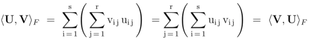
Definition 21 (Matrix Hadamard Product). Given any two matrices U and V of the

same size, the binary Hadamard Matrix Operator ⊙ forms a new matrix U⊙V of the same size. A typical element of the resultant matrix is given by:

(29)

Definition 22 (Frobenius Dot Product). Given any two matrices U and V of size s×r, the Matrix Dot Product Operator h , i_F performs the following reflexive binary operation:

hU,ViF = s X i = 1 Ã _r X j = 1 vi jui j ! = r X j = 1 Ã _s X i = 1 ui jvi j ! = hV,UiF (8)

which is simply the sum of all elements of the Hadamard Matrix Product U⊙V.

Definition 23 (Standard m-Simplex). Given any positive integer m, along with any

ordered m-tuple p∈[0,1]m of non-negative real variables pj, j = 1,2,3, . . . ,m, the standard m-simplex ∆m is the set [3, p. 568], [20, pp. 149-150]:

∆m = ( p∈[0,1]m : m X j = 1 pj ≤ 1 ) (9)

Figure 1 shows an example of how , for a three-class scenario, a two-dimensional prevalence vector p = ¡p1,p2¢ whose coordinates sum to a number less than 1 may be drawn from ∆2. Note that the unspecified value of p3 is found from the conjunctive equation

3

X

j = 1

pj = 1, as illustrated in Figure 2, where this point lies on the tilted surface of a standard 3-simplex.

Definition 24 ( s×r Random Matrix). Given an s×r matrix B = £Bij¤ of event sets

and an s×r matrix X of functions xij defined on Bij, respectively, X is an s×r matrix of random variables, or a random matrix, when the codomain of each function

xij: Bij −→R is the set R of real numbers [33, p. 73].

There is no stipulation as to what type of event set a random variable may be defined upon; therefore, any or all of the event sets in a matrix B of event sets may be either

(30)

0 1/5 1 0 1/5 1

p

1

p

2 ¡1 5, 1 5 ¢ = (p1,p2)

P

2 i=1

(p

i

)

≤

1

Figure 1: ∆2 ≡ ( p ∈ [0,1]2 _: 2 X j = 1 pj ≤ 1 ) . 0 _1/5 1 0 1/5 1 0 3/5 1

p

2

p

1 ¡1 5, 1 5, 3 5 ¢

p

3 Figure 2: ∆3 ≡ ( p ∈ [0,1]3 _: 3 X j = 1 pj ≤ 1 ) .

discrete or continuous. Given an n-class classification system A and the corresponding real-valued matrices Q_A, C, and P introduced in Definitions 17, 19, and 20 above, respectively, note that each is a random matrix defined on a matrix of event sets.

(31)

With regard to the matrices Q_A and P, it is also evident that there are exactly n random variables that are functions of only (n−1) of the random variables inhabiting the same column or row, due to the respective transpose stochastic and stochastic natures of these matrices. For example, since the prevalence matrix P is simply the same random vector p arrayed next to itself n times, the definitions of all n of these functionally dependent variables are exactly the same; similarly, of the remaining (n2₋_{n) random} variables that could be non-constant, there are actually only (n−1) unique random

variables. It will become apparent later why this notation is used; it is sufficient for now to notice that any joint distribution defined for P will be a function of the same (n−1) unique random variables that populate each of its rows, as will any joint distribution defined for a given column of Q_A. The respective stochastic and transpose stochastic natures of these matrices means that an entire row or column vector of random variables will be jointly distributed over a standard (n−1)-simplex (see Definition 23 above), since, for example, the nth _{entry pj} _{randomly drawn in each row vector} _p _{in the prevalence} matrix P is a function pn = 1−

n−1

X

j = 1

pj of the other (n−1) random variables in the row which are randomly drawn before it.

1.3 Problem Statement

Before proceeding further, let us motivate the need for the preceding definitions by means of the following situation. Imagine a stockbroker analyzing the contents of a certain client’s portfolio, implementing an algorithm that classifies stocks as either buy,sell, or hold. Although unknown to the broker or the directors of the corporations whose stocks she analyzes, there are a set of seemingly insignificant factors that, when occurring

(32)

simultaneously, create severe danger of financial ruin for many of these corporations. Her classification system was created to detect just such problems, however, and it reports that 85% of stocks in this particular portfolio are sell stocks—i.e., stocks that ought to be sold immediately. Since the broker has never seen numbers for the sell class greater than 10%, she begins to question the results, and therefore does not immediately sell those stocks. Time ticks by, and it becomes more readily apparent to the corporations and the broker that the stocks are highly over-valued, and the window of opportunity to sell with minimal loss shrinks away overnight.

If the broker in this case had been informed beforehand that the classification system she used had been selected and tuned specifically to the cost structure dictated by her management, and that the distribution of stock class prevalences provided for the

possibility of unknown factors causing a change in stock class prevalences, she might have had more confidence in the classification system, and then acted immediately to avoid losing more money for her client, because her risk was already minimized by acting on the results of the classification system.

Although the scenario above might be unrealistic, there are many classification situations which entail potentially much greater costs, e.g., from the loss of life (military applications are just one). However, many popular methods of comparing classification systems to one another do not consider the whole picture of risk—i.e., the costs and class prevalences in addition to an estimate of the class-conditional probabilities. In addition to these oversights, and due to the fact that volume under a ROC surface (VUS) in a

three-class case would have six dimensions, visualization of geometric surfaces becomes impossible, so ignoring more than just one of the entries per column of a conditional

(33)

probability matrix estimate is also sometimes chosen as an alternative [21]. Most attempts to generalize geometric concepts to the general n-class case choose to ignore either the class prevalences or the costs [7], [9], [35]. If Assumptions 1, 2, 3, 4, and 5 are relatively safe assumptions to make, then the concept of risk offers the opportunity a much more robust form of ROC analysis; i.e., one which considers many more of the characteristics of the operating environment in which the receiver of information resides.

(34)

II. Review of Related ROC Analysis Topics

The monograph by Egan serves as a starting point for modern binary ROC analysis. It contains much of the terminology and geometry still in use today, as well as a framework for risk calculations [6, p. 16]. Based on his work, for a given classification system A and accompanying conditional probability, cost, and prevalence matrices Q_A, C, and Pas given in Definitions 9, 17, 19, and 20 of Chapter I, respectively, we define the risk R(A) of a classification system A (suppressing notational dependence on A) as :

R = DQ,¡C⊙P¢E

F (10)

with Matrix Hadamard Product ⊙ and Frobenius Dot Product h,iF as defined in

Chapter I, Definitions 21 and 22, respectively. Egan notes that (10) gives the expected cost over a sufficiently large number of trials; therefore, from this point onward, we shall

assume, as in Chapter I, Assumption 2, that such is the case [6, pp. 16-17].

2.1 Two-Class ROC Analysis

Assume the following notation of a transpose stochastic confusion matrix for some binary classification system A (again, suppressing notational dependence on A):

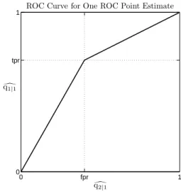
    d q1|1 qd1|2 d q2|1 qd2|2     =     tpr f pr f nr tnr     (11)

(35)

negative or non-target class, thereby leading to the abbreviations for true positive rate (tpr), false negative rate (fnr), false positive rate (fpr), and true negative rate (tnr) in common use today [10], [32]. Since this matrix is transpose stochastic, its information may be represented by only one entry from each column. Although there are four possible ways to do this, the common way is to plot (f pr, tpr) as in Figure 3, so that the coordinate representation of a perfect classifier is at (0,1). In this coordinate system, maximal area beneath the lines connecting a plotted point for a given classification system to the corners (0,0) and (1,1) is seen as desirable [8, pp. 108-110].

Based on this geometrical frame of reference, one of the most popular means of evaluating classification system effectiveness is by the Area Under the ROC Curve (AUC) performance measure, which calculates geometrically the area under the convex hull of a collection of ROC vector estimates plotted in this way to represent a family of binary classification systems [10], [13], [26]. Instead of analyzingcollections of ROC vectors, consider the case with just one plotted ROC vector [8, pp. 108-110], as in Figure 3.

0 fpr 1

0 tpr

1 ROC Curve for One ROC Point Estimate

d

q2|1 d

q1|1

Figure 3: ROC Curve for One ROC Point Estimate.

(36)

AUC = (1−f pr)(tpr) + (f pr)(tpr) 2 + (1−f pr)(1−tpr) 2 = £ 2(1−f pr)(tpr)¤ + £(f pr)(tpr)¤ + £(1−f pr)(1−tpr)¤ 2 = 2 £ tpr − (f pr)(tpr)¤ + (f pr)(tpr) + 1 − tpr − f pr + (tpr)(f pr) 2 = 2(tpr) − 2(f pr)(tpr) + (f pr)(tpr) + 1 − tpr − f pr + (tpr)(f pr) 2 = tpr + (1 − f pr) 2 = tpr + tnr 2 (12)

where the last observation is made possible by the conjunctive equation f pr + tnr = 1 pertaining to the left columns in (11) above. Now, if we assume equal class prevalences

M1 = M = M2 we may write: AUC = tpr + tnr 2 ≡ T P M1 + T N M2 2 = T P M + T N M 2 = T P + T N 2M = T P + T N M1 + M2 ≡ Accuracy (13)

Accuracy is related to risk through the AUC, as seen when we calculate the approximate risk R ≈ DQb ,¡C⊙P¢E

F (per Assumption 2, Chapter I) indicated by (10) for a zero-one cost matrix C = h 0 1_{1 0} i under equal class prevalences:

(37)

R ≈DQb ,¡C⊙P¢E F = *" tpr f pr f nr tnr # , Ã" 0 1 1 0 # ⊙ " 1 2 1 2 1 2 1 2 #!+ F = *" tpr f pr f nr tnr # , " 0 1₂ 1 2 0 #+ F = (0 + f pr) + (f nr + 0) 2 = (1 − tnr) + (1 − tpr) 2 = 1 − tpr + tnr 2 = 1 − AUC (14)

where the last relation again is made possible by the conjunctive equations from (11) above; therefore, by (12) above, the risk R for a zero-one cost matrix and equal class prevalences is simply (1 − Accuracy) under the same assumptions, and (1 − AUC) in general for a ROC curve with only one point. It is interesting to note that if the coordinate pair used to represent the information of the transpose stochastic matrices in (11) were (f pr, f nr) instead of (f pr, tpr) , the calculation in (14) would yield R ≈ AUC.

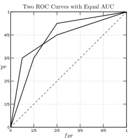
Neither the AUC nor Accuracy consider costs, but unlike Accuracy, the AUC also does not consider class prevalences in its calculation, and so the AUCs for two very different classification systems may be equal, as shown in Figure 4.

There is some merit to the idea that the conventional formula for Accuracy considers class prevalences, but it still ignores the costs, and for that reason is incomplete as a measure of risk [10], [14], [19], [25]. It is also not robust to changes in class prevalences when extended to a classification system with more than 2 classes. There are quite a few other performance measures related to Accuracy or the AUC which we shall not mention,

(38)

0 1/5 2/5 3/5 4/5 1 0 1/5 2/5 3/5 4/5

1 Two ROC Curves with Equal AUC

f pr tpr

Figure 4: Two ROC Curves with Equal AUC.

due to the similarity of their weaknesses to changes in class prevalences and differing costs. Proceeding in this manner, it becomes apparent that any other ROC analysis calculation based on Accuracy or the AUC is equivalent to a risk calculation with certain restrictions on the values of the cost and prior information.

In general, it appears that none of the binary ROC analysis methods in popular use today truly utilize the significant Bayesian inputs of costs and prior probabilities.

2.2 Multi-Class ROC Analysis

Extending classical ROC analysis beyond the realm of binary classification is difficult. Some authors have proposed using only one entry per column of a 3×3 transpose

stochastic confusion matrix, eliminating most of the ROC information, and explicitly considering neither costs nor class prevalences in their calculations [21, pp. 80-82], [22, p. 3441] [34, p. 4]. More recent approaches consider either the costsor the priors as one of the parameters in the threshold set, ignoring the effect of the other, or suggest plotting different curves for each pair of classes as done in binary ROC analysis [9], [12], [36].

(39)

Due to the conjunctive equations accompanying any conditional probability matrix, the Volume Under the Surface (VUS) for an n-class scenario is only a true extension of the AUC when it is (n2₋_{n)-dimensional, however, some authors, in order to produce visible} surfaces, plot only a 3-dimensional surface for a 3-class system [4], [21], [22]. Some, who realize the weakness such a scheme entails, allude to the calculation of risk; however, the calculation is not performed, because, for example, the need to assume unknown costs is deemed important. In general, breaching Assumptions 1, 2, 3, 4, and 5 from Chapter I is never mentioned as a cause for not calculating the risk [8], [9].

2.3 Need for a ROC Risk Functional

The world of classical ROC analysis seems to be stuck unnecessarily in a frame of reference that considers geometrical analyses as the gold standard of ROC analysis methods, when in fact, if Assumptions 1, 2, 3, 4, and 5 from Chapter I can be met, the comparison of classification systems by risk comparison is not simpler and more

comprehensive. In addition, risk-based comparison of classification systems falls closer to the reach of the ordinary decision-maker, who is usually not involved in obtaining estimates of class-conditional probabilities, but usually is responsible for defining costs and may even have some knowledge of class prevalence distributions. When risk-based comparisons of classification systems are implemented, the result is much simpler, as well as more considerate of the crucial role of both costs and class prevalences in ROC analysis [32].

(40)

III. Development and Definition of the ROC Risk Functional

The ROC Functional f_A suggested in [31] and [32] for a family A _{of classification systems}

is a ROC analysis method which minimizes risk. Additionally, it was proposed in [32] to allow the Hadamard Product ˆγγγ = ¡c⊙p¢ of vectors of costs and class prevalences, constructed in a particular way, to vary over a range Γ = {γγγ:γγγ = c⊙p}, along with restrictions on cost. This Robust Functional implicitly incorporated Assumptions 1, 2, and 4 from Chapter I, but did not incorporate Assumptions 3 and 5 from that Chapter, which made the problem more difficult. The equation was written as:

R¡fA,Γ ¢ = min q∈Q Z Γ hq,γγγbiW(γγγ)dγγγ (15)

where Q is a collection Q = {q: q∈Q} of ROC vectors corresponding to the family A

of classification systems and W(γγγ) is a joint weighting function, of the cost-prior

Hadamard Product vector γγγ_b = c ⊙ _bp, cast either as a probability density function or a belief function [32, p. 6].

In addition to the implicit incorporation of Assumptions 1, 2, and 4 from Chapter I, if we also incorporate Assumptions 3 and 5 from the same Chapter, we may fashion the distributions of costs and priors independently from one another by making over q, c, and

p in (15) above to be the random matrices Q_A, C, and P (see Definitions 24, 17, 19, and 20 from Chapter I). Without explicitly denoting dependence on the classification system

A, we define marginal weighting functions WQ(Q), WC(C), and WP(P). Since these

marginal distributions are defined for sets of random variables assumed independent from one another, they satisfy the separability condition [33, p. 245]:

(41)

WQ,C,P(Q,C,P) = WQ(Q)WC(C)WP(P)

We shall now examine possible joint probability density functions WP(P) on the priors such that the constraints of the conjunctive equation

n

X

j = 1

pj = 1 are met.

Note that (15) simply calculates Bayes risk, or the expected value of Equation (10), Chapter II. Without explicitly denoting dependence on the classification system A or functional dependence on the variables in the matrices Q_A, C, and P, we may write:

(42)

where the boldface expected value E£·¤ denotes amatrix £E(·)¤_ij of expected values, and where we have introduced the notation of integration with respect to a matrix, such that

R

[·] dX denotes the multiple integration operator:

Z . . . . Z . . . Z Z [·] dx11dx12 . . . dx1r . . . dxsr

with respect to all of the variables in the matrix X of size s×r, such that dX denotes the product of all differential elements dxij of variables in X, ∀ i∈ {1,2,3, . . . ,s} and j∈ {1,2,3, . . . ,r}. Note that without Assumptions 1, 2, 3, 4, and 5 from Chapter I, we could not perform this simple dot product calculation for Bayes risk [33, p. 233-246].

3.1 Definition of the ROC Risk Functional Given a family A_Θ ₌ _{_A

θ: θ ∈Θ} of n-class classification systems of form

Aθ: E−→L over a threshold set Θ, with common cost and prevalence matrices C and P and a collection nQ_Aθ:θ ∈Θ

o

of conditional probability matrices, as defined in Chapter I, Definitions 11, 10, 19, 20, and 17, respectively, define the ROC Risk Functional (RRF) as a threshold parameter θ∈Θ such that the classification system Aθ minimizes Bayes risk over the family A_Θ _{of classification systems:}

arg min Aθ∈AΘ n E£RAθ ¤o ≡ arg min Aθ∈AΘ ( E· DQ_A_θ , (C⊙P)E F ¸) ≈ arg min Aθ∈AΘ ½D d Q_A_θ , C⊙E[P]E F ¾ (17)

As a result of Assumptions 1, 2, 3, 4, and 5 from Chapter I, expected values for elements of the cost, prevalence, and conditional probability matrices may all be analyzed

(43)

and estimated independently of elements of any other matrix appearing in (17), prior to using them in calculation of Bayes’ risk when employing the RRF.

We now consider the effect on E[P] of varying our assumptions on P. These

assumptions may take many different forms. For example, we may simply consider that we already have an acceptable estimate of P, and treat it as a constant, bringing us back to a form like that of Equation (10), Chapter II. We may also populate its rows with the

transpose mean vector of a joint statistical distribution, such as a joint uniform distribution representing no knowledge of prior probabilities, or some other jointly continuous

fixed-support probability distribution function, such as a multivariate Beta distribution. Finally, we may simply impose a joint weighting based on expert knowledge and belief (a.k.a., a belief function, which is actually a more general type of weighting than a probability distribution function, with potentially greater utility for actual end-users of classification systems [28, pp. 38-39]. In the latter case, we do not end up with a classical risk, but rather a fuzzy risk. Since the case where all random variables in the prevalence matrix P are constants is a matter of simple algebra, we shall examine a small sampling of more interesting possibilities.

3.2 Completely Unknown Class Prevalences

As noted in Chapter I, for an n-class classification system, exactly (n−1) of the class prevalences are distributed over a standard (n−1)-simplex, and the remaining class prevalence is found by solving the conjunctive equation inherent in each row of the stochastic matrix P of class prevalences. Observing Theorem 2, Appendix A:

(44)

m! = _R 1 1 0 R1−p1 0 R1−p1−p2 0 . . . R1−Pm−1 j = 1(pj) 0 dpm . . . dp3dp2dp1 (18)

we see the integral in the denominator of (18) is simply over the standard m-simplex ∆m⊂[0,1]m _{(see Definition 23, Chapter I). Apply this observation and (18) to the} standard simplex ∆n−1 from which the first (n−1) class prevalences are drawn, yielding:

Z ∆n−1 dpn−1. . . dp1 = Z 1 0 Z 1−p1 0 Z 1−p1−p2 0 . . . Z 1−Pn−2 j = 1(pj) 0 dpn−1. . . dp3dp2dp1 = 1 (n−1)! (19)

Assuming nothing whatsoever is known about the prior probabilities, a jointly continuous uniform probability density function WP,uniform(p1, . . . ,pn−1) of (n−1) class

prevalences over the standard (n−1)-simplex, satisfying

R ∆n−1 WP,uniform ¡ p1, . . . ,pn−1 ¢ dpn−1 . . . dp1 = 1 is then given by [3, p. 568]: WP,uniform ¡ p1, . . . ,pn−1 ¢ =        (n−1)!, ¡p1, . . . ,pn−1 ¢ ∈ ∆n−1 0, otherwise (20)

If we consider the quantity E[P] appearing in (17) above to be the matrix of expected values whose typical element is:

" Z ∆n−1 pijWPj,uniform ¡ p1j, . . . ,pn−1,j ¢ dpn−1,j. . . dp1j # ij

(45)

that all entries in a given row i, save pin = Ã 1− n−1 X j = 1 pij !

, are the class prevalences

©

pij

ªn−1

j=1, for all rows i = 1,2,3 . . . ,n. Also, since the rows are identical, there is no need to keep the subscript i when referring to a prior probability pj for class E_j.

It iscrucial to state here that even though we use the wordsfirst and last to describe the class prevalences, the order in which the so-called first (n−1) class prevalences are randomly drawn from their joint distribution has nothing to do with the ordering of the index set Λ by which we link them to elements of the label set.

Since pn = 1− n−1

X

j = 1

pj is a function of the (n−1) class prevalences whose joint distribution is WP,uniform(p1, . . . ,pn−1), we may use the weighting in (20) to calculate an

expected value E¡pn¢, using some of the equation patterns seen in the proof of Theorem 2, Appendix A: E¡pn¢ = E Ã 1− n−1 X j = 1 pj ! = Z ∆n−1 Ã 1− n−1 X j = 1 pj ! WP ¡ p1 . . .pn−1 ¢ dpn−1, . . . , dp1 = Z ∆n−1 Ã 1− n−1 X j = 1 pj ! (n−1)!dpn−1 . . . dp1 = (n−1)! Z ∆n−1 Ã 1− n−1 X j = 1 pj ! dpn−1 . . . dp1 = (n−1)! Z 1 0 Z 1−p1 0 . . . Z 1−Pn−2 j=1 (pj) 0 µ 1− n−1 X j=1 pj ¶ dpn−1 . . . dp2dp1 = (n−1)! µ 1 n! ¶

, by (28) and (29), Theorem 2 proof, Appendix A

= 1

n

(46)

We may calculate expected values for the other (n−1) class prevalences in a row by means of Corollary 1, Appendix A, which is known to be true for positive integers less than 48 (i.e., for most practical classification purposes):

(m + 1)! = _R 1 1 0 R1−p1 0 R1−p1−p2 0 . . . RPm−1 i = 1(pi) 0 pj dpm . . . dp3dp2dp1 ≡ R 1 ∆m pjdppp , ∀ j = 1,2,3, . . . ,m (22)

Apply (22) to each of the expected values E¡pj¢, j = 1, . . . ,n−1:

E¡pj ¢ = Z ∆n−1 pjWP ¡ p1, . . . ,pn−1 ¢ dpn−1 . . . dp1 = Z ∆n−1 pj(n−1)!dpn−1 . . . dp1 = (n−1)! Z ∆n−1 pj dpn−1 . . . dp1 = (n−1)! µ 1 n! ¶ = 1 n, ∀ j = 1, . . . ,n−1 (23)

so by (21), each entry in the n×n matrix E£P_A¤ is exactly _n1; therefore, if we set all class prevalences equal to begin with, the resultant expected value matrix is the same as when we assume an underlying multivariate uniform distribution over ∆n−1.

3.3 Limited Knowledge of Class Prevalences

Probability density functions, such as the multivariate uniform and Beta

distributions, are only a specific kind of “weighting” function WP to be used in evidential

(47)

probability is only a specific instance of an infinite number of ways to approach the so-called “doctrine of chances” [2], [28]. This is the reason we have chosen to denote the weighting function as WP instead of the usual symbol fP for a marginal probability density function

of the class prevalences. Even though we leave the framework open for expansion, we will only consider one additional classical distribution—a multivariate general Beta.

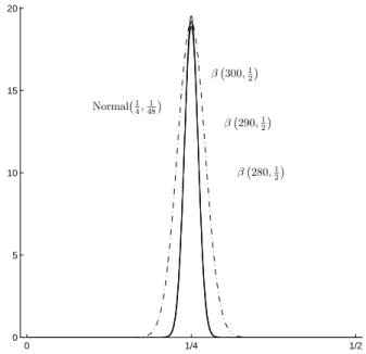
The marginal versions of a general Beta distribution are very flexible and may even be made to approximate normal distributions over limited support intervals. The standard univariate Beta distribution has support on [0,1], and thus has a set of two parameters (for shape), but the general form has four parameters, because it includes two parameters Slower and Supper giving the bounds of the support interval [lower, upper]⊂R _{over which it is}

defined [15, p. 210]. In this thesis we shall always define the lower support bound to be

lower = 0, effectively reducing the number of parameters to three; further, we shall also consider only those marginal Beta distributions that have the potential to approximate a normal distribution with a mean of ¡upper₂ ¢ over their support intervals; i.e., those

symmetric about the midpoint of their support. This means the two shape parameters are equal, so we have reduced the total number of possibly unique parameters to two—one for shape, and one for support. We shall denote this special case of the general Beta

distribution as β(t, S), where t is the value of the common shape parameter, and S is the upper bound of the support interval [0, S]. In the case where a joint probability density function WP,β is defined over a standard simplex ∆m, we shall indicate such joint support by the notation β(t,∆m), where t∈(0,∞)m is a vector of the common shape parameters used in the symmetric marginal probability density functions.

(48)

prevalences randomly drawn over an (n−1)-simplex is a function of all prevalences previously drawn. In fact, it is because of this that expected value calculations for any function f¡p1, . . . ,pn−1

¢

may then be performed by means of the operator:

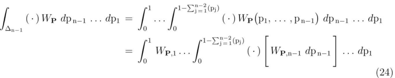
Z ∆n−1 (·)WP dpn−1 . . . dp1 = Z 1 0 . . . Z 1−Pn−2 j = 1(pj) 0 (·)WP ¡ p1, . . . ,pn−1 ¢ dpn−1 . . . dp1 = Z 1 0 WP,1. . . Z 1−Pn−2 j = 1(pj) 0 (·) " WP,n−1 dpn−1 # . . . dp1 (24) by decomposing the joint distribution WP

¡

p1, . . . ,pn−1

¢

into a form allowing elimination of one variable at a time, working from the inside of the integral toward the outside:

WP ¡ p1, . . . ,pn−1 ¢ = hWP,1 ¡ p1¢i hWP,2 ¡ p1,p2¢i. . . hWP,n−1 ¡ p1, . . . ,pn−1 ¢i (25)

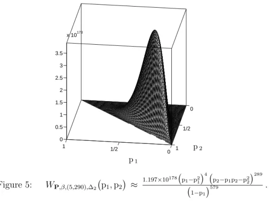
Considering a 3-class scenario, we attempt to approximate a bivariate normal

distribution of the first two class prevalences randomly drawn from the standard 2-simplex. Figure 5 depicts a bivariate β¡[5,290],∆2¢ probability distribution function

WP,β,(5,290),∆2

¡

p1,p2

¢

of two class prevalences over the standard 2-simplex. The values of the common shape parameters for the marginal probability density functions were chosen after examining Figures 6 and 7.

(49)

0 1/2 1 0 1/2 1 0 0.5 1 1.5 2 2.5 3 3.5 x 10173 p2 p1 Figure 5: WP,β,(5,290),∆2 ¡ p1,p2¢ ≈ 1.197×10178 ¡ p1−p2₁ ¢4¡ p2−p1p2−p2₂ ¢289 ¡ 1−p1 ¢579 . 0 1/2 1 0 1 2 3 Normal¡1 2, 1 6 ¢ β(3,1) β(4,1) β(5,1)

(50)

0 1/4 1/2 0 5 10 15 20 Normal¡1 4, 1 48 ¢ β¡280,1 2 ¢ β¡290,1 2 ¢ β¡300,1 2 ¢

(51)

IV. Application of Results to Actual Data

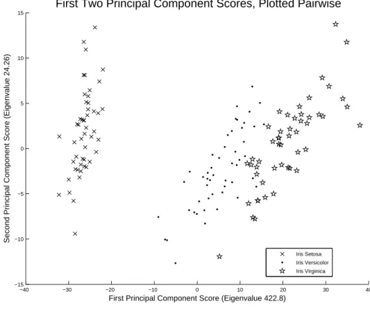
The Fisher Iris Data is a well-known data set consisting of four measurements (in

millimeters) of various physical attributes for three subspecies of iris flowers—namely, Iris Setosa, Iris Versicolor, and Iris Virginica. There are 50 such sets of measurements per species, allowing for great flexibility when varying class distributions such that the data set is always of significant size. Principal components analysis (PCA) of the data reveals that the first two principal components account for about 98% of the variance in the data; therefore, we sped up computation by only using the component scores from these two components. The PCA scores for these two components are shown in Figure 8.

−40 −30 −20 −10 0 10 20 30 40 −15 −10 −5 0 5 10 15

First Principal Component Score (Eigenvalue 422.8)

Second Principal Component Score (Eigenvalue 24.26)

First Two Principal Component Scores, Plotted Pairwise

Iris Setosa Iris Versicolor Iris Virginica

Figure 8: First Two Principal Component Scores, Fisher Iris Data.

(52)

amongst the classes according to a set of three positive numbers summing to 1, the first two of which were drawn from a specific bivariate distribution assumed to exist over the standard 2-simplex, rounding determining the actual prevalence, which may not be exactly equal to the goal prevalence actually drawn due to the fact that one cannot classify a partial exemplar. We cast Iris Setosa as Class 1, Iris Versicolor as Class 2, Iris Virginica as Class 3, applying the uniform and symmetric Beta distributions examined in Chapter III, Sections 3.2 and 3.3 to the PCA score data to test the validity of Assumption 1 from Chapter I, while comparing the performance of the ROC Risk Functional (RRF) to Accuracy.

To test the validity of Assumption 1 from Chapter I, we used the non-parametric Kendall’s Tau Correlation Coefficient statistical test, with a null hypothesis of no

dependence between a class-conditional probability estimate q_ci|j and the prevalence pj of the class E_j _{upon which it is conditioned [11, pp. 404-405]. Note that we assumed it}

sufficient to test only between a conditional probability estimate qi\|j

¡ Aθ

¢

and the prevalence pj of the class upon which it is conditioned, since the class prevalence pj actually appears in the formulas for qi|j, ∀ i = 1, . . . ,n (see Definition 16, Chapter I).

Under this assumption, nine separate Kendall’s Tau tests were performed after each set of 37 replicates, testing for independence between each of the 9 sets of 37 class-conditional probabilities and a similar population of actual class prevalences for the class upon which they are conditioned, reporting the mean absolute value of Kendall’s Tau Correlation Coefficients and corresponding mean p-values from those tests in a pair of 9×9 matrices.

A Monte Carlo simulated power analysis algorithm provided a 99% confidence interval of (0.8083,0.8282) for the power of a test with 37 sample points and an