Bayesian Time Series Learning with Gaussian Processes

with Gaussian Processes

Roger Frigola-Alcalde

Department of Engineering

St Edmund’s College

University of Cambridge

August 2015

This dissertation is submitted for the degree of Doctor of Philosophy

as the social sciences, biology, engineering or econometrics. In this dissertation, we present a number of algorithms designed to learn Bayesian nonparametric models of time series. The goal of these kinds of models is twofold. First, they aim at making predictions which quantify the uncertainty due to limitations in the quantity and the quality of the data. Second, they are flexible enough to model highly complex data whilst preventing overfitting when the data does not warrant complex models.

We begin with a unifying literature review on time series mod-els based on Gaussian processes. Then, we centre our attention on the Gaussian Process State-Space Model (GP-SSM): a Bayesian nonparametric generalisation of discrete-time nonlinear state-space models. We present a novel formulation of the GP-SSM that offers new insights into its properties. We then proceed to exploit those insights by developing new learning algorithms for the GP-SSM based on particle Markov chain Monte Carlo and variational infer-ence.

Finally, we present a filtered nonlinear auto-regressive model with a simple, robust and fast learning algorithm that makes it well suited to its application by non-experts on large datasets. Its main advan-tage is that it avoids the computationally expensive (and potentially difficult to tune) smoothing step that is a key part of learning non-linear state-space models.

cepting a candidate for a PhD in statistical machine learning who barely knew what a probability distribution was. I am also grateful to Zoubin Ghahramani, Rich Turner and Daniel Wolpert for creat-ing such a wonderful academic environment at the Computational and Biological Learning Lab in Cambridge; it has been incredible to interact with so many talented people. I would also like to thank Thomas Sch ¨on for hosting my fruitful academic visit at Link ¨oping University (Sweden).

I am indebted to my talented collaborators Fredrik Lindsten and Yutian Chen. Their technical skills have been instrumental to de-velop ideas that were only fuzzy in my head.

I would also like to thank my thesis examiners, Rich Turner and James Hensman, and Thang Bui for their helpful feedback that has certainly improved the thesis. Of course, any remaining inaccura-cies and errors are entirely my fault!

Finally, I can not thank enough all the colleagues, friends and fam-ily with whom I have spent so many joyful times throughout my life.

D

ECLARATION

This dissertation is the result of my own work and includes noth-ing which is the outcome of work done in collaboration except as specified in the text.

This dissertation is not substantially the same as any that I have submitted, or, is being concurrently submitted for a degree or diplo-ma or other qualification at the University of Cambridge or any other University or similar institution. I further state that no sub-stantial part of my dissertation has already been submitted, or, is being concurrently submitted for any such degree, diploma or other qualification at the University of Cambridge or any other Univer-sity of similar institution.

This dissertation does not exceed 65,000 words, including appen-dices, bibliography, footnotes, tables and equations. This disserta-tion does not contain more than 150 figures.

Cat.

“I don’t much care where —” said Alice.

“Then it doesn’t matter which way you go,” said the Cat. “— so long as I getsomewhere,” Alice added as an explanation. “Oh, you’re sure to do that,” said the Cat, “if you only walk long enough.”

1 Introduction 1

1.1 Time Series Models . . . 1

1.2 Bayesian Nonparametric Time Series Models . . . 2

1.2.1 Bayesian Methods . . . 2

1.2.2 Bayesian Methods in System Identification . . . 4

1.2.3 Nonparametric Models . . . 4

1.3 Contributions . . . 5

2 Time Series Modelling with Gaussian Processes 7 2.1 Introduction . . . 7

2.2 Gaussian Processes . . . 8

2.2.1 Gaussian Processes for Regression . . . 9

2.2.2 Graphical Models of Gaussian Processes . . . 11

2.3 A Zoo of GP-Based Dynamical System Models . . . 12

2.3.1 Linear-Gaussian Time Series Model . . . 13

2.3.2 Nonlinear Auto-Regressive Model with GP . . . 14

2.3.3 State-Space Model with Transition GP . . . 16

2.3.4 State-Space Model with Emission GP . . . 18

2.3.5 State-Space Model with Transition and Emission GPs . . 19

2.3.6 Non-Markovian-State Model with Transition GP . . . 21

2.3.7 GP-LVM with GP on the Latent Variables . . . 22

2.4 Why Gaussian Process State-Space Models? . . . 23

3 Gaussian Process State-Space Models – Description 25 3.1 GP-SSM with State Transition GP . . . 25

3.1.1 An Important Remark . . . 28

3.1.2 Marginalisation off1:T . . . 29

3.1.3 Marginalisation off(x) . . . 30

3.2 GP-SSM with Transition and Emission GPs . . . 31

3.2.1 Equivalence between GP-SSMs . . . 32

3.3 Sparse GP-SSMs . . . 33

3.4 Summary of GP-SSM Densities . . . 34

4 Gaussian Process State-Space Models – Monte Carlo Learning 37 4.1 Introduction . . . 37

4.2 Fully Bayesian Learning . . . 38

4.2.1 Sampling State Trajectories with PMCMC . . . 38

4.2.2 Sampling the Hyper-Parameters . . . 40

4.2.3 Making Predictions . . . 41 ix

4.2.4 Experiments . . . 41

4.3 Empirical Bayes . . . 44

4.3.1 Particle Stochastic Approximation EM . . . 45

4.3.2 Making Predictions . . . 47

4.3.3 Experiments . . . 48

4.4 Reducing the Computational Complexity . . . 51

4.4.1 FIC Covariance Function . . . 51

4.4.2 Sequential Construction of Cholesky Factorisations . . . 52

4.5 Conclusions . . . 53

5 Gaussian Process State-Space Models – Variational Learning 55 5.1 Introduction . . . 55

5.2 Evidence Lower Bound of a GP-SSM . . . 56

5.2.1 Interpretation of the Lower Bound . . . 58

5.2.2 Properties of the Lower Bound . . . 59

5.2.3 Are the Inducing Inputs Variational Parameters? . . . 60

5.3 Optimal Variational Distributions . . . 60

5.3.1 Optimal Variational Distribution foru . . . 60

5.3.2 Optimal Variational Distribution forx . . . 61

5.4 Optimising the Evidence Lower Bound . . . 63

5.4.1 Alternative Optimisation Strategy . . . 63

5.5 Making Predictions . . . 64

5.6 Extensions . . . 65

5.6.1 Stochastic Variational Inference . . . 65

5.6.2 Online Learning . . . 66

5.7 Additional Topics . . . 67

5.7.1 Relationship to Regularised Recurrent Neural Networks 67 5.7.2 Variational Learning in Related Models . . . 68

5.7.3 Arbitrary Mean Function Case . . . 71

5.8 Experiments . . . 72

5.8.1 1D Nonlinear System . . . 72

5.8.2 Neural Spike Train Recordings . . . 72

6 Filtered Auto-Regressive Gaussian Process Models 75 6.1 Introduction . . . 75

6.1.1 End-to-End Machine Learning . . . 76

6.1.2 Algorithmic Weakening . . . 76

6.2 The GP-FNARX Model . . . 77

6.2.1 Choice of Preprocessing and Covariance Functions . . . 78

6.3 Optimisation of the Marginal Likelihood . . . 79

6.4 Sparse GPs for Computational Speed . . . 80

6.5 Algorithm . . . 80

6.6 Experiments . . . 81

7 Conclusions 85 7.1 Contributions . . . 85

A Approximate Bayesian Inference 87

A.1 Particle Markov Chain Monte Carlo . . . 87 A.1.1 Particle Gibbs with Ancestor Sampling . . . 87 A.2 Variational Bayes . . . 89

Introduction

”The purpose of computing is insight, not numbers.”

Richard W. Hamming ”The purpose of computing is numbers — specifically, correct numbers.” Leslie F. Greengard

1.1

T

IME

S

ERIES

M

ODELS

Time series data consists of a number of measurements taken over time. For example, a time series dataset could be created by recording power generated by a solar panel, by storing measurements made by sensors on an aircraft, or by monitoring the vital signs of a patient in a hospital. The ubiquity of time series data makes its analysis important for fields as disparate as the social sciences, biology, engineering or econometrics.

Time series tend to exhibit high correlations induced by the temporal struc-ture in the data. It is therefore not surprising that specialised methods for time series analysis have been developed over time. In this thesis we will focus on a model-based approach to time series analysis. Models are mathematical constructions that often correspond to an idealised view about how the data is generated. Models are useful to make predictions about the future and to better understand what was happening while the data was being recorded.

The process of tuning models of time series using data is called system iden-tification in the field of control theory (Ljung, 1999). In the fields of statistics and machine learning it is often referred to as estimation, fitting, inference or learning of time series (Hamilton, 1994; Shumway and Stoffer, 2011; Barber et al., 2011; Tsay, 2013). Creating faithful models given the data at our disposal is of great practical importance. Otherwise any reasoning, prediction or design based on the data could be fatally flawed.

Models are usually not perfect and the data available to us is often limited in quantity and quality. It is therefore normal to ask ourselves: are we limited

to creating just one model or could we make a collection of models that were all plausible given the available data? If we embrace uncertainty, we can move from the notion of having a single model to that of keeping a potentially infinite collection of models and combining them to make decisions of any sort. This is one of the fundamental ideas behind Bayesian inference.

In this thesis, we develop methods for Bayesian inference applied to dy-namical systems using models based on Gaussian processes. Although we will work with verygeneralmodels that can be applied in a variety of situations, our mindset is that of the field of system identification. In other words, we focus on learning models typically found in engineering problems where a relatively limited amount of noisy sensors give a glimpse at the complex dynamics of a system.

1.2

B

AYESIAN

N

ONPARAMETRIC

T

IME

S

ERIES

M

OD

-ELS

1.2.1

B

M

When learning a model from a time series, we never have the luxury of an infinite amount of noiseless data and unlimited computational power. In prac-tice, we deal with finite noisy datasets which lead to uncertainty about what the most appropriate model is given the available data. In Bayesian inference, probabilities are treated as a way to represent the subjective uncertainty of the rational agent performing inference (Jaynes, 2003). This uncertainty is repre-sented as a probability distribution over the model given the data

p(M | D), (1.1)

where the model is understood here in the sense of the functional formand the value of any parameter that the model might have. This contrasts with the most common approaches to time series analysis where asinglemodel of the system is found, usually by optimising a cost function such as the likelihood (Ljung, 1999; Shumway and Stoffer, 2011). After optimisation, the resulting model is consideredthe best available representation of the system and used for any further application.

In a Bayesian approach, however, it is acknowledged that several models (or values of a parameter) can be consistent with the data (Peterka, 1981). In the case of a parametric model, rather than obtaining a single estimate of the “best” value of the parametersθ∗_{, Bayesian inference will produce a posterior}

probability distribution over this parameterp(θ|D). This distribution allows for the fact that several values of the parameter might also be plausible given the observed dataD. The posteriorp(θ|D)can then interpreted as our degree of belief about the value of the parameterθ. Predictions or decisions based on the posterior are made by computing expectations over the posterior. Infor-mally, one can think of predictions as being an average using different values

of the parameters weighted by how much the parameter is consistent with the data. Predictions can be made with error bars that represent both the system’s inherent stochasticityandour own degree of ignorance about what the correct model is.

For the sake of example, let’s consider a parametric model of a discrete-time stochastic dynamical system with a continuous state defined byxt. The state transition density is

p(xt+1|xt, θ). (1.2)

Bayesian learning provides a posterior over the unknown parameter θgiven the datap(θ|D). To make predictions about the state transition we can integrate over the posterior in order to average over all plausible values of the parameter after having seen the data

p(xt+1|xt,D) =

Z

p(xt+1|xt, θ)p(θ|D)dθ. (1.3) Here, predictions are made by considering all plausible values ofθ, not only a “best guess”.

Bayesian inference needs a prior: p(θ)for our example above. The prior is a probability distribution representing our uncertainty about the object to be inferred beforeseeing the data. This requirement of a subjective distribution is often criticised. However, the prior is an opportunity to formalise many of the assumptions that in other methods may be less explicit. MacKay (2003) points out that “you cannot do inference without making assumptions”. In Bayesian inference those assumptions are very clearly specified.

In the context of learning dynamical systems, Isermann and M ¨unchhof (2011) derive maximum likelihood and least squares methods from Bayesian infer-ence. Although maximum likelihood and Bayesian inference are related in their use of probability, there is a fundamental philosophical difference. Spiegel-halter and Rice (2009) summarise it eloquently:

At a simple level, ‘classical’ likelihood-based inference closely resembles Bayesian inference using a flat prior, making the posterior and likelihood proportional. However, this underestimates the deep philosophical differ-ences between Bayesian and frequentist inference; Bayesian [sic] make statements about the relative evidence for parameter values given a dataset, while frequentists compare the relative chance of datasets given a parame-ter value.

Bayesian methods are also relevant in “big data” settings when the com-plexity of the system that generated the data is large relative to the amount of data. Large datasets can contain many nuances of the behaviour of a complex system. Models of large capacity are then required if those nuances are to be captured properly. Moreover, there will still be uncertainty about the system that generated the data. For example, even if a season’s worth of time series data recorded from a Formula 1 car is in the order of a petabyte, there will be, hopefully, very little data of the car sliding sideways out of control. Therefore,

models about the behaviour of the car at extremely large slip angles would be highly uncertain.

1.2.2

B

M

S

I

Despite Peterka (1981) having set the basis for Bayesian system identification, Bayesian system identification has not had a significant impact within the con-trol community. For instance, consider this quote from a recent book by well known authors in the field (Isermann and M ¨unchhof, 2011):

Bayes estimation has little relevance for practical applications in the area of system identification.[...]Bayes estimation is mainly of theoretical value. It can be regarded as the most general and most comprehensive estimation method. Other fundamental estimation methods can be derived from this starting point by making certain assumptions or specializations.

It is apparent that the authors recognise Bayesian inference as a sound frame-work for estimation but later dismiss it on the grounds of its mathematical and computational burden and its need for prior information.

However, since Peterka’s article in 1981, there have been radical improve-ments in both computational power and algorithms for Bayesian learning. Some influential recent developments such as the regularised kernel methods of Chen et al. (2012) can be interpreted from a Bayesian perspective. Their use of a prior for regularised learning has shown great promise and moving from this to the creation of a posterior over dynamical systems is straightforward.

1.2.3

N

M

In Equation (1.3) we have made use of the fact that

p(xt+1|xt, θ,D) =p(xt+1|xt, θ), (1.4) which is true for parametric models: predictions are conditionally indepen-dent of the observed dataD given the parameters. In other words, the data is distilled into the parameterθand any subsequent prediction does not make use of the original dataset. This is very convenient but it is not without its drawbacks. Choosing a model from a particular parametric class constrains its flexibility. An alternative is to usenonparametric models. In those models, the data is not reduced to a finite set of parameters. In fact, nonparametric models can be shown to have an infinite-dimensional parameter space (Orbanz, 2014). This allows the model to represent more complexity as the size of the dataset

Dgrows; defying in this way the bound in model complexity existing in para-metric models.

Models can be thought of as an information channel from past data to future predictions (Ghahramani, 2012). In this context, a parametric model constitutes a bottleneck in the information channel: predictions are made based only on the learnt parameters. However, nonparametric models arememory-basedsince

they need to “remember” the full dataset in order to make predictions. This can be interpreted as nonparametric models having a number of parameters that progressively grows with the size of the dataset.

Bayesian nonparametric models combine the two aspects presented up to this point: they allow Bayesian inference to be performed on objects of infinite dimensionality. Next chapter introduces how Gaussian processes (Rasmussen and Williams, 2006) can be used to infer a function given data. The result of in-ference will not be a single function but a posterior distribution over functions.

1.3

C

ONTRIBUTIONS

The main contributions in this dissertation have been published before in

• Roger Frigola and Carl E. Rasmussen, (2013). Integrated preprocessing for Bayesian nonlinear system identification with Gaussian processes. In IEEE 52nd Annual Conference on Decision and Control (CDC), pp. 5371-5376.

• Roger Frigola, Fredrik Lindsten, Thomas B. Sch ¨on, and Carl E. Rasmussen. (2013). Bayesian inference and learning in Gaussian process state-space models with particle MCMC. InAdvances in Neural Information Processing Systems 26 (NIPS), pp. 3156-3164.

• Roger Frigola, Fredrik Lindsten, Thomas B. Sch ¨on, and Carl E. Rasmussen. (2014). Identification of Gaussian process state-space models with parti-cle stochastic approximation EM. In 19th World Congress of the Interna-tional Federation of Automatic Control (IFAC), pp. 4097-4102.

• Roger Frigola, Yutian Chen, and Carl E. Rasmussen. (2014). Variational Gaussian process state-space models. InAdvances in Neural Information Processing Systems 27 (NIPS), pp. 3680-3688.

However, I take the opportunity that the thesis format offers to build on the publications and extend the presentation of the material. In particular, the lack of asphyxiating page count constraints will allow for the presentation of subtle details of Gaussian Process State-Space Models that could not fit in the papers. Also, there is now space for a comprehensive review highlighting prior work using Gaussian processes for time series modelling. Models that were origi-nally presented in different contexts and with differing notations are now put under the same light for ease of comparison. Hopefully, this review will be useful to researchers entering the field of time series modelling with Gaussian processes.

A summary of technical contributions of this thesis can be found in Sec-tion 7.1.

Time Series Modelling with

Gaussian Processes

This chapter aims at providing a self-contained review of previous work on time series modelling with Gaussian processes. A particular effort has been made to present models with a unified notation and separate the models them-selves from the algorithms used to learn them.

2.1

I

NTRODUCTION

Learning dynamical systems, also known as system identification or time series modelling, aims at the creation of a model based on measured signals. This model can be used, amongst other things, to predict future behaviour of the system, to explain interesting structure in the data or to denoise the original time series.

Systems displaying temporal dynamics are ubiquitous in nature, engineer-ing and the social sciences. For instance, we could obtain data about how the number of individuals of several species in an ecosystem changes with time; we could record data from sensors in an aircraft; or we could log the evolution of share price in a stock market. In all those cases, learning from time series can provide both insight and the ability to make predictions.

We consider that there will potentially be two kinds of measured signals. In the system identification jargon those signals are named inputs and out-puts. Inputs are external influences to the system (e.g. rain in an ecosystem or turbulence affecting an aircraft) and outputs are signals that depend on the current properties of the system (e.g. the number of lions in a savannah or the speed of an aircraft). We will denote the input vector at timetbyut∈Rnu and the output vector byyt∈Rny_.

In this review we are mainly concerned with two important families of dy-namical system models (Ljung, 1999). First, auto-regressive (AR) models di-rectly model the next output of a system as a function of a number of previous

y0 y1 y2 y3 ...

Figure 2.1: Second order (τy= 2) auto-regressive model.

x0 x1 x2

y0 y1 y2

... f

g

Figure 2.2: State-space model. Shaded nodes are observed and unshaded nodes are latent (hid-den).

inputs and outputs

yt=f(yt−1, ...,yt−τy,ut−1, ...,ut−τu) +δt, (2.1)

where δt represents random noise that is independent and identically dis-tributed across time.

The second class of dynamical system models, named state-space models (SSM), introduces latent (unobserved) variables called statesxt ∈ Rnx_{. The}

state at a given time summarises all the history of the system and is enough to make predictions about its future. A state-space model is mainly defined by the state transition functionf and the measurement functiong

xt+1=f(xt,ut) +vt, (2.2a)

yt=g(xt,ut) +et, (2.2b) wherevtandetare additive noises known as the process noise and measure-ment noise, respectively.

From this point on, in the interest of notational simplicity, we will avoid explicitly conditioning on observed inputs. When available, inputs can always be added as arguments to the various functions that are being learnt. Figure 2.1 represents the graphical model of an auto-regressive model and Figure 2.2 is the graphical model of a state-space model.

2.2

G

AUSSIAN

P

ROCESSES

Gaussian processes (GPs) are a class of stochastic processes that have proved very successful to perform inference directly over the space of functions (Ras-mussen and Williams, 2006). This contrasts with models of functions defined

by a parameterised class of functions and a prior over the parameters. In the context of modelling dynamical systems, Gaussian processes can be used as priors over the functions representing the system dynamics or the mapping from latent states to measurements.

In the following, we provide a brief exposition of Gaussian processes and their application to statistical regression problems. We refer the reader to (Ras-mussen and Williams, 2006) for a detailed description. A Gaussian process can be defined as a collection of random variables, anyfinitenumber of which have a joint Gaussian distribution

p(fi,fj,fk, ...) =N             m(xi) m(xj) m(xk) .. .       ,       k(xi,xi) k(xi,xj) k(xi,xk) k(xj,xi) k(xj,xj) k(xj,xk) k(xk,xi) k(xk,xj) k(xk,xk) . ..             . (2.3) The value of a function at a particular input location f(xi)is denoted by the random variablefi. To denote that a function follows a Gaussian process, we write

f(x)∼ GP(m(x), k(x,x0)), (2.4) wherem(x)andk(x,x0)are the mean and covariance functions respectively. Those two functions fully specify the Gaussian process.

2.2.1

G

P

R

The regression problem is perhaps the simplest in which one can appreciate the usefulness of Gaussian processes for machine learning. The task consists in learning from a dataset with input-output data pairs{xi,yi}Ni=1where the

outputs are real-valued. After learning, it is possible to predict the value of the outputy∗at any new test inputx∗. Regression consists, therefore, in learning

the function mapping inputs to outputs: y∗ = f(x∗). In the following, we

consider how to perform Bayesian inference in the space of functions with the help of Gaussian processes.

When doing Bayesian inference on a parametric model we put a prior on the parameter of interestp(θ)and obtain a posterior distribution over the pa-rameter given the data by combining the prior with the likelihood function p(y|θ):

p(θ|y) = p(y|θ)p(θ)

p(y) , (2.5)

wherep(y)is called theevidenceor themarginal likelihoodand depends on the prior and the likelihood

p(y) =

Z

p(y, θ)dθ=

Z

p(y|θ)p(θ)dθ. (2.6) In regression, the ultimate goal is to infer thefunctionmapping inputs to outputs. A parametric approach to Bayesian regression consists in specifying

a family of functions parameterised by a finite set of parameters, putting a prior on those parameters and performing inference. However, we can find a less restrictive and very powerful approach to inference on functions by di-rectly specifying a prior over an infinite-dimensional space of functions. This contrasts with putting a prior over a finite set of parameters which implicitly specify a distribution over functions.

A very useful prior over functions is the Gaussian process. In a Gaussian process, once we have selected a finite collection of pointsx _, {x1, ...,xN} at which to evaluate a function, the prior distribution over the values of the function at those locations,f _, f(x1), ..., f(xN)

, is a Gaussian distribution p(f|x) =N(m(x),K(x)), (2.7) wherem(x)andK(x)are the mean vector and covariance matrix defined in the same way as in Equation (2.3). This is due to the marginal of a Gaussian process being a Gaussian distribution. Therefore, when we only deal with the Gaussian process at a finite set of inputs, computations involving the prior are based on Gaussian distributions. Bayes’ theorem can be applied in the conventional manner to obtain a posterior over the latent function at all locationsxwhere observationsy_,{y1, ...,yN}are available

p(f|y,x) = p(y|f)p(f|x)

p(y|x) =

p(y|f)N(f|m(x),K(x))

p(y|x) . (2.8)

And since the denominator is a constant for any given dataset1_{, we note the}

proportionality

p(f|y,x)∝p(y|f)N(f|m(x),K(x)). (2.9) In theparticular case where the likelihood has the formp(y|f) = N(y|f,Σn), this posterior can be computed analytically and is Gaussian

p(f|y,x) =N(f|K(x) K(x) +Σn −1 y−m(x) , K(x)−K(x) K(x) +Σn −1 K(x)). (2.10) This is the case in Gaussian process regression when additive Gaussian noise is considered. However, for arbitrary likelihood functions the posterior will not necessarily be Gaussian.

The distributionp(f|y,x)represents the posterior over the latent function f(x)at all locations in the setx. This can be useful in itself, but we may also be interested in the value off(x)at other locations in the input space. In other words, we may be interested in thepredictivedistribution off∗ = f(x∗)at a

new locationx∗

p(f∗|x∗,y,x). (2.11)

1_{Note that we are currently considering mean and covariance functions that do not have} hyper-parameters to be tuned.

This can be achieved by marginalisingf p(f∗|x∗,y,x) = Z p(f∗,f|x∗,y,x)df = Z p(f∗|x∗,f,x)p(f|y,x)df, (2.12)

where the first term in the second integral is always a Gaussian that results from the Gaussian process prior linking all possible values off andf∗ with a

joint normal distribution (Rasmussen and Williams, 2006). The second term, p(f|y,x), is simply the posterior off from Equation (2.8). When the likeli-hood isp(y|f) = N(y|f,Σn), both the posterior and predictive distributions are Gaussian. For other likelihoods one may need to resort to approximation methods (e.g. (Murray et al., 2010; Nguyen and Bonilla, 2014)).

For Gaussian likelihoods it is also straightforward to marginalise the un-known values of the function and obtain a tractable marginal likelihood of the model

p(y|x) =N(y|m(x),K(x) +Σn). (2.13) Maximising the marginal likelihood with respect to the mean and covariance functions provides a practical way to perform Bayesian model selection (MacKay, 2003; Rasmussen and Williams, 2006).

2.2.2

G

M

G

P

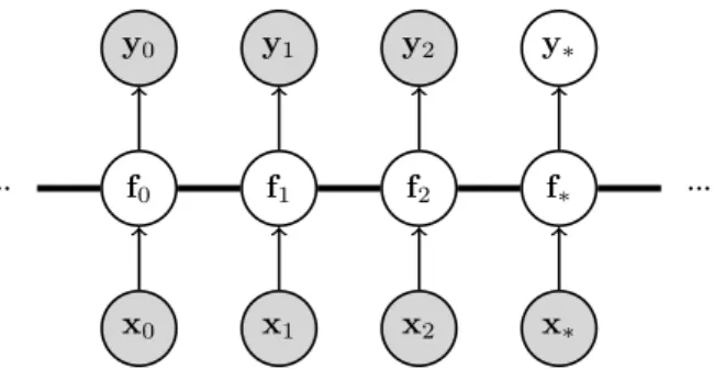
A possible way to represent Gaussian processes in a graphical model consists in drawing a thick solid bar between the jointly normally-distributed variables (Rasmussen and Williams, 2006). All the variables that touch the solid bar be-long to the same Gaussian process and are fully interconnected, i.e. in principle no conditional independence statements between those variables can be made until one examines the covariance function. There are an infinite amount of variables in the Gaussian process but we only draw a finite set. Periods of ellipsis can be drawn at the extremities of the solid bar to reinforce this idea.

Figure 2.3 depicts the model for Gaussian process regression with a dataset consisting of three inputs and three outputs and where predictions are to be made at a given test pointx∗.

x0 x1 x2 x∗

f0 f1 f2 f∗

y0 y1 y2 y∗

... ...

Figure 2.3: Graphical model of Gaussian process regression.

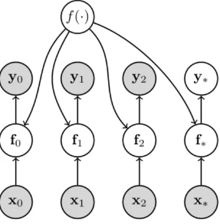
A way to interpret this notation consists in considering a functionf(·)that is distributed according to a GP. All variablesf are conditionally independent of each other given that function (Figure 2.4).

x0 x1 x2 x∗

f0 f1 f2 f∗

y0 y1 y2 y∗

Figure 2.4: Graphical model of Gaussian process regression explicitly representing the latent functionf(·).

It is important to note that models involving the thick bar shouldnotbe in-terpreted as a conventional undirected probabilistic graphical model. The thick bar notation shows in a simple manner which variables belong to the same GP. For general covariance functions, drawing Figure 2.3 with the semantics of con-ventional directed graphical models would result in a large number of edges. See Figure 2.5 for an example.

x0 x1 x2 x∗

f0 f1 f2 f∗

y0 y1 y2 y∗

Figure 2.5: Graphical model of Gaussian process regression using only directed edges.

2.3

A Z

OO OF

GP-B

ASED

D

YNAMICAL

S

YSTEM

M

ODELS

In this section we present a unified description of several models of dynamical systems based on Gaussian process that have appeared in the literature. In particular, we provide generative models to easily identify the assumptions made by each model and review the different inference/learning algorithms that have been tailored to each model.

The models based on Gaussian processes presented in this section are in fact generalisations of parametric models with similar structures. For instance, if the covariance functions in the GPs of the model shown in Section 2.3.5 are selected to be linear, the model becomes equivalent to the usual linear (para-metric) state-space model.

Furthermore, the equivalence theorem presented in Section 3.2.1 implies that several GP-based state-space models that have originally been presented as different in the literature are in fact equivalent. Those equivalences will be highlighted in the description of each model.

2.3.1

L

-G

T

S

M

Description: Many popular linear-Gaussian time series models can be in-terpreted as Gaussian processes with a particular covariance function and time as the index set of the GP. This includes linear auto-regressive models, lin-ear auto-regressive moving-average models, linlin-ear state-space models2_{, etc. A}

characteristic of these models is that all observationsy1:T arejointly Gaussian. Linear-Gaussian time series models have been studied in the classical time se-ries literature (Box et al., 1994), stochastic processes literature (Grimmett and Stirzaker, 2001) and also from a Gaussian process perspective (Turner, 2011; Roberts et al., 2012).

Inference and Learning: There is a rich literature about learning models of various flavours of linear auto-regressive models. Both maximum likelihood and Bayesian learning approaches have been described (Box et al., 1994; Ljung, 1999).

Inference in linear-Gaussian state-space models can be performed efficiently with the Kalman filter/smoother. Their use leads toO(T)exact inference rather than the naiveO(T3_{). Learning in linear-Gaussian state-space models has been}

tackled with approaches such as maximum likelihood (Shumway and Stoffer, 1982; Ljung, 1999), subspace methods (a type of spectral learning) (Overschee and Moor, 1996), and variational Bayes (Barber and Chiappa, 2006).

A different approach is to treat the problem as Gaussian process regres-sion with common covariance functions such as the squared exponential which specifies correlations that decay with time difference or periodic covariance functions that impose a period to the signal. See, for instance, (Roberts et al., 2012) for a recent overview of this approach and (Duvenaud et al., 2013) for an algorithm to perform search in the space of GP kernels. It is important to note, however, that GP regression from time to observations has an important drawback: it is not able to learn nonlinear dynamics. For example, consider a nonlinear aerobatic aeroplane. A model such as the one in this section can be useful to filter or interpolate data from a given test flight. However, it will not be able to learn a model of the aeroplane nonlinear dynamics suitable to create a flight simulator.

2_{Sometimes known as Kalman filters although this name can lead to confusion between the} model and the algorithm that is used to perform efficient exact inference on it.

2.3.2

N

A

-R

M

GP

Graphical model:

y0 y1 y2 y3 y4

f2 f3 f4

... ...

Second order model, i.e.Yt−1={yt−1,yt−2}. Generative model: f(Y)∼ GP mf(Y), kf(Y,Y0) , (2.15a) Yτy−1∼p(Yτy−1), (2.15b) ft=f(Yt−1), (2.15c) yt|ft∼p(yt|ft,θ), (2.15d) where Yt−1={yt−1, ...,yt−τy}. (2.15e)

Description: Auto-regressive models describe a time series by defining a mapping from past observations to the current observation. In the case of additive noise this is equivalent to

yt=f(yt−1, ...,yt−τy) +δt.

Conceptually, in other to generate data from this model, one would initially draw a function from Equation (2.15a) and draw the firstτy observations (Eq. (2.15b)). Then,the rest of the variables could be drawn sequentially. In practice, however, it is not generally possible to sample a whole function from the GP since it is an infinite dimensional object. Confer to section 3.1 for a discussion on how to draw samples in practice in a related model.

An important characteristic of this model is that there is no measurement noise such as that in a state-space model. Here, noise injected viaδthas an influence on thefuture trajectoryof the system.

Nonlinear auto-regressive models with external (exogenous) inputs are of-ten known as NARX models.

Inference and Learning: Learning in this model is performed using con-ventional GP regression techniques. Given a Gaussian process prior on the latent function, all flavours of Gaussian process regression can be applied to this model. In particular, exact inference is possible if we choose a conjugate likelihood, e.g.p(yt|ft,θ) =N(yt|ft,R).

Gregorcic and Lightbody (2002) and Kocijan et al. (2003) presented learn-ing of a GP-based NARX model via maximisation of the marginal likelihood. Girard et al. (2003) proposed a method to propagate the predictive uncertainty

in GP-based NARX models for multiple-step ahead forecasting. More recently, Gutjahr et al. (2012) have proposed the use of sparse Gaussian processes in order to reduce computational complexity and to scale to time series with mil-lions of data points.

2.3.3

S

-S

M

T

GP

Description: This model corresponds to a nonlinear state-space model where a Gaussian process prior has been placed over the state transition func-tionf(xt). This model can be seen as a generalisation of the parametric state-space model described by

xt+1|xt∼ N( ˜f(xt,θx),Q), (2.17a)

yt|xt∼p(yt|xt,θy). (2.17b) The Gaussian process prior overf(xt), equation (2.16a), can model systematic departures from the nonlinear parametric transition functionf˜(xt,θx), equa-tion (2.17a). In practice, one can encode inmf(xt)prior knowledge about the transition dynamics. For example, in the case of modelling a physical system, mf(xt)can be based on equations of the underlying physics. But those equa-tions need not perfectly describe the system. Dynamics not modelled inmf(xt) can be captured in the posterior overf(xt).

Following the theorem in Section 3.2.1, this model is equivalent to the mod-els in Sections 2.3.4 and 2.3.5. However, in general, converting the modmod-els in Sections 2.3.4 and 2.3.5 to a “transition-only GP-SSM” form requires an increase in the dimensionality of the state-space fromdim(xt)todim(xt) + dim(yt).

Inference and Learning: Frigola et al. (2013) derived a factorised formu-lation of the (non-Gaussian) prior over state trajectoriesp(x0:T)in the form of a product of Gaussians. This formulation made possible the use of a Parti-cle Markov Chain Monte Carlo (PMCMC) approach especially suited to non-Markovian models. In this approach, the joint smoothing posteriorp(x0:T|y0:T) is sampled directly without the need to knowf(x)which has been marginalised.

Note that this is markedly different to the conventional approach in parametric models where the smoothing distribution is obtained conditioned on a model of the dynamics. A related approach seeking a maximum (marginal) likelihood estimate of the hyper-parameters via Stochastic Approximation EM was pre-sented in (Frigola et al., 2014b). Finding point estimates of the hyper-parameters can be particularly useful when it is not obvious how to specify a prior over those parameters, e.g. for the inducing input locations in sparse GPs. Chap-ter 4 provides an expanded exposition of those learning methods based on PMCMC.

McHutchon and Rasmussen (2014) and McHutchon (2014) used a paramet-ricmodel for the state transition function inspired by the form of a GP regres-sion posterior akin to that presented in (Turner et al., 2010). They compared several inference and learning schemes based on analytic approximations and sampling. Learning was performed by finding maximum likelihood estimates of the parameters of the state transition function and the hyper-parameters.

Wu et al. (2014) used a state-space model with transition GP to model volatil-ities in a financial time-series setting. They presented an online inference and learning algorithm based on particle filtering.

2.3.4

S

-S

M

E

GP

Description: As opposed to the state-space model with transition GP, in this model the state transition has a parametric form whereas a GP prior is placed over the emission functiong(x).

Ifp(yt|gt,θy) =N(yt|gt,R)it is possible to analytically marginaliseg(x) to obtain a Gaussian likelihoodp(y0:T | x0:T)with a potentially non-diagonal covariance matrix.

Following the theorem in Section 3.2.1, this model is equivalent to the tran-sition GP model (Section 2.3.3). Moreover, if the parametric state trantran-sition in this model is linear-Gaussian, it can be considered a special case of the GP-LVM with GP on the latent variables (Section 2.3.7).

Inference and Learning:Ferris et al. (2007) introduced this model as a GP-LVM with a Markovian parametric density on the latent variables. The model was learnt by finding maximum a posteriori (MAP) estimates of the states.

2.3.5

S

-S

M

T

E

GP

Description: This model results from a combination of the models in Sec-tions 2.3.3 and 2.3.4. However, perhaps surprisingly, the theorem presented in Section 3.2.1 shows that this model is equivalent to the transition GP model (Section 2.3.3). Therefore, inference methods designed for the transition GP model can be used here after a straightforward redefinition of the state vari-able.

Placing GP priors over both the state transition and the emission functions opens the door to non-identifiability issues. Those can be mitigated to some extent by a judicious choice of the parametrisation of the mean and covariance functions (or by placing priors over those hyper-parameters). However, if the latent states do not correspond to any interpretable quantity and the only goal is prediction, the non-identifiability is a problem of lesser importance.

Wang et al. (2006, 2008) presented this model in terms of the weight-space view of Gaussian processes (Rasmussen and Williams, 2006) where an infi-nite number of weights are marginalised. The expression for p(y0:T|x0:T)is straightforward since it corresponds to the Gaussian distribution describing the marginal likelihood of the GP regression model. However, p(x0:T)is, in their own words, “more subtle” since a regression approach would lead to “the nonsensical expressionp(x2, ...,xN|x1, ...,xN−1)”. After marginalisation,

Wang et al. obtain an analytic expression for the non-Gaussianp(x0:T). In Chapter 3 of this dissertation, we provide an alternative derivation ofp(x0:T) which leads to a number of insights on the model that we use to derive new learning algorithms.

Inference and Learning: Wang et al. (2006) obtained a MAP estimate of the latent state trajectory. Later, in (Wang et al., 2008), they report that MAP learning is prone to overfitting for high-dimensional states and suggest two solutions: 1) a non-probabilistic regularisation of the latent variables, and 2) maximising the marginal likelihood with Monte Carlo Expectation Maximi-sation where the joint smoothing distribution is sampled using Hamiltonian Monte Carlo.

Ko and Fox (2011) use weak labels of the state to obtain a MAP estimate of the state trajectory and hyper-parameters. The weak labels of the state are actually direct observations of the state contaminated with Gaussian noise. Somehow, this is not the spirit of the model which should “discover” what the state representation is given any sort of observations. In other words, weak labels are nothing else than a particular type of observation that gives a glimpse into what the state actually is. (Note that Ko and Fox (2011) has a crucial technical problem in its Equation 14 which leads to the expression

p(x2, ...,xN−1,xN|x1,x2, ...,xN−1)that Wang et al. (2006) had successfully sidestepped.

In Chapter 3 of this thesis we provide a novel formulation of the model that sheds light on this issue.)

Turner et al. (2010) presented an approach to learn a model based on the state-space model with transition an emission GPs. They propose a parametric model for the latent functionsf(x)andg(x)that takes the form of a posterior from Gaussian process regression whose input and output “datasets” are pa-rameters to be tuned. A point estimate of the papa-rameters forf(x)and g(x)

is learnt via maximum likelihood with Expectation Maximisation while treat-ing the state trajectory as latent variables. Several approaches for filtertreat-ing and smoothing in this kind of models have been developed (Deisenroth et al., 2012; Deisenroth and Mohamed, 2012; McHutchon, 2014). A related model was pre-sented in (Ghahramani and Roweis, 1999) where the nonlinear latent functions take the shape of Gaussian radial basis functions (RBFs) and learning is per-formed with the EM algorithm using an Extended Kalman Smoother for the E-step.

2.3.6

N

-M

-S

M

T

GP

Second order model, i.e.Xt−1={xt−1,xt−2}. Generative model: f(X)∼ GP mf(X), kf(X,X0) , (2.20a) Xτx−1∼p(Xτx−1), (2.20b) ft=f(Xt−1), (2.20c) xt|ft∼ N(ft,Q), (2.20d) yt|xt∼p(yt|xt,θy), (2.20e) where Xt−1={xt−1, ...,xt−τx}. (2.20f)

Description: This model is equivalent to a Markovian SSM (Section 2.3.3) with a new state defined aszt = {xt, ...,xt−τx+1}. The reason for explicitly

including this model in the present review is that it can also be seen as a gener-alisation of a nonlinear auto-regressive model (Section 2.3.2) with observation noise.

Inference and Learning:As opposed to auto-regressive models, the present model explicitly takes measurement noise into account. The observations y

can be considered noisy versions of some latent, uncorrupted, variablesx. Ob-servation noise in Equation (2.20e) does not affect the future trajectory of the system. Rigorous inference and learning in this model is as computationally demanding as for the equivalent Markovian SSM (Section 2.3.3). However, in (Frigola and Rasmussen, 2013) we proposed a fast approximate method that simultaneously filtersy to approximatex and learns an auto-regressive model on the approximate x. Any parameter from the preprocessing stage (e.g. the cut-off frequency of a low pass filter) is optimised jointly with the hyper-parameters of the model. See Chapter 6 for more details.

Another approach is to use GP regression with uncertain inputs (McHutchon and Rasmussen, 2011; Damianou and Lawrence, 2015) to learn the auto-regressive function. Note that this is also an approximation since it does not take into account that some inputs to the regression problem are also outputs, e.g. x2

2.3.7

GP-LVM

GP

L

V

Description: This model can be interpreted as a particular case of a Gaus-sian process latent variable model (GP-LVM, Lawrence (2005)) where the spher-ical prior over latent variables has been substituted by a second Gaussian pro-cess. This Gaussian process provides temporal correlations between the la-tent variables which become a low-dimensional representation of the high-dimensional observationsy.

There is no explicit modelling of a nonlinear transition between successive latent statesxt. However, the use of a kernelkx(t, t0) such as the Ornstein-Uhlenbeck covariance function would result in dynamics on the latent states equivalent to those of a linear-Gaussian state-space model. Unfortunately, non-linear state transitions, which are one of the strengths of GP-based state-space models, can not be modelled.

Inference and Learning: Lawrence and Moore (2007) introduced this model and sought a maximum a posteriori (MAP) solution with respect to the latent statesxt. More recently, Damianou et al. (2011) proposed a variational learning algorithm that builds on the techniques developed for the Variational Bayesian GP-LVM of Titsias and Lawrence (2010). This approach does not suffer from the overfitting problems of the MAP solution and automatically determines the dimensionality of the latent space whenkg(x,x0)is chosen to be an automatic relevance determination (ARD) kernel. An extension of this work to models with deeper hierarchies has resulted in deep Gaussian processes (Damianou and Lawrence, 2013).

Latent force models (Alvarez et al., 2009, 2013) can also be interpreted as a particular case of GP-LVM with a GP on the latent variables. The variables

xin the top layer are the latent forces whereas theglayer encodes the linear-Gaussian stochastic differential equation of the latent force model.

2.4

W

HY

G

AUSSIAN

P

ROCESS

S

TATE

-S

PACE

M

OD

-ELS

?

Gaussian Process State-Space Models are particularly appealing because they enjoy the generality of nonlinear state-space models together with the flexi-ble prior over the transition function provided by the Gaussian process. As opposed to auto-regressive models, the presence of a latent state allows for a succinct representation of the dynamics in the form of a Markov chain. The state needs to contain only the information about the system that is essential to determine its future trajectory. As a consequence, discovering a state represen-tation for a system provides useful insights about its nature since it decouples the observations that happen to be available from the dynamics.

A related advantage of state-space models over auto-regressive ones is that observation noise can be explicitly taken into account. To train an auto-regressive model, a time series is broken down into a set of input/output pairs and the function mapping inputs to outputs is learnt with regression techniques. One could use noise-in-the-inputs regression (also known as errors-in-variables) to deal with observation noise. However, this would fail to exploit the fact that the particular noise realisation affecting the observationytis the same when using yt as an input or as an output. When learning a state-space model, the time series is not broken down into input/output pairs and inference and learning are performed in a way that coherently takes into account observation noise. This will be clearer in the learning algorithms of the following chapters.

Gaussian Process State-Space

Models – Description

”Trying to understand a hidden Markov model from its observed time se-ries is like trying to figure out the workings of a noisy machine from look-ing at the shadows its movlook-ing parts cast on a wall, with the proviso that the shadows are cast by a randomly-flickering candle.”

Shalizi (2008)

This chapter presents a novel formalisation of Gaussian Process State-Space Models (GP-SSMs). In particular, we go beyond describing the joint probabil-ity of the model and provide a practical approach to generate samples from its prior. The insights provided by the new description of GP-SSMs will be ex-ploited in the next chapters to derive learning and inference methods adapted to the characteristics of the model. In addition, we present an equivalence re-sult stating that GP-SSMs with GP priors on the transition and emission func-tions can be reformulated into GP-SSMs with a GP only on the state transition function.

3.1

GP-SSM

WITH

S

TATE

T

RANSITION

GP

As presented in Section 2.3, there exist many flavours of GP-SSMs. For clarity, in this section we shall restrict ourselves to a GP-SSM which has a Gaussian process prior on the transition function but a parametric density to describe the likelihood (i.e. the model introduced in Section 2.3.3). This particular model contains the main feature that has made GP-SSMs hard to describe rigorously: the states are simultaneously inputs and outputs of the state transition func-tion. In other words, we want to learn a function whose inputs and outputs are not only latent but also connected in a chain-like manner.

Given an observed time series{y1, ...,yT}, we construct a stochastic model 25

that attempts to explain it by defining a chain of latent states{x0, ...,xT}

xt|xt−1∼ N(xt|f(xt−1),Q), (3.1a) yt|xt∼p(yt|xt,θy), (3.1b) wheref(·)in an unknown nonlinear state transition function andQandθyare parameters of the state transition density and likelihood respectively. A com-mon way to learn the unknown state transition function is to define a para-metric form for it and proceed to learn its parameters. Common choices for parametric state transition functions are linear functions (Shumway and Stof-fer, 1982), radial basis functions (RBFs) (Ghahramani and Roweis, 1999) and other types of neural networks.

GP-SSMs do not restrict the state transition function to a particular parame-terised class of functions. Instead, they place a Gaussian process prior over the infinite-dimensional space of functions. This prior can encode assumptions such as continuity or smoothness. In fact, with an appropriate choice of the covariance function, the GP prior puts probability mass over all continuous functions (Micchelli et al., 2006). In other words, as opposed to parameterised functions, GPs do not restrict a priori the class of continuous functions that can be learnt provided that one uses covariance functions that are universal kernels (Micchelli et al., 2006). The squared exponential is an example of such a kernel. The generative model for a GP-SSM with a GP prior over the state transition function and an arbitrary parametric likelihood is

f(x)∼ GP m(x), k(x,x0) , (3.2a) x0∼p(x0), (3.2b) ft=f(xt−1), (3.2c) xt|ft∼ N(xt|ft,Q), (3.2d) yt|xt∼p(yt|xt,θy). (3.2e) In order to get an intuitive understanding of this model, it can be useful to devise a method to generate synthetic data from it. An idealised approach to generate data from a GP-SSM could consist in first sampling a state transition function (i.e. an infinite-dimensional object) from the GP. This only needs to happen once. Then the full sequence of states can be generated by first sam-pling the initial statex0and then sequentially sampling the rest of the chain {f1,x1, ...,fT,xT}. Each observationytcan be sampled conditioned on its cor-responding statext.

However, this idealised sampling procedure can not be implemented in practice. The reason for this is that it is not possible to sample an infinite-dimensional function and store it in memory. Instead, we will go back to the definition of a Gaussian process and define a practical sampling procedure for the GP-SSM.

number of which have a joint Gaussian distribution (Rasmussen and Williams, 2006). However, in a GP-SSM, there is additional structure linking the vari-ables. A sequential sampling procedure provides insight into what this struc-ture is. To sampleft, instead of conditioning on an infinite-dimensional func-tion, we condition only on the transitions {xi−1,fi}ti−=11seen up to that point.

For a zero-mean GP x0∼p(x0), (3.3a) f1|x0∼ N(f1|0, k(x0,x0)), (3.3b) x1|f1∼ N(x1|f1,Q), (3.3c) f2|f1,x0:1∼ N(f2|k(x1,x0)k(x0,x0)−1f1, k(x1,x1)−k(x1,x0)k(x0,x0)−1k(x0,x1)), (3.3d) x2|f2∼ N(x2|f2,Q), (3.3e) f3|f1:2,x0:2∼ N(f3|[k(x2,x0) k(x2,x1)] " k(x0,x0) k(x0,x1) k(x1,x0) k(x1,x1) #−1" f1 f2 # , k(x2,x2)−[k(x2,x0) k(x2,x1)] " k(x0,x0) k(x0,x1) k(x1,x0) k(x1,x1) #−1" k(x0,x2) k(x1,x2) # ), (3.3f) .. .

Since this notation is very cumbersome, we will use the shorthand notation for kernel matrices

Ki:j,k:l,     k(xi,xk) . . . k(xi,xl) .. . ... k(xj,xk) . . . k(xj,xl)     , (3.4)

and Ki:j , Ki:j,i:j. Note that the covariance functionk(·,·)returns a matrix of the same size as the state in an analogous manner to multi-output Gaussian processes (Rasmussen and Williams, 2006). With this notation, equations (3.3) become x0∼p(x0), (3.5a) f1|x0∼ N(f1|0,K0), (3.5b) x1|f1∼ N(x1|f1,Q), (3.5c) f2|f1,x0:1∼ N(f2|K1,0K−01f1, K1,1−K1,0K−01K0,1), (3.5d) x2|f2∼ N(x2|f2,Q), (3.5e) f3|f1:2,x0:2∼ N(f3|K2,0:1K−0:11f1:2, K2,2−K2,0:1K−0:11K0:1,2), (3.5f) .. .

0 time states 0 time 0 time 0 time

Figure 3.1: State trajectories from four 2-state nonlinear dynamical systems sampled from a GP-SSM prior with identical hyperparameters. The same prior generates systems with quali-tatively different behaviours, e.g. the leftmost panel shows behaviour similar to that of a non-oscillatory linear system whereas the rightmost panel appears to have arisen from a limit cycle in a nonlinear system.

For a general time step, the key density is

p(ft|f1:t−1,x0:t−1) =N(ft|Kt−1,0:t−2K0:−1t−2f1:t−1,

Kt−1,t−1−Kt−1,0:t−2K−0:1t−2K0:t−2,t−1), (3.6)

which is analogous to the predictive density in GP regression. In particular, it corresponds to the prediction at a single test pointxt−1using inputsx0:t−2and

noiselessoutputsf1:t−1.

The joint distribution over latent and observed variables can be expressed as p(y1:T,x0:T,f1:T) =p(x0) T Y t=1 p(yt|xt)p(xt|ft)p(ft|f1:t−1,x0:t−1). (3.7)

The behaviour of GP-SSMs is demonstrated in Figure 3.1 which shows four independent state trajectories sampled from a GP-SSM. Equations (3.5) pro-vided the sequential procedure used for sampling. The richness of the nonlin-ear dynamics allowed by a squared exponential kernel allow for very different qualitative behaviour.

3.1.1

A

I

R

At this point, it is useful to note that T

Y

t=1

p(ft|f1:t−1,x0:t−1) =N f1:T |0,K0:T−1. (3.8)

Equation (3.8) provides a “telescopic” expression where eachftdepends on the previousf1:t−1andx0:t−1. The conditioning onxonly up to timet−1is critical.

If we were to condition on the full state trajectoryx0:T, the distribution over

f1:T would be markedly different. In particular, we would be facing a problem akin to GP regression where we would be looking at the posterior distribution over the latent function values conditioned on inputsx0:T−1andnoisyoutputs

x1:T

p(f1:T |x0:T) =N f1:T |K0:T−1Ke−_0:1_T−1x1:T,

K0:T−1−K0:T−1Ke−_0:1_T−1K>_0:T−1

, (3.9)

withKe0:T−1,K0:T−1+IT⊗Q. As one could expect, this expression reduces tof1:T =x1:T ifQ=0.

We can summarise the previous argument by stating that T Y t=1 p(ft|f1:t−1,x0:t−1) =N f1:T |0,K0:T−1 6 =p(f1:T |x0:T). (3.10) For completeness, we provide the expressions for an arbitrary mean func-tion where we usem0:t,[m(x0)>, ..., m(xt)>]>:

T Y t=1 p(ft|f1:t−1,x0:t−1) =N f1:T |m0:T−1,K0:T−1 , (3.11) and p(f1:T |x0:T) =N f1:T |m0:T−1+K0:T−1Ke− 1 0:T−1(x1:T−m0:T−1), K0:T−1−K0:T−1Ke− 1 0:T−1K > 0:T−1 . (3.12)

3.1.2

M

f

By marginalising out the variablesf1:T we will obtain a prior distribution over state trajectories that will be particularly useful for learning GP-SSMs with sample-based approaches (Chapter 4). The density over latent variables in a GP-SSM is p(x0:T,f1:T) =p(x0) T Y t=1 p(xt|ft)p(ft|f1:t−1,x0:t−1) (3.13a) =p(x0)N(x1:T |f1:T,IT ⊗Q)N(f1:T |m0:T−1,K0:T−1). (3.13b)

Marginalising with respect to f1:T we obtain the prior distribution over the latent state trajectory

p(x0:T) = Z p(x0:T,f1:T) df1:T (3.14a) =p(x0) Z N(x1:T |f1:T,IT ⊗Q)N(f1:T |m0:T−1,K0:T−1) df1:T (3.14b) =p(x0)|(2π)nxTKe0:T−1|− 1 2exp(−1 2(x1:T −m0:T−1) > e K−_0:1_T−1(x1:T −m0:T−1)), (3.14c) which is the density provided in (Wang et al., 2006) albeit in a slightly different form.

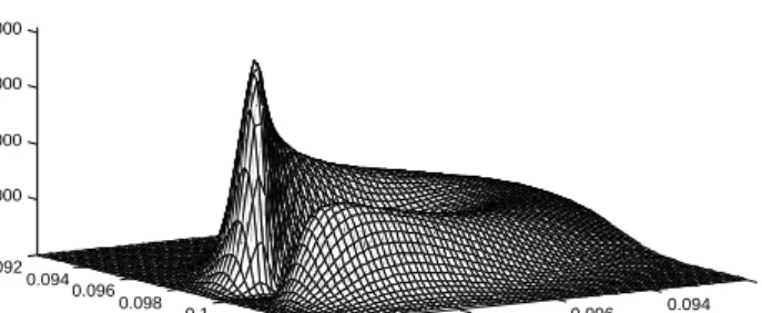
0.092 0.094 0.096 0.098 0.1 0.092 0.094 0.096 0.098 0.1 0.102 0.104 2000 4000 6000 8000 x₁ x 2 p(x 1 ,x2 |x0 ,x3 )

Figure 3.2: Density functionp(x1:2|x0= 0.1, x3= 0.095)for a one-state GP-SSM.

To solve the integral in equation 3.14b we have used a standard result from integrating a product of Gaussians. However, the resulting distribution isnot Gaussian. The fact thatK0:T−1 already depends onx0:T−1 results in

equa-tion (3.14c) not being Gaussian inx0:T. This is clear in Figure 3.2 which shows how the conditional distributions ofp(x0:3)are far from Gaussian.

Although the prior distribution over state trajectoriesp(x0:T)is not Gaus-sian, it can be expressed as a product of Gaussians

p(x0:T) =p(x0) T Y t=1 p(xt|x0:t−1) (3.15a) =p(x0) T Y t=1 N xt|µt(x0:t−1),Σt(x0:t−1) , (3.15b) with µ_t(x0:t−1) =mt−1+Kt−1,0:t−2Ke−_0:1_t−2(x1:t−1−m0:t−2), (3.15c) Σt(x0:t−1) =Ket−1−Kt−1,0:t−2Ke−_0:1_t−2K>_{t−1,0:t−2} (3.15d)

fort ≥ 2 and µ₁(x0) = m0, Σ1(x0) = Ke0. Equation (3.15b) follows from

the fact that, once conditioned onx0:t−1, the distribution overxtcorresponds to the predictive density of GP regression at a single test point xt−1

condi-tioned on inputsx0:t−2 andnoisy outputsx1:t−1. Note that naive evaluation

of Equation (3.15) has complexityO(T4_{)whereas Equation (3.14) can be}

eval-uated straightforwardly inO(T3_).

3.1.3

M

f

(

x

)

So far in this chapter, we have provided a constructive method to obtain the joint probability density of a GP-SSM. This approach sidestepped having to deal with infinite-dimensional objects. Here, following (Turner et al., 2015), we re-derive the density over the latent variables of a GP-SSM by starting from a joint distribution containing a Gaussian process and marginalising it to obtain a joint distribution over a finite number of variables. The goal of the presenta-tion below is to provide an intuipresenta-tion for the marginalisapresenta-tion of the latent func-tionf(·). Strictly speaking, however, conventional integration over an infinite dimensional object such asf(·)is not possible and the derivation below should

be considered just a sketch. We refer the reader to (Matthews et al., 2015) for a much more technical exposition of integration of infinite dimensional objects in the context of sparse Gaussian processes.

We start with a joint distribution of the state trajectory and the random functionf(·) p(x0:T, f(·)) =p(f(·))p(x0) T Y t=1 p(xt|xt−1, f(·),Q), (3.16)

and introduce new variablesft=f(xt−1)which, in probabilistic terms can be

defined as a Dirac deltap(ft|f(·),xt−1) =δ(ft−f(xt−1)). p(x0:T,f1:T, f(·)) =p(f(·))p(x0)

T

Y

t=1

p(xt|ft,Q)p(ft|f(·),xt−1), (3.17)

By integrating the latent function at every point other thanx0:T−1we obtain p(x0:T,f1:T) = Z p(x0:T,f1:T, f(·)) df\x0:T−1 (3.18a) =p(x0) T Y t=1 N(xt|ft,Q) ! Z p(f(·)) T Y t=1 δ(ft−f(xt−1)) df\x0:T−1 (3.18b) =p(x0)N(x1:T |f1:T,IT ⊗Q)N(f1:T |m0:T−1,K0:T−1), (3.18c)

which recovers the joint density from equation (3.13b)

3.2

GP-SSM

WITH

T

RANSITION AND

E

MISSION

GP

S

GP-SSMs containing a nonlinear emission function with a GP prior have also been studied in the literature (see Section 2.3.5). In such a model, the nonlinear functiong(xt)in the state-space model

xt|xt−1∼ N(xt|f(xt−1),Q), (3.19a) yt|xt∼ N(yt|g(xt),R), (3.19b) also has a GP prior which results in a generative model described by

f(x)∼ GP mf(x), kf(x,x0), (3.20a) g(x)∼ GP mg(x), kg(x,x0), (3.20b) x0∼p(x0), (3.20c) ft=f(xt−1), (3.20d) xt|ft∼ N(xt|ft,Q), (3.20e) gt=g(xt), (3.20f) yt|gt∼ N(yt|gt,R). (3.20g)

This variant of GP-SSM is a straightforward extension to the one with a parametric observation model. The distribution over latent states and tran-sition function values is the same. However, an observation at timet isnot conditionally independent of the rest of the observations givenxt. The joint probability distribution of this model is

p(y1:T,g1:T,x0:T,f1:T) =p(x0:T,f1:T)p(g1:T|x1:T) T Y t=1 p(yt|gt) (3.21a) =p(x0:T,f1:T)N(g1:T |m (g) 1:T,K (g) 1:T) T Y t=1 N(yt|gt,R). (3.21b) Wherep(x0:T,f1:T)is the same as in Equation (3.7) andm(g)andK(g)denote the mean function vector and kernel matrix using the mean and covariance functions in Equation (3.20b).

3.2.1

E

GP-SSM

In the following, we present an equivalence result between the two GP-SSM variants introduced in this chapter. We show how the model with nonlineari-ties for both the transition and emission functions (Sec. 2.3.5 and 3.2) is equiv-alent to a model with a redefined state-space but which only has a nonlinear function in the state transition (Sec. 2.3.3 and 3.1).

We consider state-space models with independent and identically distributed additive noise

xt+1=f(xt) +vt, (3.22a)

yt=g(xt) +et. (3.22b)

In GP-SSMs, Gaussian process priors are placed overf andg in order to perform inference on those functions.

THEOREM: The model in (3.22) is a particular case of the following model

zt+1=h(zt) +wt, (3.23a)

yt=γγγt+et, (3.23b)

wherezt,(ξξξt, γγγt)is theaugmented state. PROOF: Consider the case where

Then, the model in (3.23) can be written as

ξξξt+1=f(ξξξt) +νννt, (3.25a)

γγγt+1=g(ξξξt), (3.25b)

yt=γγγt+et. (3.25c)

If we now takeξξξt=xt+1andνννt=vt+1and substitute them in (3.25) we obtain

xt+1=f(xt) +vt, (3.26a)

yt=g(xt) +et. (3.26b)

COROLLARY: A learning procedure that is able to learn an unknown state tran-sition function can also be used to simultaneously learnbothf(xt)andg(xt).

3.3

S

PARSE

GP-SSM

S

Gaussian processes are very useful priors over functions that, in comparison with parametric models, place very few assumptions on the shapes of the un-known functions. However, this richness comes at a price: computational re-quirements for training and prediction scale unfavourably with the size of the training set. To alleviate this problem, methods relying onsparse Gaussian pro-cesseshave been developed that retain many of the advantages of vanilla Gaus-sian processes while reducing the computational cost (Qui ˜nonero-Candela and Rasmussen, 2005; Titsias, 2009; Hensman et al., 2013, 2015).

Sparse Gaussian processes often rely on a number of inducing points. Those inducingpoints, denoted byui, are values of the unknown function at arbitrary locations named inducinginputs

ui=f(zi). (3.27)

For conciseness of notation, we define the set with all inducing points u _, {ui}Mi=1 and the set of their respective inducing inputs z , {zi}Mi=1. If we

place a Gaussian process prior over a functionf, the inducing points are jointly Gaussian with values of the latent function at any other location

p(f,u) =N " f u # " mx mz # , " Kx Kx,z Kz,x Kz #! . (3.28)

This method of explicitly representing the values of the function at an ad-ditional finite number of input locationszis sometimes called augmentation. However, one could argue that the model has not been augmented since the in-ducing points were “already there”; we are simply assigning a variable name to the value of the function at input locationsz.

making additional assumptions on the relationships between function values at the training, test and inducing inputs (Qui ˜nonero-Candela and Rasmussen, 2005). More recently, a variational approach to sparse GPs (Titsias, 2009) has resulted in sparse GP methods for a number of models (Titsias and Lawrence, 2010; Damianou et al., 2011; Hensman et al., 2013, 2015).

In Chapter 5 we will develop a variational inference approach for GP-SSMs. It is then useful at this point to provide an explicit description of a GP-SSM with inducing points. The latent variables of such a GP-SSM have the following joint density p(x0:T,f1:T,u|z) =p(u|z)p(x0) T Y t=1 p(xt|ft)p(ft|f1:t−1,x0:t−1,u,z), (3.29)

wherep(u|z) =N(mz,Kz). To lighten the notation, from now on we will omit

the explicit conditioning on inducing inputsz. The product of latent function conditionals can be succinctly represented by the following Gaussian

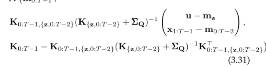
T Y t=1 p(ft|f1:t−1,x0:t−1,u) =N f1:T |m0:T−1+K0:T−1,zK−z1(u−mz), K0:T−1−K0:T−1,zK−z1K>0:T−1,z , (3.30) which is equivalent to the predictive density of GP regression with inputsz, noiselessoutputsuand test inputsx0:T−1. We emphasise again that this

tele-scopic product of conditionals isnotthe same as p(f1:T|x0:T−1,u) =N m0:T−1+ K0:T−1,{z,0:T−2}(K{z,0:T−2}+ ΣΣΣQ)−1 u−mz x1:T−1−m0:T−2 ! , K0:T−1−K0:T−1,{z,0:T−2}(K{z,0:T−2}+ ΣΣΣQ)−1K0:>T−1,{z,0:T−2} (3.31) whereΣΣΣQ = blockdiag(0,I⊗Q) takes into account thatuare equivalent to

noiseless observations whereas neighbouring states are affected by process noise with covarianceQ.

In Section 5.7.1 we will highlight a number of parallelisms between sparse GP-SSMs and Recurrent Neural Networks: a class of neural networks that is currently receiving attention due to its ability to learn insightful representa-tions of sequences (Sutskever, 2013; LeCun et al., 2015).

3.4

S

UMMARY OF

GP-SSM D

ENSITIES

p(y1:T,x0:T,f1:T) Eq. (3.7) QT t=1p(ft|f1:t−1,x0:t−1) Eq. (3.11) p(f1:T|x0:T) Eq. (3.12) p(x0:T,f1:T) Eq. (3.13b) p(x0:T, f(·)) Eq. (3.16) p(x0:T) Eqs. (3.14) & (3.15) p(x0:T,f1:T,u|z) Eqs. (3.29) QT t=1p(ft|f1:t−1,x0:t−1,u) Eq. (3.30) p(f1:T|x0:T−1,u) Eq. (3.31)