An Efficient Technique for Clustering Data with Mixed Attribute Types

(1)

An Efficient Technique for Clustering Data with Mixed Attribute Types

Rahmah Brnawy

A Thesis

in

The Department

of

Computer Science and Software Engineering

Presented in Partial Fulfillment of the Requirements

for the Degree of Master of Computer Science

Concordia University

Montreal, Quebec, Canada

June 2015

(2)

CONCORDIA UNIVERSITY

School of Graduate Studies

This is to certify that the thesis prepared

By: Rahmah Brnawy

Entitled: An Efficient Technique for Clustering Data with Mixed Attribute Types

and submitted in partial fulfillment of the requirements for the degree of

Master of Computer Science

complies with the regulations of the University and meets the accepted standards with respect to originality and quality.

Signed by the final examining committee:

______________________________________ Chair Dr. Peter Rigby ______________________________________ Examiner Dr. Sudhir Mudur _____________________________________ Examiner Dr. Gösta Grahne ______________________________________ Supervisor Dr. Nematollaah Shiri

Approved by ________________________________________________ Chair of Department or Graduate Program Director

________________________________________________ Dean of Faculty Date ________________________________________________

(3)

iii

ABSTRACT

An Efficient Technique for Clustering Data with Mixed Attribute Types

Rahmah Brnawy

Clustering is a technique used to extract useful information and discover patterns from data. Existing clustering techniques have often focused on datasets with attributes that are either numeric or categorical but not both. The problem of clustering mixed numeric and categorical datasets has received increased attention more recently and a number of solutions have been proposed. In this research, we study these solutions and propose two clustering algorithms. The first algorithm that we present is called Cluc+, which extends and improves Cluc, an existing algorithm proposed for clustering pure categorical data. Using Cluc+, we then develop a new algorithm, called k-mixed for clustering data with mixed numeric and categorical attribute types. We conduct numerous experiments to evaluate the performance of our proposed algorithms using real-life benchmark datasets. Our results indicate increased efficiency and accuracy of the proposed solution techniques.

(4)

iv

ACKNOWLEDGMENTS

I am grateful to the Almighty God for helping me at all times including through the period of my study at Concordia University. I so much appreciate my supervisor, Dr. Nematollaah Shiri, for his patience and guidance. I cannot forget his encouragements through the learning curve of my research.

I would also like to extend my sincere gratitude to the Saudi Bureau and my alma mater –Tabiah University– for their financial support.

To my wonderful family: my Dad, Mom and siblings, I say thank you so much for all your love and care. Also, special thanks to my lovely sister, Ebtesam Barnawi, and to my best friend, Mr. Taiwo Adetiloye, who is currently pursuing his PhD study at CIISE, who made my stay at Concordia worthwhile.

(5)

v

Introduction

Chapter 1.

1.1. Cluster Analysis

A huge amount of data is produced and collected every day in different applications. Different mining techniques have been developed and deployed to extract useful information and discover patterns in the data using statistical techniques to obtain, e.g., mean, standard deviation, etc. However, such data often includes other hidden patterns and useful information that are far more valuable to find. This information and knowledge can assist in different application domains such as decisions making, medical diagnosis, business management, etc. Data analysis and mining tools are designed to discover such interesting knowledge and patterns from enormous amount of data.

Clustering is an important data-mining technique, which falls in the category of unsupervised learning techniques, as it does not use prior knowledge about the data and its structure [1]. The goal of clustering is to divide the input set of data/objects into homogenous groups (called clusters), such that objects within the same cluster are “similar” to each other and those placed in different clusters are “dissimilar” [1].

In this research, clustering structured data is considered, that is, every data item/object is described by a fixed set of attributes as in relational data. The types of data could be numeric or categorical, i.e., enumerated type. While clustering of numeric data enjoys a number of popular similarity measures such as Euclidean distance, clustering categorical data is often a challenge since there is no inherent distance measure between categorical values [2]. We refer to datasets described by attributes of the same type as pure datasets. The attributes of a pure dataset are either all of numeric type or they are all categorical. The class of pure datasets are then classified to pure numeric or pure categorical. Some datasets have a mix of numeric and categorical attributes.

(12)

2

There are numerous solutions proposed for clustering pure numeric data, such as k-mean [3], DBSCAN [4], CHAMELEON [5], and pure categorical data such as CURE [6], ROCK [7], CLUC [8]. Clustering data with mixed data types has received increased attention more recently.

Researchers have been looking for “suitable” ways to determine the “weights” of different attribute types to avoid biased results. Another problem that affects the performance of clustering data with mixed attribute types is that they often treat nominal and binary attributes equally. The previously proposed solutions paid less attention to the fact that binary attributes could be symmetric or asymmetric [2], and hence should not be given the same weights in the clustering process. This implies that a proper assignment of weights is crucial for a desired clustering algorithm to capture the different characteristics of the data.

Similarity measures are important for the performance of clustering pure or mixed data. Consider Figure 1 that was generated by Weka [9] which shows data distribution of a real-life dataset. As can be seen, the dataset contains 9 categorical attributes, of which C, D, E, F, and M are nominal with different distinct values, and A, H, I, and K are binary with two possible values. The distinct values of each attribute are represented by solid rectangles associated with a number on the top, which reflects the frequencies of the values in that attribute. For example, attribute “A” has two different values, therefore there are two sold rectangles. The frequency of one of its value is 488 and the other one is 222. The clustering of this dataset is influenced by the binary attributes, since one of the two values appears most frequently but carries less weight compared to the other value and other nominal values [2]. Since the similarity measures used in clustering categorical data are usually based on the co-occurrences and frequencies of the values, the high frequency of some values may lead to bias in the clustering result and poor quality in general. This suggests that, to improve the clustering quality, we need to reduce the influence of attributes with highly frequent values.

(13)

3

(14)

4

Clustering is a subjective task, in which applying different algorithms on the same dataset may produce several different and meaningful clustering results. For example, Figure 2 presents some tuples in a mixed dataset, called flag. The dataset includes information about 194 different countries and their flags. Different clustering solutions can be obtained from this dataset based on different points of views (attributes). Different algorithms may group these countries into different meaningful clusters. For instance, an algorithm may identify a religious icon or symbols on the flag of the country and classify them. It is also possible to cluster these countries into not so useful groups based on the number of lines in the flags or presence of certain color in the flags.

.

(15)

5

As mentioned above, not every cluster is meaningful and useful. Poor clustering results are usually obtained because the clustering process is influenced by wrong or useless parameters. For example, Figure 3(a) shows nine objects, which look quite similar. Grouping these objects into one cluster seem to make more sense. However, if the clustering algorithm requires the user to provide the number of clusters as an input parameter, this may result in a poor cluster, as shown in Figure 3(b). Thus, the quality of clustering depends on the underlying similarity measure used in the clustering process and/or on the user-predefined parameters provided. Therefore, it is crucial (1) to find a good similarity/dissimilarity function, and (2) to identify influential and meaningful input parameters.

Figure 3: Example of (a) good clustering (b) not so useful clustering

1.2. Thesis Contributions

The contributions of this thesis are as follows:

1. Developing k-mixed, a technique for clustering mixed datasets. This technique modifies and uses an existing clustering algorithm, called CLUC, that works on categorical datasets.

2. Performing extensive experiments on different datasets to evaluate the performance of k-mixed.

3. Implementing the k-mean algorithm for mixed attribute types and comparing its performance with k-mixed. Results are also compared with those obtained using well-known algorithms

4. Evaluating the performance of the developed technique in various aspects, including detecting and handling noise, scalability, and sensitivity to the order of the data.

(16)

6

1.3. Thesis Outline

The rest of this thesis report is organized as follows. Chapter 2 presents the background concepts and techniques in cluster analysis. Chapter 3 is a review of the related work. In Chapter 4, we review the CLUC algorithm and discuss ways to improve its performance in terms of quality. Using the revised CLUC, Chapter 5 presents a design and implementation of k-mixed, a new algorithm proposed in this thesis for clustering mixed datasets. In Chapter 6, we report the results of our experiments for performance evaluation of k-mixed using real-life benchmark datasets. Chapter 7 includes concluding remarks and outlines the future work.

(17)

7

Background, Definitions, and Concepts

Chapter 2.

2.1. Objects and Attributes

A dataset D is a collection of objects which consists of columns and rows. In clustering context, rows are the objects (also called tuples, records, observations, or data points) to be clustered into groups, and the columns are the attributes (also called domains, variables, or features). Each object in D is an m-tuple, consisting of m attribute values. That is, * + where each is a tuple of the form ( ), and each is a value from the domain ( )

2.2. Clusters and Centers

Clustering or cluster analysis is a process of dividing a dataset D into a number of partitions or groups, called clusters. A cluster center may be a vector of values that represents the objects in the cluster. The center of a cluster is used to compare the similarity of a new object and decide whether it should be assigned to the cluster or not. It is important to note that the center could be an actual, real object in the dataset or a virtual object defined by, say, the mean of each attribute values in the cluster.

2.3. Similarity and Distance Measures

Similarities and distances functions/measures are opposite concepts used to describe quantitatively the closeness between two objects or two clusters. Generally, similarity functions are used when the attribute values are nominal or binary values. Normally, if the similarity of two objects is 1, it means that they are quite similar. On the other hand, if their similarity is 0, it means that they are dissimilar. For numeric data, we often apply distance functions. The distance between two similar objects is 0, and it is 1 if they are dissimilar. We will review major commonly used similarity and distance functions in Section 2.6.

(18)

8

2.4. Cluster Evaluation Methods

There are two methods to evaluate and assess the quality of clustering results [2]. These methods can be classified based on whether the ground truth is utilized1 or not. If the ground truth is utilized, the external method is used, in which the clustering results are compared against the ground truth using a certain quality measurement. If the ground truth is not available, then the internal method is used.

 External Methods

Given clusterings and , where is generated by an algorithm G, and is a portion that is provided from the ground truth, (GT, for short), there are two methods in general to evaluate and compare the clustering result of G: one based on counting pairs (e.g., Rand index, Jaccard index), and the other based on cluster matching (e.g., classification error) [11].

In the first methods to compare clusters and , we need to define the following quantities:

 Number of pairs of objects that are in the same cluster in both and

 Number of pairs of objects that are in the same cluster in but not in

 Number of pairs of objects that are in different clusters in both and

Based on the above four quantities, Rand index “R” and Jaccard index “J ” are computed as follows:

(19)

9

In the second method, the term matching means counting the number of objects that grouped together under both G and GT. That is, the matching with the greater scores is selected and finally the scores of the matched clusters are aggregated to produce a total score.

 Internal Methods

In this approach, there is no a pre-specified structure used to evaluate the clustering results; only the structure and the features of the dataset are used. Several indices have been proposed to evaluate the clusters generated. These indices are applied based on the clustering method used during the clustering process (Hierarchical or partition-based). Examples of popular internal methods include, i.e., SSW (Sum of Squares Within the clusters), SSB (Sum of Squares Between the clusters), and Dunn‟s index. For details, interested readers are referred to [12].

Most of the work in the literature adopted the external method, in particular, they use the classification error measurement. In this work, we used the same for a fair comparison. We will explain and demonstrate this measurement method later in Chapter 6.

2.5. Classification of Data Types

Data types play a crucial role in clustering. In general, on the basis of their types, data can be classified into categorical data and numeric data.

2.5.1 Categorical Attributes

The domain Dom(A) of a categorical attribute A is a finite set of values, i.e., there is a one-to-one mapping from D(A) to {1,…,n}. Categorical data are also known as qualitative data. The values of categorical attributes are classified as follows [2]:

(20)

10

 Nominal values

In this type, the attribute values do not have a natural order; any order among nominal values is subjective and may have no importance. For instance, eye colors, phone numbers, zip codes, etc. A special type of nominal data is binary data, which has only two possible values. Binary data are divided into two categories: symmetric and asymmetric binary values. For symmetric data, both values are equally important; for example, the gender attribute of customers, which could take the male or female values. We may encode male to 1 and female to 0 or the other way around; both are equally fine. For asymmetric binary values, on the other hand, only the rare value is important which may be mapped to 1. Example of asymmetric binary value is the outcome of a disease test which could be positive or negative, one of which is crucial important and considered.

 Ordinal Values

Unlike nominal values, the order of ordinal values is important and meaningful. For instance, considering a set of ordinal values that represent the educational experience as elementary, high school, and college graduate. These values can be ordered from lowest level to highest level, with an order that is important and makes sense.

2.5.2 Continuous Types

Continuous data (also known as quantitative data) is an infinite set of values that can be ordered and measured. Continuous values can be classified into two categories: interval–scaled values and ratio scaled values. Interval–scaled values have no clear definition of the value zero and division cannot be employed on such values. For instance, the Graduate Record Examination (GRE) scores, temperature values, and calendar dates. On the other hand, ratio scaled values have absolute zero, for example, height, weight, and temperature in Kelvin.

(21)

11

2.6. Proximity Measures

Proximity measures are used to determine the closeness of two object and , or two clusters and , or between an object and a cluster. Depending on the data types, certain proximity measures may be applicable and used. In the following two sections, we review major commonly used measures for numeric and categorical data [2].

2.6.1 Measures for Numeric Data

 Euclidean Distance

The Euclidean distance is a widely used distance function, which computes the shortest path between a pair of two points. The distance between two points x and y in a d-dimensional space is defined as [2]:

( ) * ∑ ( )

+

 Manhattan Distance

The Manhattan distance, also called city block distance, is the sum of the distances of all corresponding attributes. That is, the Manhattan distance between two points x and y in a d-dimensional is defined as [2]:

( ) ∑| |

 Maximum Distance

The maximum distance, also called the sup distance, is defined as the maximum value of the distances of the corresponding attributes (arguments). Formally [2],

(22)

12

 Minkowski Distance

The Minkowski distance is a generalization of Euclidean and Manhattan distances, and is defined as follows [2]:

( ) *∑| |

+

in which r is called the order. If r is set to 1, 2, and infinity, we get the Manhattan distance, Euclidean distance, and Maximum distance, respectively.

A distance measure is said to be metric if it satisfies the following properties [2]: 1. Non-negativity: dis (x, y) 0

2. Reflexivity: ( ) 3. Commutatively: ( ) ( )

4. Triangle inequality: ( ) ( ) ( )

2.6.2 Measures for Categorical Data

One way to define a similarity measure for categorical datasets is by defining an association among the values. For objects x and y in a dataset D of objects, different similarity functions can be defined using the association defined in Table 1.

(23)

13

where is the number of attribute values that are present in both x and y, is the number of values that are in x but not in y, is the number of values that are in y but not in x, and is the number of values that are not present in either objects. If x and y are two objects, each being is a set of attributes values, then =| |, | |, | |, and | | ||, where V is the union of all the attribute values in D.

The following similarity measures are commonly applied in text mining and information retrieval applications to find the distance between two sets of documents (or objects, in our context) [13], [8].

 Simple Matching Coefficient

This is useful when both positive and negative values used carry equal weights (i.e., symmetric values). For example, the values male and female for attribute gender.

( ) ( )

( )

| ⋂ | | | ||

| | ( )  Jaccard Coefficient

Jaccard coefficientis a common similarity function used for binary variables, and is defined as the size of the intersection divided by the size of the union of the sample datasets. This function is usually used to detect plagiarism in documents. ( ) ( ) | ⋂ | | ⋃ | ( )  Dice Coefficient

This measure is similar to Jaccard coefficient but assigns the matched values double the weight. It is commonly used to measure the similar of two strings on the basis of the number of common adjacent letters they include.

(24)

14 ( ) | ⋂ | | ⋃ | ( )  Overlap Coefficient

This measure determines the similarity between two strings in terms of the number of shared words and the length of the strings.

( ) | |

( )

| ⋂ |

(| | | |) ( )

This work reverses and extends the CLUC algorithm [8], which designed its similarity based on the Dice Coefficient measure, defined in Equation 3, which is a well-known similarity measure [8]. It defines the similarity by the weighted intersection divided by the size of the union of the two sets. As will be shown in Chapter 4, CLUC extended the Dice coefficient to find the closeness between a bag and a collection of bags.

Any similarity function sim must satisfy the following three properties [2]: 1. ( )

2. ( )

3. ( ) ( )

2.7. Classification of Clustering Methods

Given a set of objects to cluster, defining a “proper” similarity measure is crucial for the success of a clustering algorithm employed. There is no single measure for all types of datasets. Instead, a desired algorithm may be obtained by considering depending on the particular types of the input dataset and its attributes. In what follows, we review major clustering methods, [1].

(25)

15

2.7.1 Exclusive and Inclusive Clustering Methods

In exclusive method (also called crisp or hard clustering), each object belongs only to one cluster (see Figure 4), whereas in inclusive method (also called fuzzy or soft clustering) an object could belong to more than one cluster (see Figure 5). In the latter case, each object belongs to different clusters with different association degrees.

Figure 4: Hard/Crisp clustering

(26)

16

2.7.2 Hierarchical Clustering Methods

Hierarchical clustering is a sequence of data partitioning which aims to group objects into nested clusters. This method can be either agglomerative or divisive, depending on the strategy that is used for constructing the clusters (see Figure 6). In hierarchical agglomerative clustering method (HAC, for short), which is also referred to as bottom-up clustering method, clusters are formed by series of successive merge of clusters. The algorithm starts by allocating each object in a given dataset a cluster containing just that object. Then at each step of the merge performed in a bottom-up manner, the closest pairs of cluster are merged based on a distance or similarity measure considered. This process terminates when no more clusters could be merged. In contrast to agglomerative method, a hierarchical divisive clustering method (HDC, for short) starts by a single cluster containing all the objects. Then at each step of the process, each cluster is further divided into smaller clusters. The process terminates when no more split is possible. Examples of well-known algorithms that adopt this method include BRICH [14], ROCK [7], and CURE [6].

As noted in [2] and [1], hierarchical top-down or bottom-up clustering algorithms suffer from the following two drawbacks.

1. No backtracking mechanism: Once a split or merge process is performed at each iteration step, there is no backtracking mechanism to correct possible poor quality clusters.

(27)

17

Figure 6: Example agglomerative and divisive hierarchical clustering on data objects {a, b, c, d, e} [1]

2.7.3 Partition-based Clustering Methods

In contrast to hierarchical clustering methods, a partitioning method is flat in creating one-level clusters. Partition-based algorithms are performed in two phases: initialization phase and portioning phase. In the initialization phase, k objects are randomly selected as centers for k clusters. Then the remaining objects are assigned to the closet center based on the similarity or dissimilarity function defined. Once an object is assigned to a certain cluster, the cluster center is updated. In the portioning phase, the dataset is scanned, objects are moved between the clusters, and the centers are updated. This phase is repeated until a termination condition is reached, which could be based on a limit imposed on the number of iterations or when there is no more changes in the clusters. k-mean [3] and k-mode [15] algorithms are well-known examples of partition-based clustering algorithms.

(28)

18

Although partition-based clustering is sufficient for clustering large datasets, it suffers from the following drawbacks and shortcomings [1]:

1. Its performance depends on the initialization phase. 2. Number of clusters k is a user defined parameter. 3. It is not effective for high dimensional data. 4. It is sensitive to noise and outliers.

2.7.4 Density-based Clustering Methods

In this method, clusters are defined as dense regions separated by regions of low density that considered as outliers or noise. The DBSCAN algorithm [4] is a typical example of density method, where data points in a given dataset are classified as either cores or borders, depending on the two user-predefined parameters MinPts and . While MinPts is the density threshold that specifies the minimum number of objects (the neighbors) within a cluster, specifies the radius of a neighborhood for every object. That is, a data point is considered as a core if it has more than MinPts neighbors within a radius data points that are not cores are considered as borders. Density-based clustering algorithms are effective on high dimensional datasets, and can help discover arbitrarily shaped clusters.

2.7.5 Constraint-based Clustering Methods

In this method, the clustering process is guided by some user defined parameters, such as the desired number of clusters, the weight for different dimensions/attributes, the size of clusters, or other parameters that affects the clustering results. Constraints in cluster analysis can be divided into two categories [1]: constraints on objects and constraints on clusters. A constraint on objects defines how objects should be grouped into the same or different clusters.

(29)

19

On the other hand, a constraint on clusters defines some requirements on the clusters, such as the maximum or minimum number of objects in the clusters. In this thesis, we consider constraints on objects by taking into account the minimum similarity degree (cohesion) between objects within a cluster, provided as a user-defined parameter.

The main advantage of a constrained-based algorithm is that it contributes to generation of clusters which are expected to be more to user‟s satisfaction especially when a clustering algorithm is applied to high dimensional data [1].

2.8. Approaches to Clustering Data with Mixed Attribute Types

Existing algorithms for clustering data with mixed types of attributes can be classified in the following three approaches.

 Conversion Approach

In this approach, the input dataset of objects with mixed numeric and categorical attribute types is converted to a pure dataset in which the attributes are either numeric type or they are all categorical. We can then apply any desired clustering algorithm on the pure dataset obtained. There are two techniques for conversion: encoding and discretization. In encoding techniques, categorical values are mapped to numeric integer values. A dissimilarity function is then used to find the distance between object pairs. This works well if the categorical values have a natural order, for example the categorical attribute “size” with the values “small”, “medium“, and “large.” On the other hand, encoding is a subjective task [11, 12, 13], and hence is not suitable for categorical attributes that have nominal values, such as the eye colors, which have no inherent order. Moreover, conversion of nominal data to numeric does not make sense and the proximity values are hard to interpret and justify.

Discretization is a technique to convert (or discretize) numeric values to nominal values which yields a pure dataset on which we can apply a desired categorical clustering algorithm. This technique is further classified into two categories on the basis of the availability of the class labels [16]. If labels are used in the clustering

(30)

20

process, then the discretization technique is called supervised; otherwise it is called unsupervised discretization. Our focus in this research is mainly on the second strategy, unsupervised technique. In the literature of discretization, unsupervised methods are limited to equal width binning and equal frequency binning methods. In both methods, the set of values of a categorical attribute is partitioned into k number of bins (or intervals), for a pre-defined user parameter k. For the equal width method, the set of values is divided into k intervals with equal size, while for the frequency method; the set of values is divided into ranges having approximately the same number of continuous attribute values.

While some researchers expressed concerns about discretization for possible loss of important information, a number of sophisticated methods have been proposed to address the concerns. Examples of such methods include entropy-based discretization method (EBD) and Symbolic Nearest Mean Classifier (SNMC). For more

details, interested readers are referred to [16].

 Combined Approach

In this approach, a single function is used to handle both numeric and categorical data types at the same time. The challenge here is to define a criterion function that can adequately capture the attributes that are more influential in deciding the clusters. This is done by assigning more weights to such attributes but this may cause biased results. The author in [17] believes that clustering using nominal values produces much better results than those produced by using mixed or pure numeric data.

 Ensemble Approach

Ensemble clustering combines the results of several runs of different clustering algorithms to produce the final clustering of the original dataset. This approach aims “for consolidating the results from a portfolio of individual clustering results” [18].

In the context of clustering data with mixed types of attributes, the ensemble approach is performed in three steps. In the first step, the input dataset is vertically divided into two parts, one for numeric attributes and the

(31)

21

other for categorical attributes, both parts having the same number of records as the input dataset. Each of these two parts is then clustered separately using a suitable clustering algorithm for that type. The clustering results are then combined into a pure categorical or numeric data using a certain consolidating function based on consensus. Finally, a suitable algorithm is employed to cluster the combined dataset. Figure 7 summarizes the steps of this approach.

Figure 7: The ensemble process for mixed dataset [14]

2.9. Summary

In this chapter, we presented main definitions and concepts that will be used throughout this thesis. Then we reviewed some popular similarity / dissimilarity functions used for clustering and cluster analysis. We also looked at the classifications of the clustering methods and explained our decision for adopting a constraint-based clustering approach in our solution. We will next study existing approaches and solution techniques for clustering mixed datasets and in particulardetails on the discretization approach considered in this work.

(32)

22

Related Work

Chapter 3.

As mentioned in Chapter 2, there are three main approaches for clustering data with mixed numeric and categorical attribute types: the combined approach, the conversion approach, and the ensemble approach. In this chapter, we review related work, focusing more on the first two approaches. For the following reasons, we did not consider the proposals that adopted the ensemble approach. First, the clustering methods used in some such proposals, like Fuzzy clustering method [14] were different from what we use in our work. Some algorithms are not comparable because they used synthetic datasets and the information of how the data was generated was not reported, i.e., [19].

3.1. Combined Approach Algorithms

3.1.1 K-prototype Algorithm

Huang proposed K-prototype algorithm [20] to cluster data with mixed attribute types. The proposed distance function defined below in Equation 5 is a combination of k-mean [3]and k-mode [15] algorithms. The formula defines the distance between a data object and a cluster . The squared Euclidean distance is used to find the distance between the numeric data. For categorical attributes, the simple match dissimilarity measure is applied, in which the distance between two values p and q is equal to zero if , and equal to one .

The distance between a data point and a cluster is defined as:

( ) ∑( )

∑ (

) ( )

where is the number of numeric attributes, and is the number of categorical attributes. The mean vector is the center that represents the numeric attributes in cluster , and the mode vector is the center for the categorical attributes in cluster .

(33)

23

The overall distance measure denoted by this equation is the sum of the numeric distances and the weighted categorical distances.

K-prototype requires two user-predefined parameters; the number of clusters k and a threshold that specifies the weight of the data type. A large value for indicates that the clustering process is dominated by the categorical attributes, while a small value indicates that the clustering process is influenced more by the numeric attributes. An external method is used in this algorithm to measure the goodness; a good clustering result was obtained when the value was in the range 0.5 to 1.4.

K-prototype has some shortcomings and limitations as follows [21]:

The cost function is sensitive to the value ; improper value will generate undesired clustering results. In addition, the center of the categorical attributes is represented by a vector of the most frequent value of each attribute. The problem with such representation is that rare values will not get a chance to appear in the center whereas in some applications such values might be more valuable than the frequent ones. On the other hand, Huang‟s cost function assumes that all numeric attributes contribute equally toward the clustering process, however, this does not reflect the real life satiations where numeric attributes might have different weights. In addition, the binary distance used over categorical values may lead to poor conclusions. For example, consider a categorical attribute that represents the eye colors. Based on Equation (1), the distance between the brown and hazel is one and that between brown and blue is one as well, however, the colors brown and hazel are closer to each other than the colors brown and blue.

3.1.2 K-mean algorithm for clustering numeric and categorical data

The K-mean algorithm for clustering mixed attribute types was proposed by Ahmad and Dey [21]. Generally the algorithm was designed to overcome the shortcomings with the k-prototype algorithm [20]. The modifications are as follows: (1) instated of applying the simple match dissimilarity function to categorical data, they proposed using a new dissimilarity function based on the value co-occurrences.

(34)

24

For this, the distance between two distinct values x and y of a categorical attribute is calculated based on their co-occurrences with other categorical attribute values. (2) The weight for the numeric attributes is not a predefined parameter, but determined from the data. (3) The center of the categorical values is represented by listing all the categorical attributes values in and not by the most frequent values.

The distance between a data point and a cluster is defined as:

( ) ∑ ( ( ))

∑( ( ))

( )

where ( ) is the co-occurrence distance for categorical attributes and ( ) is the weighted squared Euclidean distance for numeric attributes.

Although this algorithm works well for data with mixed attributes, the complexity of the algorithm is high and computing the significance for categorical attributes is time consuming [22]. In addition, k-mean for mixed dataset inherits the problem of k-mean for numeric data in which the number of clusters must be determined in apriori and this becomes more difficult in clustering mixed datasets [23].

3.1.3 Similarity Based Agglomerative Clustering

Li and Biswas proposed SBAC (Similarity Based Agglomerative Clustering) algorithm [24], adopting the agglomerative method. They also defined a similarity measure based on the idea of Goodall‟s similarity measure [25], in which a greater weight is assigned to those pairs of objects which exhibit a greater match for attribute values that appear less frequently in the data. To illustrate the idea, consider a nominal attribute a and the two pairs of objects ( ) and ( ), where object and have an identical value for attribute a i.e.,

( ) ( ) , and and have an identical value for the same attribute a, ( ) ( ) , but the two values are different, i.e., ( ) ( ) . If the value ( ) appears more frequently in the data than the value( ) , then the pair of objects ( ) is considered more similar than the pair ( ) and hence the similarity assigned to (l, m) is not less than that assigned to( ).

(35)

25

For a numeric attribute , the similarity between two pairs of objects ( ) and ( ) is computed based on two factors: the magnitude of the difference of the attribute values and the uniqueness of the attribute value pair. Intuitively, the smaller the difference between two values (( ) ( ) ), the fewer pairs of values fall in the interval defined by ( ) and ( ) . When two pairs of values have equal magnitude, then the uniqueness of the interval is defined by counting the frequency of occurrences of all values encompassed by the pair of values.

Once the similarity is computed for each attribute, two different statistical techniques are used to combine the individual probabilities results. For numeric attributes, Fisher‟s transformation [26] was used, and for nominal attributes, Lancaster‟s mean value transformation was used [27].

According to [21] and [28] the algorithm works efficiently on mixed attributes type, however, the complexity of this algorithm is quadratic in the number of objects in the dataset, which makes it not quite efficient for clustering very large datasets.

3.1.4 Usm-Squeezer Algorithm

He, Xu, and Deng in [28] extended the Squeezer algorithm [29] to work with mixed datasets. They proposed two algorithms: namely usmSqueezer (Unified Similarity Measure based Squeezer) that adopts the combined approach, and dSqueezer (discretizing before using Squeezer) which adopts the conversion approach. In what follows, we provide a brief introduction to the Squeezer algorithm, followed by a review of the two extended algorithms.

Squeezer is a clustering algorithm designed for datasets with categorical attribute types. It is a constraint clustering algorithm where the clustering results is influenced by a given threshold, denotes by s, which specifies the similarity degree between the objects within a cluster.

(36)

26

The similarity between a data object and a cluster is computed as:

( ) ∑ ( ( )

| | )

( )

where m is number of categorical attribute, is the value of the attribute t, and ( ) is the support of in the cluster which is the number of data objects in that have this attribute value. The algorithm is summarized in Figure 8.

Algorithm Squeezer (D, s) Input: Data set D and threshold s

Begin

1. While (D has unread tuple) { 2. get Current tuple (D)

3. if (tuple.tid==1) /* read first tuple

4. Create a new cluster C and add tuple.tid to it. 5. else{

6. for each existed cluster C

7. compute similarity (sim_max) between C and tuple.tid 8. if sim_max >= s

9. add tuple.tid to cluster C 10. Else

11. create a new cluster C and add tuple.tid to it. 12. }

13. } 14. End

(37)

27

For the usmSqueezer algorithm, a unified similarity function was designed for handling numeric and categorical attributes at the same time in the framework of the Squeezer algorithm. In this algorithm, all numeric values are normalized first in the range [0, 1] to ensure that the numeric attributes with large values do not dominate the clustering process. Then Manhattan distance is used to find the closeness between numeric attribute values. On the other hand, the similarity between categorical attribute values are computed similarly to the way it is computed in Squeezer algorithm. Thus, the similarity between a data object and a cluster is defined as:

( ) ∑ | | ∑ ( ( )

| | ) (

)

where is the center of the numeric attributes values in .

Although this work extends a good clustering algorithm, its effectiveness has not been fully demonstrated [30].

3.2. Conversion Approach Algorithms

In this section, we review the techniques for clustering data with mixed attribute types that follow the conversion approach. They include the d-Squeezer and the TMCM algorithms.

3.2.1 The d-Squeezer Algorithm

The d-Squeezer algorithm adopted the discretization approach and utilized the CBA (Classification based on association) software to transform the mixed data to a pure categorical data [31]. Once the mixed dataset is transformed into a homogeneous type, then the Squeezer algorithm described above is applied.

The d-Squeezer algorithm uses a supervised discretization method in which the class label is utilized. This in return makes the algorithm restricted only to labeled datasets. During the clustering process, the two Squeezer algorithms scan the given dataset once.

(38)

28

This is efficient in terms of execution speed, however, some objects could be assigned to wrong clusters in the first scan and hence another scan is required to reallocate them correctly. This negatively impacts on the final clustering results and on the algorithms‟ robustness to the order of the data in the input dataset.

3.2.2 The TMCM Algorithm

Shih, Jheng, and Lai in [32] proposed the TMCM algorithm (Two-steps Method for Clustering Mixed Categorical and Numeric Data). This algorithm combines two algorithms to generate the final clustering results, the agglomerative hierarchical clustering and the k-mean algorithms. For handling the mixed attribute types, the encoding approach is used.

In this algorithm, a numeric value is assigned to the categorical attribute values according to their relationship among data items. Once the mixed dataset is converted into a pure numeric dataset, the k-mean [3] algorithm is applied. The TMCM algorithm is performed in three phases. In data preprocessing phase, numeric attributes are normalized and the similarity between categorical attribute values is computed. In the second phase, numeric values are assigned to categorical data. The last phase in which the clustering is performed, the k-mean algorithm is applied to pure numeric dataset. Figure 9 shows these phases.

(39)

29 The TMCM Algorithm

Phase 1: Data preprocessing.

1. Read input data, and normalize numeric attributes.

2. Find the categorical attribute with the most number of distinct items to be the base attribute. The items in this base attribute are defined as the base items.

3. Count the frequency of co-occurrence between every categorical item and every base item, and store these information in a Matrix M.

4. Using the information in M to build the similarity between every categorical value and base item, and store these information in a matrix N.

Phase 2 : Assigning numeric values to categorical values

5. Find the numeric attribute that minimalize the within group variance to base attribute. Assign mean of the mapping value in this numeric attribute to every base item.

6. Applying the information of similarity that is stored in matrix N to find the numeric values for every categorical item.

Phase 3: Clustering

7. Apply HAC clustering algorithm to group data set into k clusters (in this work k is set to the 1/3 of the number of objects.)

8. Calculate the centroid of every formed cluster, and add every categorical item to be additional attributes of centroid. The value of a new attribute is the number that objects in this cluster contains this item.

9. Applying k-mean clustering algorithm again to group formed clusters in step 7-step 8 into desired cluster k groups.

(40)

30

Proposed Techniques

Chapter 4.

This chapter is divided into two sections. We begin by a brief introduction to the CLUC clustering algorithm, which was proposed for clustering pure categorical data, and improve its performance by changing its similarity function. We then used the modified CLUC to develop k-mixed, a new technique for clustering data with mixed numeric and categorical attribute types.

4.1. CLUC Algorithm

CLUC (a cohesion-based clustering) [8] is an algorithm designed for clustering pure categorical data. It takes a user-defined parameter 0 ≤ ≤1 that indicates the least cohesion among the objects within a cluster.

Let D be a set of n objects, each of which is a tuple of m categorical attributes. That is, * + and * +. The CLUC algorithm partitions the objects in D into k clusters, where k is not fixed priory. The cohesion of objects in each cluster is not less than the user-defined parameter .

Let be the center of cluster , be the total number of values of attributes in cluster , and ( ) be the number of different values for the attributes in . Then the center is represented by the values in with their corresponding frequencies. That is, the center is defined as:

*( )| + ( )

Definition 1 (Cluster information): For each cluster , the cluster information is a data structure which is defined as {(Cluster ID, {(Center, Objects ID)}. Cluster information is used to keep track of objects assigned to the clusters, and to record the similarities between objects and clusters. Details of tracking and recoding information and processes are provided in Chapter 6.

(41)

31

Based on the above, the cohesion between an object and a cluster is computed as follows:

( ) ∑ ( )

( )

⁄ ( )

where ( ) is the number of occurrences of the value in the center of .

In general, CLUC proceeds in two phases, the initialization phase and the refinement phase. In the initialization phase, tuples in the input dataset are read sequentially into the main memory. For each object , its similarity-based cohesion is computed with respect to all the existing clusters, and assigned to the cluster to which it has the highest cohesion not less than the threshold value . If no such a cluster is found, then Oi is

included in new cluster which is then created and its center is determined.

In the second phase, the dataset is scanned again to find the best cluster for each object such that scores the highest cohesion not less than  . Each time an object assigned to or removed from , is updated. This process continues until there is no change in the clusters. Figure 10 presents the steps of the CLUC algorithm.

(42)

32 Algorithm 1: ( )

Input : dataset D and the cohesion value Output : clustering of D

/* phase 1 – initialization */

1. Read the next object O from D 2. while not end of D

3. Find a cluster such that ( ) and ( ) ( ) for all 4. If is found, then assign O to

5. else create a new cluster , assign O to 6. read the next object O from D

7. end while

/* phase 2 – Refinement */ 8. repeat

9. Moved = false

10. read the next object O from D 11. while not end of D

12. find a cluster such that ( ) and ( ) ( ) for all 13. C = cluster (O)

14. if cluster (T) then move O to ; move = true and delete C if it is empty 15. else if no cluster was found

then create a new cluster move O to

moved = true; 16. read the next object O from D 17. end while

18. until moved = false

(43)

33

We illustrate how the algorithm works using the following two examples, which use the datasets shown in Tables 2 and 3.

Example 1

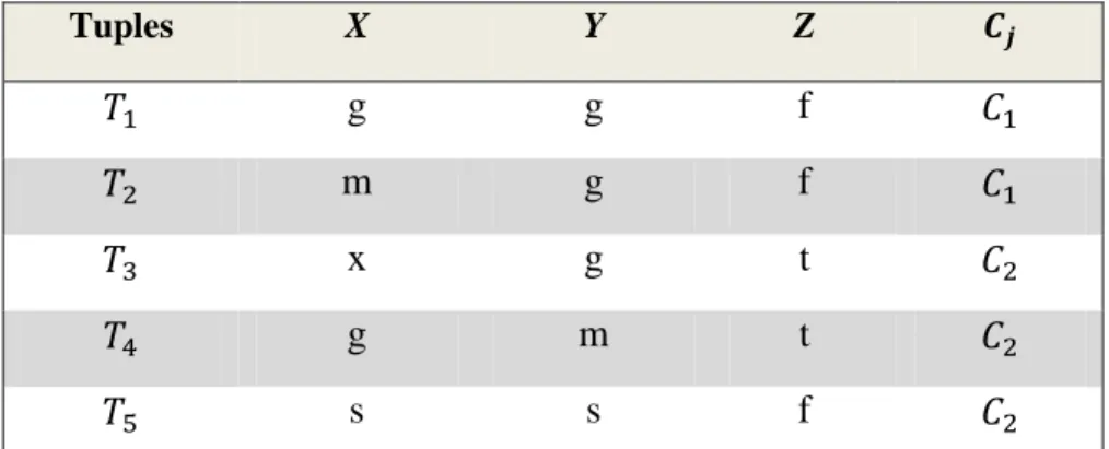
Table 2 represents a toy dataset which consists of 5 tuples represented by 4 attributes. Attributes X, Y, and Z represent the values from different domains and the fourth attribute represents the cluster ID to which the object belongs.

Table 2: A toy dataset

Tuples X Y Z g g f m g f x g t g m t s s f

For this dataset, * + and * +. Thus,

* + and * + are the centers for and , respectively. Now suppose that is a new object to be assigned to a cluster, and the given cohesion threshold is 0.60. Thus,

( ) ( )

and

( ) ( )

(44)

34

Intuitively, identical values in different domains could mean different things and assigned different weights. However, the CLUC’s similarity measure did not distinguish such differences by collecting categorical values as bags irrespective of the attributes they are representing. For instance, in Table 2, the value g (or m) occurring under the two attributes X and Y are considered and treated as identical. This problem is more serious when these identical values appear very frequently and under many different attributes. Such values usually negatively impact the importance of less frequent values which could be more important and meaningful. Most categorical clustering algorithms, including CLUC, considers categorical data types (nominal and binary) as one type and given them all equal weights. For example, attribute Z in Table 2 has two values and could be binary attributes, however, this attribute was treated similarly to the nominal attributes X and Y. We note that similar treatment of such attributes can result in poor clustering outputs. To illustrate this problem, consider the following collection of tuples in Table 3 for which we use CLUC to cluster.

Example 2:

Table 3: An instance of heart disease dataset

Tuple ID Gender Pain Types Smoker Fever Cough X-Ray Result

male normal yes no yes abnormal

female flat no yes yes normal

male sharp yes yes no indefinite

male normal no no no normal

male flat yes no no abnormal

female normal no no yes normal

Given Table 3 which includes two nominal attributes (Pain Type and X-Ray Result), and four binary attributes (Gender, Smoker, Fever, and Cough). In what follows, we present the steps of the clustering of this data, considering 0.6 as the cohesion parameter threshold.

(45)

35

 Initialization Phase:

1. is read, and since there is no cluster yet, is assigned to a new cluster and its center is

* +.

2. is read. Cohesion ( ) , so is assigned to and is updated with as:

* +.

3. is read. Cohesion ( ) , so is assigned to and is updated with as:

* +. 4. is read. Cohesion( ) , so is added to a new cluster with its cluster center

* +.

5. is read. Cohesion( ) . Cohesion( ) , so is assigned to and is updated with

as: * +

6. is read . Cohesion( ) . Cohesion( ) , so is assigned to and is updated with . * + .

To this point, two clusters were generated with four objects ( ) and with two objects ( )

 Refinement Phase

In this phase, the dataset is scanned repeatedly until no change in clusters.

1. is read . Cohesion( ) . Cohesion( ) , so is moved to . and are updated.

* +.

* +

2. is read. Cohesion( ) . Cohesion( ) , so is moved to and the centers are updated.

* + * +.

(46)

36

3. is read . Cohesion ( ) . Cohesion( ) . stays in . 4. is read. Cohesion ( ) . Cohesion( ) . stays in . 5. is read. Cohesion( ) . Cohesion ( ) . stays in . 6. is read. Cohesion( ) . Cohesion( ) . stays in .

Since two objects were moved, the dataset is scanned again:

1. is read. Cohesion ( ) . Cohesion( ) . stays in . 2. is read . Cohesion ( ) . Cohesion( ) . stays in . 3. is read . Cohesion ( ) . Cohesion( ) . stays in . 4. is read . Cohesion ( ) . Cohesion( ) . stays in . 5. is read . Cohesion ( ) . Cohesion( ) . stays in . 6. is read . Cohesion ( ) . Cohesion( ) . stays in

The clustering process is stopped here since no object moved between clusters. The final clustering result is shown in Table 4.

(47)

37

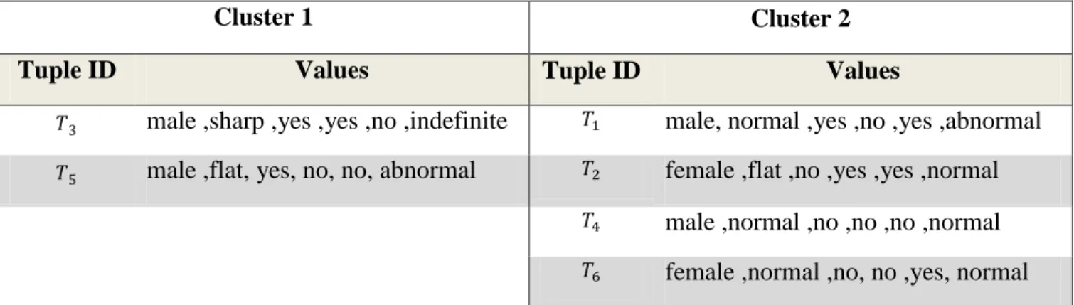
Table 4: CLUC clustering final result

Cluster 1 Cluster 2

Tuple ID Values Tuple ID Values

male ,sharp ,yes ,yes ,no ,indefinite male, normal ,yes ,no ,yes ,abnormal male ,flat, yes, no, no, abnormal female ,flat ,no ,yes ,yes ,normal

male ,normal ,no ,no ,no ,normal female ,normal ,no, no ,yes, normal

With and three times of iterations, CLUC‟s similarity measure partitions the dataset into two clusters: Cluster 1 with two objects and , and Cluster 2 with four objects , and . As pointed earlier, CLUC‟s similarity measure does not distinguish between the values in different domains which cause in increasing the weight of certain values and reducing the other. By looking at Table 4, it is clear that the clustering process was influencing by the two values “no” and “normal”. All the objects with these values were allocated into Cluster 1, although some should not be. For instance, is represented the case of a healthy patient which should be placed in a different cluster. However, because the value “no” appears three times in , it was assigned to cluster1. Similarly to , which represents the case of a patient with unusual test result that would be more reasonable to be isolated form other patients.

The problem of such measure arises when the given dataset is large and there are many asymmetric attributes. In many cases unimportant value such as “no” will get greater weight than “sharp” or “indefinite” that rarely appear. This affects negatively the quality and the interpretation of the clustering result.

(48)

38

4.2. Proposed Technique (

k-mixed

)

The main contribution of this thesis is the design of an effective algorithm, called k-mixed for clustering datasets with mixed attribute types. Given such a dataset, in the first step, called the discretization, the numeric values in the data are converted into discrete “categorical” values, using equal width method. In the second step, we use CLUC+, obtained by modifying the similarity measure of CLUC, a clustering method proposed for pure categorical data.

4.2.1 The

CLUC+

Algorithm

As pointed out in Section 4.1, we noted that the performance of the CLUC algorithm is negatively affected by two issues: (1) identical values that appear under different attributes, and (2) binary attributes. To overcome the shortcomings, we propose CLUC+, which addresses the first issue by labeling the attribute values with their attribute name (or number). This allows distinguishing between identical values under different attributes.

For the second issue on binary attributes, we propose to assign a greater weight to important and uncommon values, done in a similar way we assign weights to nominal values. That is, for symmetric attributes, both values are taken into account during the clustering process. For asymmetric attributes, rare values are considered to be important and hence assigned greater weights. In the same context, frequent values get small weights that is equal to 1. This strategy is (1) to ensure that different types do not contribute equally towards the clustering process, and (2) to prevent unimportant but high frequent values from dominating the clustering result.

To illustrate the idea, consider again Example 1 in Section 4.1. If we know that a binary attribute Z is asymmetric, then we can redefine the centers of clusters and as follows:

(49)

39

* + * +

and

* + * +

Here we describe how CLUC+ works. Consider a categorical dataset D which was divided by our proposed algorithm into k number of clusters. Each cluster has a center denoted by , which is an object represented by values of attributes in . Suppose that D has m categorical attributes which consist of nominal attributes, symmetric binary attributes, and asymmetric binary attributes. For this, we divided the values of these attributes into two categories: important values and less important values. Let us refer to the number of values of the first category as (ns) which includes: nominal values, symmetric binary values, and the rare values in the asymmetric attributes. The second category includes the most frequent values in the asymmetric attributes which we denote by (ab). Now if ( ) is the number of the different values of the attribute in , then the center is formed by two parts. One part represents the important values (ns), formed by the ( ) values for each attribute l with its frequency. The other part represents the less important values (ab), formed by listing their values. The cluster center is then constructed as:

* { } { } | + ( )

Using this, the cohesion between an objects and a cluster is then determined as:

( ) (∑ ∑ ) ( ⁄ ) ( ) where { ( ) ( ) ( ) ( ) and

(50)

40

{ ( ) ( ) ( )

It is important to note that there are two cases where asymmetric attributes are treated as nominal: 1. If the dataset is a pure binary dataset, then there is no biased treatment by our definition. 2. If the two values have the same frequency and we do not know which one is more important.

Let us consider again Example 2 in Section 4.1, and assume that attribute “Smoker” and “Cough” satisfy case 2 above, where we do not know which of the two {yes, no} values for attribute “Smoker” is more important. Likewise, for “Cough”, the number of occurrences of both values are the same. Then the clustering process proceeds as follows:

 Initialization Phase

1. The first item/object is read from the dataset and since no cluster has yet being created, , is assigned to a new cluster with its center as:

* + * +.

2. is read, and its cohesion to is calculated to be 0.16 . The cohesion is less than the given threshold value which was 0.60 so a new cluster is created with a center

* +

3. is read . Cohesion ( , ) = 0.33. Cohesion ( , )=0.0 , so creates a new cluster with a center * +

4. is read . Cohesion ( )= 0.16. Cohesion ( ) =0.50 . Cohesion ( )=0.33, so creates a new cluster with a center * + * +

An Efficient Technique for Clustering Data with Mixed Attribute Types