Declarative Probabilistic Programming with Datalog

(1)

Datalog

Vince Barany

1

, Balder ten Cate

2

, Benny Kimelfeld

3

, Dan Olteanu

4

,

and Zografoula Vagena

5

1 LogicBlox, Atlanta, GA, USA∗ 2 LogicBlox, Atlanta, GA, USA† 3 Technion, Haifa, Israel; and

LogicBlox, Atlanta, GA, USA

4 University of Oxford, Oxford, UK; and LogicBlox, Atlanta, GA, USA

5 LogicBlox, Atlanta, GA, USA

Abstract

Probabilistic programming languages are used for developing statistical models, and they typic-ally consist of two components: a specification of a stochastic process (the prior), and a specific-ation of observspecific-ations that restrict the probability space to a conditional subspace (the posterior). Use cases of such formalisms include the development of algorithms in machine learning and ar-tificial intelligence. We propose and investigate an extension of Datalog for specifying statistical models, and establish a declarative probabilistic-programming paradigm over databases. Our proposed extension provides convenient mechanisms to include common numerical probability functions; in particular, conclusions of rules may contain values drawn from such functions. The semantics of a program is a probability distribution over the possible outcomes of the input database with respect to the program. Observations are naturally incorporated by means of integrity constraints over the extensional and intensional relations. The resulting semantics is robust under different chases and invariant to rewritings that preserve logical equivalence.

1998 ACM Subject Classification D.1.6 Logic Programming, G.3 Probability and Statistics, H.2.3 Languages

Keywords and phrases Chase, Datalog, probability measure space, probabilistic programming

Digital Object Identifier 10.4230/LIPIcs.ICDT.2016.7

1 Introduction

Languages for specifying general statistical models are commonly used in the development of machine learning and artificial intelligence algorithms for tasks that involve inference under uncertainty. A substantial effort has been made on developing such formalisms and corresponding system implementations. An actively studied concept in that area is that ofProbabilistic Programming (PP) [20], where the idea is that the programming language allows for specifying general random procedures, while the systemexecutes the program not in the standard programming sense, but rather by means ofinference. Hence, a PP system is built around a language and an (approximate) inference engine, which typically makes use of Markov Chain Monte Carlo methods (e.g., the Metropolis-Hastings algorithm). The

∗ _{Now at Google, Inc.} † _{Now at Google, Inc.}

(2)

relevant inference tasks can be viewed as probability-aware aggregate operations over all possible worlds, that is, possible outcomes of the program. Examples of such tasks include finding the most likely possible world, or estimating the probability of an event. Recently, DARPA initiated the projectProbabilistic Programming for Advancing Machine Learning (PPAML), aimed at advancing PP systems (with a focus on a specific collection of systems, e.g., [40, 30, 32]) towards facilitating the development of algorithms and software that are based on machine learning.

In probabilistic programming, a statistical model is typically phrased by means of two components. The first component is agenerative process that produces a random possible world by straightforwardly following instructions with randomness, and in particular, sampling from common numerical probability functions; this gives theprior distribution. The second component allows to phrase constraints that the relevant possible worlds should satisfy, and, semantically, transforms the prior distribution into theposterior distribution– the subspace obtained by conditioning on the constraints.

As an example, in supervised text classification (e.g., spam detection) the goal is to classify a text document into one of several known classes (e.g., spam/non-spam). Training data consists of a collection of documents labeled with classes, and the goal of learning is to build a model for predicting the classes of unseen documents. One common approach to this task assumes a generative process that produces randomparameters for every class, and then uses these parameters to define a generator of random words in documents of the corresponding class [33, 31]. The prior distribution thus generates parameters and documents for each class, and the posterior is defined by the actual documents of the training data. Inunsupervised text classification the goal is to cluster a given set of documents, so that different clusters correspond to different topics (not known in advance). Latent Dirichlet Allocation [10] approaches this problem in a similar generative way as the above, with the addition that each document is associated with a distribution over topics.

A Datalog program is a set of logical rules, interpreted in the context of a relational database (where database relations are also called theextensional relations), that are used to define additional relations (known as theintensional relations). Datalog has traditionally been used as a database query language. In recent years, however, it has found new applications in data integration, information extraction, networking, program analysis, security, cloud computing, and enterprise software development [23]. In each of these applications, being declarative, Datalog makes specifications easier to write (sometimes with orders-of-magnitude fewer lines of code than imperative code, e.g., [28]), and to comprehend and maintain.

In this work, we extend Datalog with the ability to program statistical models. In par with existing languages for PP, our proposed extension consists of two parts: agenerative Datalog programthat specifies a prior probability space over (finite or infinite) sets of facts that we callpossible outcomes, and a definition of the posterior probability by means of

observations, which come in the form of ordinary logical constraints over the extensional and intensional relations. We subscribe to the premise of the PP community (and PPAML in particular) that this paradigm has the potential of substantially facilitating the development of applications that involve machine learning for inferring missing or uncertain information. Indeed, probabilistic variants are explored for the major programming languages, such as C [37], Java [27], Scala [40], Scheme [30] and Python [38] (we discuss the relationship of this work to related literature in Section 6). At LogicBlox, we are interested in extending our Datalog-based LogiQL [22] with PP to enable and facilitate the development of predictive analysis [6]. We believe that, once the semantics becomes clear, Datalog can offer a natural and appealing basis for PP, since it has an inherent (and well studied) separation between given data (EDB), generated data (IDB), and conditioning (constraints).

(3)

The main challenge, when attempting to extend Datalog with probabilistic programming constructs, is to retain the inherent features of Datalog. Specifically, the semantics of Datalog does not depend on the order by which the rules are resolved (chased). Hence, it is safe to provide a Datalog engine with the ability to decide on the chasing order that is estimated to be more efficient. Another feature is invariance under logical equivalence: two Datalog programs have the same semantics whenever their rules are equivalent when viewed as theories in first-order logic. Hence, it is safe for a Datalog engine to rewrite a program, as long as logical equivalence is preserved.

For example, consider an application where we want to predict the number of vis-its of clients to some local service (e.g., a doctor’s office). For simplicity, suppose that we have a schema with the following relations: LivesIn(person,city), WorksIn(person,employer), LocatedIn(company,city), and AvgVisits(city,avg). The following rule provides an appealing way to model the generation of a random number of visits for a person.

Visits(p,Poisson[λ])←LivesIn(p, c),AvgVisits(c, λ) (1) The conclusion of this rule involves sampling values from a parameterized probability distribution. Next, suppose that we do not have all the addresses of persons, and we wish to expand the simulation with employer cities. Then we might use the following additional rule.

Visits(p,Poisson[λ])←WorksIn(p, e),LocatedIn(e, c),AvgVisits(c, λ) (2) Now, it is not clear how to interpret the semantics of Rules (1) and (2) in a manner that retains the declarative nature of Datalog. If, for a personp, the right sides of both rules are true, should both rules “fire” (i.e., should we sample the Poisson distribution twice)? And ifpworks in more than one company, should we have one sample per company? And ifplives in one city but works in another, which rule should fire? If only one rule fires, then the semantics becomes dependent on the chase order. To answer these questions, we need to properly define what it means for the head of a rule to besatisfied when it involves randomness such asPoisson[λ].

Furthermore, consider the following (standard) rewriting of the above program. PersonCity(p, c)←LivesIn(p, c)

PersonCity(p, c)←WorksIn(p, e),LocatedIn(e, c) Visits(p,Poisson[λ])←PersonCity(p, c),AvgVisits(c, λ)

As a conjunction of first-order sentences, the rewritten program is equivalent to the previous one; we would therefore like the two programs to have the same semantics. In rule-based languages with a factor-based semantics, such asMarkov Logic Networks [15] orProbabilistic Soft Logic [11], the above rewriting may change the semantics dramatically.

We introduce PPDL, a purely declarative probabilistic programming language based on Datalog. The generative component of a PPDL program consists of rules extended with constructs to refer to conventional parameterized numerical probability functions (e.g., Poisson, geometrical, etc.). Specifically, these mechanisms allow sampling values from the given parameterized distributions in the conclusion of a rule (and if desired, use these values as parameters of other distributions). In this paper, our focus is on discrete numerical distributions (the framework we introduce admits a natural generalization to continuous distributions, such as Gaussian or Pareto, but we defer the details of this to future work). Semantically, a PPDL program associates to each input instanceI a probability distribution overpossible outcomes. In the case where all the possible outcomes are finite, we get a discrete probability distribution, and the probability of a possible outcome can be defined immediately

(4)

from its content. But in general, a possible outcome can be infinite, and moreover, the set of all possible outcomes can be uncountable. Hence, in the general case we obtain a probability measure space. We define a natural notion of aprobabilistic chase where existential variables are produced by invoking the corresponding numerical distributions. We define a measure space based on a chase, and prove that this definition is robust, in the sense that the same probability measure is obtained no matter which chase order is used.

A short version of this paper has appeared in the 2015 Alberto Mendelzon International Workshop [47].

2 Preliminaries

In this section we give basic notation and definitions that we use throughout the paper.

Schemas and instances. A (relational)schema is a collectionS ofrelation symbols, where each relation symbol R is associated with an arity, denoted arity(R), which is a natural number. Anattributeof a relation symbolRis any number in{1, . . . ,arity(R)}. For simplicity, we consider here only databases over real numbers; our examples may involve strings, which we assume are translatable into real numbers. Afact over a schemaS is an expression of the formR(c1, . . . , cn) whereRis an n-ary relation inS andc1, . . . , cn∈R. Aninstance I over

S is a finite set of facts overS. We denote byRI _{the set of all tuples (}_c

1, . . . , cn) such that

R(c1, . . . , cn)∈I.

Datalog programs. PPDL extends Datalog without the use of existential quantifiers. How-ever, we will make use of existential rules indirectly in the definition of the semantics. For this reason, we review here Datalog as well as existential Datalog. Formally, anexistential Datalog program, or Datalog∃ program, is a tripleD= (E,I,Θ) where: (1)E is a schema, called the extensional database (EDB) schema, (2) I is a schema, called the intensional database (IDB) schema, disjoint from E, and (3) Θ is a finite set of Datalog∃ rules, that is,

first-order formulas of the form∀x

(∃yψ(x,y))←ϕ(x)

whereϕ(x) is a conjunction of atomic formulas overE ∪ I andψ(x,y) is an atomic formula overI, such that each variable inxoccurs inϕ. Here, by anatomic formula (or,atom) we mean an expression of the form

R(t1, . . . , tn) whereR is ann-ary relation andt1, . . . , tn are either constants (i.e., numbers) or variables. For readability’s sake, we omit the universal quantifier and the parentheses around the conclusion (left-hand side), and write simply ∃yψ(x,y) ← ϕ(x). Datalog is the fragment of Datalog∃ where the conclusion of each rule is an atomic formula without existential quantifiers.

LetD= (E,I,Θ) be a Datalog∃ program. Aninput instance forDis an instance Iover

E. AsolutionofIw.r.t.Dis a possibly infinite setF of facts overE ∪ I, such thatI⊆F and

F satisfies all rules in Θ (viewed as first-order sentences). Aminimal solution ofI (w.r.t.D) is a solutionF ofIsuch that no proper subset of F is a solution of I. The set of all, finite and infinite, minimal solutions ofI w.r.t.D is denoted bymin-solD(I), and the set of all finiteminimal solutions is denoted by min-solfin_D(I). It is a well known fact that, ifD is a

Datalog program (that is, without existential quantifiers), then every input instanceI has a unique minimal solution, which is finite, and thereforemin-solfin_D(I) =min-solD(I).

Probability spaces. We separately considerdiscrete andcontinuous probability spaces. We initially focus on the discrete case; there, a probability space is a pair (Ω, π), where Ω is a finite or countably infinite set, called thesample space, andπ: Ω→[0,1] is such that

(5)

P

o∈Ωπ(o) = 1. If (Ω, π) is a probability space, thenπis aprobability distributionover Ω.

We say that πis anumerical probability distribution if Ω⊆R. In this work we focus on

discrete numerical distributions.

A parameterized probability distribution is a function δ : Ω×Rk → [0,1], such that

δ(·,p) : Ω→[0,1] is a probability distribution for all p∈Rk. We usepardim(δ) to denote

the parameter dimensionk. For presentation’s sake, we may writeδ(o|p) instead of δ(o,p). Moreover, we denote the (non-parameterized) distributionδ(·|p) byδ[p]. An example of a parameterized distribution isFlip(·|p), where Ω is {0,1}, and for a parameter p∈[0,1] we haveFlip(1|p) =pandFlip(0|p) = 1−p. Another example isPoisson(·|λ), where Ω =N, and

for a parameterλ∈(0,∞) we havePoisson(x|λ) =λx_e−λ_/x_{!. In Section 7 we discuss the} extension of our framework to models that have a variable number of parameters, and to continuous distributions.

Let Ω be a set. Aσ-algebraover Ω is a collectionF of subsets of Ω, such thatF contains Ω and is closed under complement and countable unions. (Implied properties include that

F contains the empty set, and thatF is closed under countable intersections.) IfF0 _{is a}

nonempty collection of subsets of Ω, then the closure ofF0 _{under complement and countable}

unions is a σ-algebra, and it is said to be generated by F0_{. A} _{probability measure space}

is a triple (Ω,F, π), where: (1) Ω is a set, called thesample space, (2) F is a σ-algebra over Ω, and (3) π : F →[0,1], called a probability measure, is such thatπ(Ω) = 1, and

π(∪E) =P

e∈Eπ(e) for every countable setE of pairwise-disjoint elements ofF.

3 Generative Datalog

A Datalog program without existential quantifiers specifies how to obtain a minimal solution from an input instance by producing the set of inferred IDB facts. In this section we presentgenerative Datalog programs, which specify how to infer adistribution over possible outcomesgiven an input instance. In Section 5 we will complement generative programs with

constraints to establish the PPDL framework.

3.1 Syntax

The syntax of a generative Datalog program is defined as follows.

IDefinition 1(GDatalog[∆]). Let ∆ be a finite set of parameterized numerical distributions.

1. A ∆-term is a term of the formδ[[p1, . . . , pk]] whereδ∈∆ is a parameterized distribution withpardim(δ) =`≤k, and eachpi (i= 1, . . . , k) is a variable or a constant. To improve readability, we will use a semicolon to separate the first`arguments (corresponding to the distribution parameters) from the optional other arguments (which we will call the

event signature), as in δ[[p;q]]. When the event signature is empty (i.e., whenk=`), we writeδ[[p; ]].1

2. A ∆-atom in a schemaSis an atomic formulaR(t1, . . . , tn) withR∈ Sann-ary relation,

such that exactly one term ti (i = 1, . . . , n) is a ∆-term and the other terms tj are variables and/or constants.2

1 _Intuitively,_δ[[_p_;_q_{]] denotes a sample from the distribution}_δ(·|_p_{) where different samples are drawn for} different values of the event signatureq(cf. Example 2).

(6)

House id city NP1 Napa NP2 Napa YC1 Yucaipa Business id city NP3 Napa YC1 Yucaipa City name burglaryrate Napa 0.03 Yucaipa 0.01 AlarmOn unit NP1 YC1 YC2 Figure 1Input instanceIof the burglar example.

1. Earthquake(c,Flip[[0.01;Earthquake, c]]) ← City(c, r)

2. Unit(h, c) ← House(h, c)

3. Unit(b, c) ← Business(b, c)

4. Burglary(x, c,Flip[[r;Burglary, x, c]]) ← Unit(x, c),City(c, r)

5. Trig(x,Flip[[0.6;Trig, x]]) ← Unit(x, c),Earthquake(c,1)

6. Trig(x,Flip[[0.9;Trig, x]]) ← Burglary(x, c,1)

7. Alarm(x) ← Trig(x,1)

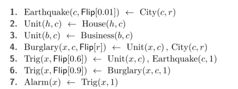
Figure 2GDatalog[∆] programG for the burglar example.

3. AGDatalog[∆]ruleover a pair of disjoint schemasE andI is a first-order sentence of the form ∀x(ψ(x)←φ(x)) where φ(x) is a conjunction of atoms inE ∪ I andψ(x) is either an atom inI or a ∆-atom inI.

4. AGDatalog[∆]program is a tripleG= (E,I,Θ), whereE andIare disjoint schemas and Θ is a finite set of GDatalog[∆] rules over E andI.

IExample 2. Our example is based on the burglar example of Pearl [39] that has been frequently used to illustrate probabilistic programming (e.g., [36]). Consider the EDB schema

E consisting of the following relations: House(h, c) represents houseshand their location citiesc, Business(b, c) represents businessesb and their location citiesc, City(c, r) represents citiesc and their associated burglary ratesr, and AlarmOn(x) represents units (houses or businesses)xwhere the alarm is on. Figure 1 shows an instance I over this schema. Now consider the GDatalog[∆] programG= (E,I,Θ) of Figure 2.

Here, ∆ consists of only one distribution, namelyFlip. The first rule in Figure 2, intuitively, states that, for every fact of the form City(c, r), there must be a fact Earthquake(c, y) where

y is drawn from the Flip (Bernoulli) distribution with the parameter 0.01. Moreover, the additional arguments Earthquake and c given after the semicolon (where Earthquake is a constant) enforce that different samples are drawn from the distribution for different cities (even if they have the same burglary rate), and that we never use the same sample as in Rules 5 and 6. Similarly, the presence of the additional argumentxin Rule 4 enforces that a different sample is drawn for a different unit, instead of sampling only once per city.

IExample 3. The program of Figure 3 models virus dissemination among computers of email users. For simplicity, we identify each user with a distinct computer. Every message has a probability of passing a virus, if the virus is active on the source. If a message passes the virus, then the recipient has the virus (but it is not necessarily active, e.g., since the computer has the proper defence). And every user has a probability of having the virus active on her computer, in case she has the virus. Our program has the following EDBs:

Message(m, s, t) contains message identifiers msent from the usersto the usert. VirusSource(x) contains the users who are known to be virus sources.

(7)

1. PassVirus(m,Flip[[0.1;m]]) ← Message(m, s, t),ActiveVirus(s,1)

2. HasVirus(t) ← PassVirus(m,1),Message(m, s, t)

3. ActiveVirus(x,Flip[[0.5;x]]) ← HasVirus(x)

4. ActiveVirus(x,1) ← VirusSource(x)

PassVirus,1 PassVirus,2

ActiveVirus,1 ActiveVirus,2

HasVirus,1

∗

Figure 3Program and dependency graph for the virus-dissemination example.

1. Earthquake(c,Flip[0.01]) ← City(c, r)

4. Burglary(x, c,Flip[r]) ← Unit(x, c),City(c, r)

5. Trig(x,Flip[0.6]) ← Unit(x, c),Earthquake(c,1)

6. Trig(x,Flip[0.9]) ← Burglary(x, c,1)

Figure 4Burglar program from Figure 2 modified to use syntactic sugar.

In addition, the following IDBs are used.

PassVirus(m, b) determines whether a messagempasses a virus (b= 1) or not (b= 0). HasVirus(x, b) determines whether userxhas the virus (b= 1) or not (b= 0).

ActiveVirus(x, b) determines whether userxhas the virus active (b= 1) or not (b= 0). The dependency graph depicted in Figure 3 will be used later on, in Section 3.4, when we further analyse this program.

Syntactic sugar. The syntax of GDatalog[∆], as defined above, requires us to always make explicit the arguments that determine when different samples are taken from a distribu-tion (cf. the argument c after the semicolon in Rule 1 of Figure 2, and the arguments

x, cafter the semicolon in Rule 4 of the same program). To enable a more succinct nota-tion, we use the following convention: consider a ∆-atom R(t1, . . . , tn) in which the i-th

argument, ti, is a ∆-term. Then ti may be written using the simpler notation δ[p], in which case it is understood to be a shorthand forδ[[p;q]] whereqis the sequence of terms

r, i, t1, . . . , ti−1, ti+1, . . . , tn. Here, r is a constant uniquely associated to the relation R.

Thus, for example, Earthquake(c,Flip[0.01]) ← City(c, r) is taken to be a shorthand for Earthquake(c,Flip[[0.01;Earthquake,2, c]]) ← City(c, r). Using this syntactic sugar, the pro-gram in Figure 2 can be rewritten in a notationally less verbose way, cf. Figure 4. Note, however, that the shorthand notation is less explicit as to describing when two rules involve the same sample vs. different samples from the same probability distribution.

3.2 Possible Outcomes

A GDatalog[∆] programG= (E,I,Θ) is associated with a corresponding Datalog∃program b

G= (E,I∆_,_Θ∆_{). The}_{possible outcomes}_{of an input instance}_I _w.r.t._G_{will then be minimal}

solutions of Iw.r.t.Gb. Next, we describeI∆ and Θ∆.

The schema I∆ _extends_I _{with the following additional relation symbols: for each}_δ_∈_∆

withpardim(δ) =kand for eachn≥0, we have a (k+n+ 1)-ary relation symbol Resultδ_n. These relation symbols Resultδn are called thedistributional relation symbols ofI∆, and the

(8)

1a. ∃y ResultFlip₂ (0.01,Earthquake, c, y) ← City(c, r)

1b. Earthquake(c, y) ← City(c, r),ResultFlip₂ (0.01,Earthquake, c, y)

4a. ∃y ResultFlip₃ (r,Burglary, x, c, y) ← Unit(x, c), City(c, r)

4b. Burglary(x, c, y) ← Unit(x, c),City(c, r),ResultFlip₃ (r,Burglary, x, c, y)

5a. ∃yResultFlip₂ (0.6,Trig, x, y) ← Unit(x, c),Earthquake(c,1)

5b. Trig(x, y) ← Unit(x, c),Earthquake(c,1),ResultFlip₂ (0.6,Trig, y, x)

6a. ∃yResultFlip₂ (0.9,Trig, x, y) ← Burglary(x, c,1)

6b. Trig(x, y) ← Burglary(x, c,1),ResultFlip₂ (0.9,Trig, x, y)

Figure 5The Datalog∃programGbfor the GDatalog[∆] programG of Figure 2.

other relation symbols ofI∆ _{(namely, those of} _I_{) are referred to as the}_ordinary _relation

symbols. Intuitively, a fact in Resultδn represents the result of a particular sample drawn fromδ(wherekis the number of parameters ofδandnis the number of optional arguments that form the event signature).

The set Θ∆_{contains all Datalog rules from Θ that have no ∆-terms. In addition, for every}

rule of the formψ(x)←φ(x) in Θ, whereψcontains a ∆-term of the formδ[[p;q]] withn=|q|, Θ∆contains the rules∃yResultδn(p,q, y)←φ(x) andψ0(x, y)←φ(x),Result

δ

n(p,q, y), where

ψ0 is obtained fromψby replacingδ[[p;q]] byy. Apossible outcomeis defined as follows.

IDefinition 4(Possible Outcome). LetI be an input instance for a GDatalog[∆] programG. Apossible outcome forI w.r.t.Gis a minimal solution F ofI w.r.t.Gb, such thatδ(b|p)>0 for every distributional fact Resultδ_n(p,q, b)∈F.

We denote the set of all possible outcomes ofIw.r.t.G by ΩG(I), and we denote the set of

all finite possible outcomes by Ωfin

G(I).

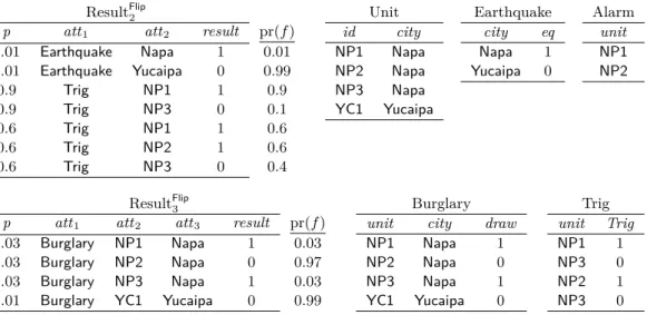
IExample 5. The GDatalog[∆] programG given in Example 2 gives rise to the Datalog∃ programGbof Figure 5. For instance, Rule 6 of Figure 2 is replaced with Rules 6a and 6b of Figure 5. An example of a possible outcome for the input instance I is the instance consisting of the relations in Figure 6 (ignoring the “pr(f)” columns for now), together with the relations ofI itself.

3.3 Probabilistic Semantics

The semantics of a GDatalog[∆] program is a function that maps every input instanceI to a probability distribution over ΩG(I). We now make this precise. For a distributional factf

of the form Resultδ_n(p,q, a), theprobabilityoff, denoted pr(f), is defined to beδ(a|p). For an ordinary (non-distributional) factf, we define pr(f) = 1. For a finite setF of facts, we denote byP(F) the product of the probabilities of all the facts inF:3

P(F)=def Y f∈F

pr(f)

3 _{The product reflects the law of total probability and does}_not_{assume that different random choices are} independent (and indeed, correlation is clear in the examples throughout the paper).

(9)

ResultFlip₂

p att1 att2 result pr(f)

0.01 Earthquake Napa 1 0.01 0.01 Earthquake Yucaipa 0 0.99 0.9 Trig NP1 1 0.9 0.9 Trig NP3 0 0.1 0.6 Trig NP1 1 0.6 0.6 Trig NP2 1 0.6 0.6 Trig NP3 0 0.4 Unit id city NP1 Napa NP2 Napa NP3 Napa YC1 Yucaipa Earthquake city eq Napa 1 Yucaipa 0 Alarm unit NP1 NP2 ResultFlip₃

p att1 att2 att3 result pr(f)

0.03 Burglary NP1 Napa 1 0.03 0.03 Burglary NP2 Napa 0 0.97 0.03 Burglary NP3 Napa 1 0.03 0.01 Burglary YC1 Yucaipa 0 0.99

Burglary

unit city draw

NP1 Napa 1 NP2 Napa 0 NP3 Napa 1 YC1 Yucaipa 0 Trig unit Trig NP1 1 NP3 0 NP2 1 NP3 0 Figure 6A possible outcome for the input instanceI in the burglar example.

I Example 6 (continued). Let J be the instance that consists of all of the relations in Figures 1 and 6. As we already remarked, J is a possible outcome of I w.r.t. G. For convenience, in the case of distributional relations, we have indicated the probability of each fact next to the corresponding row. P(J) is the product of all of the numbers in the columns titled “pr(f),” that is, 0.01×0.99×0.9× · · · ×0.99.

One can easily come up with examples where possible outcomes are infinite, and in fact, the space ΩG(I) of all possible outcomes is uncountable. Hence, we need to consider

probability spaces over uncountable domains; those are defined by means of measure spaces. Let G be a GDatalog[∆] program, and let I be an input forG. We say that a finite sequencef = (f1, . . . , fn) of facts is aderivation(w.r.t.I) if for alli= 1, . . . , n, the factfiis the result of applying some rule ofG that is not satisfied inI∪ {f1, . . . , fi−1} (in the case of applying a rule with a ∆-atom in the head, choosing a value randomly). If f1, . . . , fn is a derivation, then the set {f1, . . . , fn}is a derivation set. Hence, a finite setF of facts is a derivation set if and only ifI∪F is an intermediate instance in some chase tree.

LetGbe a GDatalog[∆] program,Ibe an input forG, andF be a set of facts. We denote by ΩF_G⊆(I) the set of all possible outcomes J ⊆ΩG(I) such that F ⊆ J. The following

theorem states how we determine the probability space defined by a GDatalog[∆] program.

I Theorem 7. Let G be a GDatalog[∆] program, and let I be an input for G. There exists a unique probability measure space (Ω,F, π), denoted µG,I, that satisfies all of the

following. 1. Ω = ΩG(I);

2. (Ω,F)is theσ-algebra generated from the sets of the formΩ_GF⊆(I)whereF is finite; 3. π(ΩF_G⊆(I)) =P(F)for every derivation setF.

Moreover, if J is a finite possible outcome, thenπ({J})is equal to P(J).

Theorem 7 provides us with a semantics for GDatalog[∆] programs: the semantics of a GDatalog[∆] programG is a map from input instancesIto probability measure spacesµG,I over possible outcomes (as uniquely determined by Theorem 7). The proof of Theorem 7 is by means of thechase procedure, which we discuss in the next section. A direct corollary of the theorem applies to the important case where all possible outcomes are finite (and the probability space may be infinite, but necessarily discrete).

(10)

I Corollary 8. Let G be a GDatalog[∆] program, and I an input instance for G, such that ΩG(I) = ΩfinG (I). Then P is a discrete probability function over ΩG(I); that is,

P

J∈ΩG(I)P(J) = 1.

3.4 Finiteness and Weak Acyclicity

Corollary 8 applies only when all solutions are finite, that is, ΩG(I) = ΩfinG (I). We now

present the notion ofweak acyclicity for a GDatalog[∆] program, as a natural syntactic condition that guarantees finiteness of all possible outcomes (for all input instances). This draws on the notion of weak acyclicity for Datalog∃[18]. Consider any GDatalog[∆] program

G= (E,I,Θ). Aposition ofI is a pair (R, i) whereR∈ I andiis an attribute ofR. The

dependency graph ofG is the directed graph that has the positions ofI as the nodes, and the following edges:

A normal edge (R, i)→(S, j) whenever there is a ruleψ(x)←ϕ(x) and a variablex

occurring at position (R, i) in ϕ(x), and at position (S, j) inψ(x). Aspecial edge (R, i)→∗₍_{S, j}_{) whenever there is a rule of the form} S(t1, . . . , tj−1, δ[[p;q]], tj+1, . . . , tn)←ϕ(x)

and a variablexoccurring at position (R, i) in ϕ(x) as well as in por q.

We say thatG isweakly acyclicif no cycle in its dependency graph contains a special edge.

ITheorem 9. If a GDatalog[∆]program G is weakly acyclic, then ΩG(I) = ΩfinG (I) for all input instancesI.

IExample 10. The burglar example program in Figure 2 is easily seen to be weakly acyclic (indeed, every non-recursive GDatalog[∆] program is weakly-acyclic). In the case of the virus-dissemination example, the dependency graph in Figure 3 shows that, although this program features recursion, it is weakly acyclic as well.

3.5 Discussion

We conclude this section with some comments. First, we note that the restriction of a conclusion of a rule to include a single ∆-term significantly simplifies the presentation, but does not reduce the expressive power. In particular, we could simulate multiple ∆-terms in the conclusion using a collection of predicates and rules. For example, if one wishes to have conclusion where a person gets both a random height and a random weight (possibly with shared parameters), then she can do so by deriving PersonHeight(p, h) and PersonWeight(p, w) separately, and using the rule PersonHW(p, h, w)←PersonHeight(p, h),PersonWeight(p, w). We also highlight the fact that our framework can easily simulate the probabilistic database model ofindependent tuples[46] with probabilities mentioned in the database. The framework can also simulate Bayesian networks, given relations that store the conditional probability tables, using the appropriate numerical distributions (e.g.,Flipfor the case of Boolean random variables). In addition, we note that adisjunctive Datalog rule [16], where the conclusion can be a disjunction of atoms, can be simulated by our model (with probabilities ignored): If the conclusion hasndisjuncts, then we construct a distributional rule with a probability distribution over{1, . . . , n}, and additionalndeterministic rules corresponding to the atoms.

4 Chasing Generative Programs

The chase[29, 3] is a classic technique used for reasoning about database integrity constraints such as tuple-generating dependencies. This technique can be equivalently viewed as a

(11)

tableaux-style proof system for ∀∗_∃∗_{-Horn sentences. In the special case of} _full

tuple-generating dependencies, which are syntactically isomorphic to Datalog rules, the chase is closely related to (a tuple-at-a-time version of) the naivebottom-up evaluation strategy for Datalog program (cf. [2]). We now present a suitable variant of the chase for generative Datalog programs, and use it in order to construct the probability space of Theorem 7.

We note that, although the notions and results could arguably be phrased in terms of a probabilistic extension of the bottom-up Datalog evaluation strategy, the fact that a GDatalog[∆] rule can create new values makes it more convenient to phrase them in terms of a suitable adaptation of the chase procedure.

Throughout this section, we fix a GDatalog[∆] program G= (E,I,Θ) and its associated Datalog∃programGb= (E,I∆,Θ∆). We first define the notions ofchase stepandchase tree. Chase step. Consider an instanceJ, a rule τ∈Θ∆_{of the form}_ψ₍_x₎_←_ϕ₍_x_{), and a tuple} a such thatϕ(a) is satisfied inJ butψ(a) is not satisfied inJ. Ifψ(x) is a distributional atom of the form∃yResultδ_i(p,q, y), thenψbeing “not satisfied” is interpreted in the logical sense (regardless of probabilities): there is noy such that (p,q, y) is in Resultδi. In that case, letJ be the set of all instancesJbobtained by extendingJ withψ(a) for a specific valuebof the existential variabley, such thatδ(b|p)>0. Furthermore, letπbe the discrete probability distribution overJ that assigns toJb the probability δ(b|p). Ifψ(x) is an ordinary atom without existential quantifiers,J is simply defined as{J0}, whereJ0 extendsJ with the fact

ψ(a), andπ(J0) = 1. We say thatJ−τ−−(a→) (J, π) is a valid chase step.

Chase tree. Let I be an input instance for G. A chase tree for I w.r.t.G is a possibly infinite tree, whose nodes are labeled by instances overE ∪ I, and whose edges are labeled by real numbers, such that:

1. The root is labeled byI;

2. For each non-leaf node labeled J, ifJ is the set of labels of the children of the node, and if πis the map assigning to each J0 ∈ J the label of the edge fromJ toJ0, then

J −τ−−(a→) (J, π) is a valid chase step for some ruleτ∈Θ∆ and tuplea.

3. For each leaf node labeledJ, there does not exist a valid chase step of the formJ −τ−−(a→)

(J, π). In other words, the tree cannot be extended to a larger chase tree.

We denote by L(v) the label (instance) of the node v. Each L(v) is said to be an

intermediate instancew.r.t. the chase tree. Consider a GDatalog[∆] programGand an input

I forG. Amaximal path of a chase treeT is a path P that starts with the root, and either ends in a leaf or is infinite. Observe that the labels (instances) along a maximal path form a chain (w.r.t. the set-containment partial order). A maximal pathP of a chase tree isfair

if whenever the premise of a rule is satisfied by some tuple in some intermediate instance onP, then the conclusion of the rule is satisfied for the same tuple in some intermediate instance onP. A chase treeT isfair (or has the fairnessproperty) if every maximal path is fair. Note that finite chase trees are fair. We restrict attention to fair chase trees. Fairness is a classic notion in the study of infinite computations;4_{moreover, fair chase trees can be}

constructed, for example, by maintaining a queue of “active rule firings.”

Let Gbe a GDatalog[∆] program,I be an input forG, andT be a chase tree. We denote bypaths(T) the set of maximal paths ofT. (Note thatpaths(T) may be uncountably infinite.) ForP ∈paths(T), we denote by∪P the union of the (chain of) labelsL(v) alongP.

(12)

ITheorem 11. LetG be a GDatalog[∆]program,I an input forG, andT a fair chase tree. The mappingP → ∪P is a bijection between paths(T)andΩG(I).

Chase measure. LetG be a GDatalog[∆] program, letI be an input forG, and letT be a chase tree. Our goal is to define a probability measure over ΩG(I). Given Theorem 11, we

can do that by defining a probability measure overpaths(T). A random path inpaths(T) can be viewed as aMarkov chain that is defined by a random walk overT, starting from the root. A measure space for such a Markov chain is defined by means ofcylindrification[7]. Letv

be a node ofT. The v-cylinder of T, denotedC_vT, is the subset of paths(T) that consists of all the maximal paths that containv. Acylinder ofT is a subset ofpaths(T) that forms av-cylinder for some nodev. We denote byC(T) the set of all the cylinders ofT.

Recall thatL(v) is a finite set of facts, and observe thatP(L(v)) is the product of the probabilities along the path from the root tov. The following theorem is a special case of a classic result on Markov chains (cf. [7]).

ITheorem 12. Let G be a GDatalog[∆] program, let I be an input for G, and let T be a chase tree. There exists a unique probability measure (Ω,F, π) that satisfies all of the

following. 1. Ω =paths(T).

2. (Ω,F)is theσ-algebra generated from C(T). 3. π(CT

v) =P(L(v))for all nodesv ofT.

Theorems 11 and 12 suggest the following definition.

IDefinition 13(Chase Probability Measure). LetG be a GDatalog[∆] program, letI be an input forG, letT be a chase tree, and let (Ω,F, π) be the probability measure of Theorem 12. The probability measureµT over ΩG(I) is the one obtained from (Ω,F, π) by replacing every

maximal pathP with the possible outcome∪P.

The following theorem states that the probability measure space represented by a chase tree is independent of the specific chase tree of choice.

ITheorem 14. LetG be a GDatalog[∆]program, letI be an input forG, and letT and T0 be two fair chase trees. Then µT =µT0.

5 Probabilistic-Programming Datalog

To complete our framework, we defineprobabilistic-programming Datalog,PPDL for short, wherein a program augments a generative Datalog program with constraints; these constraints unify the traditionalintegrity constraints of databases and the traditionalobservations of probabilistic programming.

IDefinition 15 (PPDL[∆]). Let ∆ be a finite set of parameterized numerical distributions. APPDL[∆]program is a quadruple (E,I,Θ,Φ), where (E,I,Θ) is a GDatalog[∆] program and Φ is a finite set of logical constraints overE ∪ I.5

I Example 16. Consider again Example 2. Suppose that we have the EDB relations ObservedHAlarm and ObservedBAlarm that represent observed home and business alarms, respectively. We obtain from the program in the example a PPDL[∆]-program by adding the following constraints:

(13)

1. ObservedHAlarm(h)→Alarm(h)

2. ObservedBAlarm(b)→Alarm(b)

We use right (in contrast to left) arrows to distinguish constraints from ordinary Datalog rules. Note that a possible outcomeJ of an input instanceIsatisfies these constraints if J

contains Alarm(x) for all x∈ObservedHAlarmI∪ObservedBAlarmI.

A PPDL[∆] program defines the posterior distribution over its GDatalog[∆] program, conditioned on the satisfaction of the constraints. A formal definition follows.

Let P = (E,I,Θ,Φ) be a PPDL[∆] program, and let G be the GDatalog[∆] program (E,I,Θ). Aninput instance forP is an input instanceIforG. We say thatIis alegal input instance if {J ∈ΩG(I)|J |= Φ} is a measurable set in the probability spaceµG,I, and its

measure is nonzero. Intuitively,Iis legal if it is consistent with the observations (i.e., with the constraints in Φ), givenG. The semantics of a PPDL[∆] program is defined as follows.

IDefinition 17. LetP = (E,I,Θ,Φ) be a PPDL[∆] program,G the GDatalog[∆] program (E,I,Θ),Ia legal input instance forP, andµG,I = (ΩG(I),FG, πG). The probability space

defined byP andI, denotedµP,I, is the triple (ΩP(I),FP, πP) where: 1. ΩP(I) ={J ∈ΩG(I)|J |= Φ}

2. FP ={S∩ΩP(I)|S∈ FG}

3. πP(S) =πG(S)/πG(ΩP(I)) for everyS∈ FP.

In other words,µP,I isµG,I conditioned on Φ.

I Example 18. Continuing Example 16, the semantics of this program is the posterior probability distribution that is obtained from the prior of Example 2, by conditioning on the fact that Alarm(x) holds for allx∈ObservedHAlarmI∪ObservedBAlarmI. Similarly, using an additional constraint we can express the condition that an alarm is off unless observed. One can ask various natural queries over this probability space of possible outcomes, such as the probability of the fact Earthquake(Napa,1).

We note that when Gis weakly acyclic, the event defined by Φ is measurable (since in that case the probability space is discrete) and the definition of legality boils down to the existence of a possible outcome.

5.1 Invariance under First-Order Equivalence

PPDL[∆] programs are fully declarative in a strong sense: syntactically their rules and constraints can be viewed as first-order theories. Moreover, whenever two PPDL[∆] programs, viewed in this way, are logically equivalent, then they are equivalent as PPDL[∆] programs, in the sense that they give rise to the same set of possible outcomes and the same probability distribution over possible outcomes.

Formally, we say that two PPDL[∆] programs,P1= (E,I,Θ1,Φ1) andP2= (E,I,Θ2,Φ2),

aresemantically equivalentif, for all input instancesI, the probability spacesµP1,I andµP2,I

coincide. Syntactically, the rules and constraints of a PPDL[∆] program can be viewed as a finite first-order theory over a signature consisting of relation symbols, constant symbols, and function symbols (here, if the same name of a function name is used with different numbers of arguments, such asFlip in Figure 2, we treat them as distinct function symbols). We say thatP1 andP2 areFO-equivalent if, viewed as first-order theories, Θ1 is logically equivalent

to Θ2 (i.e., the two theories have the same models) and likewise for Φ1 and Φ2. We have the

following theorems.

ITheorem 19. If two PPDL[∆]programs are FO-equivalent, then they are semantically equivalent (but not necessarily vice versa).

(14)

ITheorem 20. First-order equivalence is decidable for weakly acyclic GDatalog[∆]programs. Semantic equivalence is undecidable for weakly acyclic GDatalog[∆]programs (in fact, even for∆ =∅).

6 Related Work

Our contribution is a marriage between probabilistic programming and the declarative spe-cification of Datalog. The key features of our approach are the ability to express probabilistic modelsconcisely anddeclaratively in a Datalog extension with probability distributions as first-class citizens. Existing formalisms that associate a probabilistic interpretation with logic are either not declarative (at least in the Datalog sense) or depart from the probabilistic programming paradigm (e.g., by lacking the support for numerical probability distributions). We next discuss representative related formalisms and contrast them with our work. They can be classified into three broad categories: (1)imperative specifications over logical structures,

(2)logic over probabilistic databases, and (3)indirect specifications over the Herbrand base. (Some of these formalisms belong to more than one category.)

The first category includes imperative probabilistic programming languages [42]. We also include in this category declarative specifications of Bayesian networks, such as BLOG [32] and P-log [8]. Although declarative in nature, these languages inherently assume a form of acyclicity that allows the rules to be executed serially. Here we are able to avoid such an assumption since our approach is based on the minimal solutions of an existential Datalog program. The program in Figure 3, for example, uses recursion (as is typically the case for probabilistic models in social network analysis). In particular, it is not clear how this program can be phrased by translation into a Bayesian network. BLOG can express probability distributions over logical structures, via generative stochastic models that can draw values at random from numerical distributions, and condition values of program variables on observations. In contrast with closed-universe languages such as SQL and logic programs, BLOG considers open-universe probability models that allow for uncertainty about the existence and identity of objects.

The formalisms in the second category view the generative part of the specification of a statistical model as a two-step process. In the first step, facts are randomly generated by a mechanism external to the program. In the second step, a logic program, such as Prolog [26] or Datalog [1], is evaluated over the resulting random structure. This approach has been taken by PRISM [44], theIndependent Choice Logic[41], and to a large extent byprobabilistic databases [46] and their semistructured counterparts [25]. We focus on a formalism that completely defines the statistical model, without referring to external processes. As an important example, in PPDL one can sample from distributions that have parameters that by themselves are randomly generated using the program. This is the common practice in Bayesian machine learning (e.g., logistic regression), but it is not clear how it can be done within approaches of the second category.

One step beyond the second category and closer to our work is taken by uncertainty-aware query languages for probabilistic data such as TriQL [48], I-SQL, and world-set algebra [4, 5]. The latter two are natural analogs to SQL and relational algebra for the case of incomplete information and probabilistic data [4]. They feature constructs such asrepair-key, choice-of,possible, and group-worlds-bythat can construct possible worlds representing all repairs of a relation w.r.t. key constraints, close the possible worlds by unioning or intersecting them, or group the worlds into sets with the same results to sub-queries. World-set algebra has been extended to (world-set) Datalog, fixpoint, and

(15)

while-languages [14] to define Markov chains. While such languages cannot explicitly specify probability distributions, they may simulate a specific categorical distribution indirectly using non-trivial programs with specialized language constructs likerepair-keyon input tuples with weights representing samples from the distribution.

MCDB [24] and SimSQL [12] propose SQL extensions (with for-loops and probability distributions) coupled with Monte Carlo simulations and parallel database techniques for stochastic analytics in the database. Their formalism does not involve the semantic challenges that we have faced in this paper. Although being based on SQL, these extensions do not offer a truly declarative means to specify probabilistic models, and end up being more similar to the imperative languages mentioned under the first category.

Formalisms in the third category use rule weighting as indirect specifications of probability spaces over theHerbrand base, which is the set of all the facts that can be obtained using the predicate symbols and the constants of the database. This category includesMarkov Logic Networks (MLNs)[15, 34], where the logical rules are used as a compact and intuitive way of definingfactors. In other words, the probability of a possible world is the product of all the numbers (factors) that are associated with the grounded rules that the world satisfies. This approach is applied in DeepDive [35], where a database is used for storing relational data and extracted text, and database queries are used for defining the factors of a factor graph. We view this approach asindirect since a rule does not determine directly the distribution of values. Moreover, the semantics of rules is such that the addition of a rule that is logically equivalent to (or implied by, or indeed equal to) an existing rule changes the semantics and thus the probability distribution. A similar approach is taken byProbabilistic Soft Logic[11], where in each possible world every fact is associated with a degree of truth.

Further formalisms in this category areprobabilistic Datalog[19],probabilistic

Datalog+/-[21], and probabilistic logic programming (ProbLog) [26]. There, every rule is associated with a probability. For ProbLog, the semantics is not declarative as the rules follow a certain evaluation order; for probabilistic Datalog, the semantics is purely declarative. Both semantics are different from ours and that of the other formalisms mentioned thus far. A Datalog rule is interpreted as a rule over a probability distribution over possible worlds, and it states that, for a given grounding of the rule, the marginal probability of being true is as stated in the rule. Probabilistic Datalog+/- uses MLNs as the underlying semantics. Besides our support for numerical probability distributions, our formalism is used for defining a single probability space, which is in par with the standard practice in probabilistic programming. As discussed earlier, GDatalog[∆] allows for recursion, and the semantics is captured by (possibly infinite) Markov chains. Related formalisms are that of Probabilistic Context-Free Grammars (PCFG) and the more general Recursive Markov Chains (RMC) [17], where the probabilistic specification is by means of a finite set of transition graphs that can call one another (in the sense of method calls) in a possibly recursive fashion. In the database literature, PCFGs and RMCs are used in the context of probabilistic XML [13, 9]. These formalisms do not involve numerical distributions. In future work, we plan to study their relative expressive power compared to restrictions of our framework.

7 Concluding Remarks

We proposed and investigated a declarative framework for specifying statistical models in the context of a database, based on a conservative extension of Datalog with numerical distributions. The framework differs from existing probabilistic programming languages not only due to the tight integration with a database, but also because of its fully declarative

(16)

rule-based language: the interpretation of a program is independent of transformations (such as reordering or duplication of rules) that preserve the first-order semantics. This was achieved by treating a GDatalog[∆] program as a Datalog program with existentially quantified variables in the conclusion of rules, and applying a suitable variant of the chase. This paper opens various important directions for future work. One direction is to establish tractable conditions that guarantee that a given input is legal. Also, an interesting problem is to detect conditions under which the chase is aself conjugate[43], that is, the probability spaceµP,I is captured by a chase procedure without backtracking.

Our ultimate goal is to develop a full-fledged PP system based on the declarative specification language that we proposed here. In this work we focused on the foundations and robustness of the specification language. As in other PP languages, inference, such as computing the marginal probability of an IDB fact, is a challenging aspect, and we plan to investigate the application of common approaches such as sampling-based and lifted-inference techniques. We believe that the declarative nature of PPDL can lead to identifying interesting fragments that admit tractable complexity due to specialized techniques, just as is the case for Datalog evaluation in databases.

Practical applications will require further extensions to the language. We plan to support continuous probability distributions (e.g., continuous uniform, Pareto, and Gaussian), which are often used in statistical models. Syntactically, this extension is straightforward: we just need to include these distributions in ∆. Likewise, extending the probabilistic chase is also straightforward. More challenging is the semantic analysis, and, in particular, the definition of the probability space induced by the chase. We also plan to extend PPDL to support distributions that take a variable (and unbounded) number of parameters. A simple example is thecategoricaldistribution where a single member of a finite domain of items is to be selected, each item with its own probability; in this case we can adopt therepair-key operation of the world-set algebra [4, 5]. Finally, we plan to add support formultivariate distributions, which are distributions with a support inRk fork >1 (where, again,k can be

variable and unbounded). Examples of popular such distributions are multinomial, Dirichlet, and multivariate Gaussian distribution.

At LogicBlox, we are working on extending LogiQL with PPDL. An interesting syntactic and semantic challenge is that a program should contain rules of two kinds: probabilistic programming (i.e., PPDL rules) and inference over probabilistic programs (e.g., find the most likely execution). The latter rules involve the major challenge of efficient inference over PPDL. Towards that, our efforts fall in three different directions. First, we implement samplers of random executions. Second, we translate programs of restricted fragments into external statistical solvers (e.g., Bayesian Network libraries andsequential Monte Carlo [45]). Third, we are looking into fragments where we can apply exact and efficient (lifted) inference.

Acknowledgments. We are thankful to Molham Aref, Todd J. Green and Emir Pasalic for insightful discussions and feedback on this work. We also thank Michael Benedikt, Georg Gottlob and Yannis Kassios for providing useful comments and suggestions. Benny Kimelfeld is a Taub Fellow, supported by the Taub Foundation. Kimelfeld’s work was supported in part by the Israel Science Foundation. Dan Olteanu acknowledges the support of the EPSRC programme grant VADA. This work was supported by DARPA under agreements #FA8750-15-2-0009 and #FA8750-14-2-0217. The U.S. Government is authorized to reproduce and distribute reprints for governmental purposes notwithstanding any copyright thereon.

(17)

References

1 Serge Abiteboul, Daniel Deutch, and Victor Vianu. Deduction with contradictions in Data-log. InICDT, pages 143–154, 2014.

2 Serge Abiteboul, Richard Hull, and Victor Vianu. Foundations of Databases. Addison-Wesley, 1995.

3 Alfred V. Aho, Catriel Beeri, and Jeffrey D. Ullman. The theory of joins in relational databases. ACM Trans. on Datab. Syst., 4(3):297–314, 1979.

4 Lyublena Antova, Christoph Koch, and Dan Olteanu. From complete to incomplete inform-ation and back. InSIGMOD, pages 713–724, 2007. doi:10.1145/1247480.1247559.

5 Lyublena Antova, Christoph Koch, and Dan Olteanu. Query language support for incom-plete information in the MayBMS system. InVLDB, pages 1422–1425, 2007.

6 Molham Aref, Balder ten Cate, Todd J. Green, Benny Kimelfeld, Dan Olteanu, Emir Pasalic, Todd L. Veldhuizen, and Geoffrey Washburn. Design and implementation of the LogicBlox system. InPDOS, pages 1371–1382. ACM, 2015.

7 Robert B. Ash and Catherine Doleans-Dade. Probability & Measure Theory. Harcourt Academic Press, 2000.

8 Chitta Baral, Michael Gelfond, and Nelson Rushton. Probabilistic reasoning with answer sets. Theory Pract. Log. Program., 9(1):57–144, 2009.

9 Michael Benedikt, Evgeny Kharlamov, Dan Olteanu, and Pierre Senellart. Probabilistic XML via Markov chains.PVLDB, 3(1):770–781, 2010.

10 David M. Blei, Andrew Y. Ng, and Michael I. Jordan. Latent dirichlet allocation. J. of Machine Learning Research, 3:993–1022, 2003.

11 Matthias Bröcheler, Lilyana Mihalkova, and Lise Getoor. Probabilistic similarity logic. In

UAI, pages 73–82, 2010.

12 Zhuhua Cai, Zografoula Vagena, Luis Leopoldo Perez, Subramanian Arumugam, Peter J. Haas, and Christopher M. Jermaine. Simulation of database-valued Markov chains using SimSQL. InSIGMOD, pages 637–648, 2013.

13 Sara Cohen and Benny Kimelfeld. Querying parse trees of stochastic context-free grammars. InICDT, pages 62–75. ACM, 2010.

14 Daniel Deutch, Christoph Koch, and Tova Milo. On probabilistic fixpoint and Markov chain query languages. InPODS, pages 215–226, 2010. doi:10.1145/1807085.1807114.

15 Pedro Domingos and Daniel Lowd. Markov Logic: An Interface Layer for Artificial Intel-ligence. Synthesis Lectures on AI and Machine Learning. Morgan & Claypool Publishers, 2009.

16 Thomas Eiter, Georg Gottlob, and Heikki Mannila. Disjunctive Datalog. ACM Trans. Database Syst., 22(3):364–418, 1997.

17 Kousha Etessami and Mihalis Yannakakis. Recursive Markov chains, stochastic grammars, and monotone systems of nonlinear equations.J. ACM, 56(1), 2009.doi:10.1145/1462153. 1462154.

18 Ronald Fagin, Phokion G. Kolaitis, Renée J. Miller, and Lucian Popa. Data exchange: Semantics and query answering. InICDT, pages 207–224, 2003.

19 Norbert Fuhr. Probabilistic Datalog: Implementing logical information retrieval for ad-vanced applications. JASIS, 51(2):95–110, 2000.

20 Noah D. Goodman. The principles and practice of probabilistic programming. InPOPL, pages 399–402, 2013.

21 Georg Gottlob, Thomas Lukasiewicz, MariaVanina Martinez, and Gerardo Simari. Query answering under probabilistic uncertainty in Datalog+/- ontologies. Annals of Math.& AI, 69(1):37–72, 2013. doi:10.1007/s10472-013-9342-1.

22 Terry Halpin and Spencer Rugaber.LogiQL: A Query Language for Smart Databases. CRC Press, 2014.

(18)

23 Shan Shan Huang, Todd Jeffrey Green, and Boon Thau Loo. Datalog and emerging ap-plications: An interactive tutorial. InSIGMOD, pages 1213–1216, 2011. doi:10.1145/ 1989323.1989456.

24 Ravi Jampani, Fei Xu, Mingxi Wu, Luis Leopoldo Perez, Christopher M. Jermaine, and Peter J. Haas. MCDB: a Monte Carlo approach to managing uncertain data. InSIGMOD, pages 687–700, 2008.

25 Benny Kimelfeld and Pierre Senellart. Probabilistic XML: models and complexity. In

Advances in Probabilistic Databases for Uncertain Information Management, volume 304 ofStudies in Fuzziness and Soft Computing, pages 39–66. Springer, 2013.

26 Angelika Kimmig, Bart Demoen, Luc De Raedt, Vitor Santos Costa, and Ricardo Rocha. On the implementation of the probabilistic logic programming language ProbLog. Theory and Practice of Logic Programming, 11:235–262, 2011. doi:10.1017/S1471068410000566.

27 Lyric Labs. Chimple. URL:http://chimple.probprog.org/.

28 Boon Thau Loo, Tyson Condie, Minos N. Garofalakis, David E. Gay, Joseph M. Heller-stein, Petros Maniatis, Raghu Ramakrishnan, Timothy Roscoe, and Ion Stoica. Declarative networking. Commun. ACM, 52(11):87–95, 2009.doi:10.1145/1592761.1592785.

29 David Maier, Alberto O. Mendelzon, and Yehoshua Sagiv. Testing implications of data dependencies. ACM Trans. on Datab. Syst., 4(4):455–469, 1979.

30 Vikash K. Mansinghka, Daniel Selsam, and Yura N. Perov. Venture: a higher-order prob-abilistic programming platform with programmable inference.CoRR, abs/1404.0099, 2014. URL:http://arxiv.org/abs/1404.0099.

31 Andrew Kachites McCallum. Multi-label text classification with a mixture model trained by EM. InAssoc. for the Advancement of Artificial Intelligence workshop on text learning, 1999.

32 B. Milch and et al. BLOG: Probabilistic models with unknown objects. InIJCAI, pages 1352–1359, 2005.

33 Kamal Nigam, Andrew McCallum, Sebastian Thrun, and Tom M. Mitchell. Text classific-ation from labeled and unlabeled documents using EM. Machine Learning, pages 103–134, 2000.

34 Feng Niu, Christopher Ré, AnHai Doan, and Jude W. Shavlik. Tuffy: Scaling up statistical inference in Markov Logic Networks using an RDBMS. PVLDB, 4(6):373–384, 2011.

35 Feng Niu, Ce Zhang, Christopher Re, and Jude W. Shavlik. DeepDive: Web-scale knowledge-base construction using statistical learning and inference. In Int. Workshop on Searching and Integrating New Web Data Sources, volume 884 ofCEUR Workshop Pro-ceedings, pages 25–28, 2012.

36 Aditya V. Nori, Chung-Kil Hur, Sriram K. Rajamani, and Selva Samuel. R2: an efficient MCMC sampler for probabilistic programs. InAAAI, pages 2476–2482, 2014.

37 Brooks Paige and Frank Wood. A compilation target for probabilistic programming lan-guages. InICML, volume 32, pages 1935–1943, 2014.

38 Anand Patil, David Huard, and Christopher J. Fonnesbeck. PyMC: Bayesian Stochastic Modelling in Python. J. of Statistical Software, 35(4):1–81, 2010.

39 Judea Pearl.Probabilistic reasoning in intelligent systems – networks of plausible inference. Morgan Kaufmann, 1989.

40 Avi Pfeffer. Figaro: An object-oriented probabilistic programming language. Technical report, Charles River Analytics, 2009.

41 David Poole. The independent choice logic and beyond. InProbabilistic Inductive Logic Programming – Theory and Applications, pages 222–243, 2008.

42 Repository on probabilistic programming languages, 2014. URL: http://www. probabilistic-programming.org.

(19)

43 H. Raiffa and R. Schlaifer. Applied Statistical Decision Theory. Harvard University Press, Harvard, 1961.

44 Taisuke Sato and Yoshitaka Kameya. PRISM: A language for symbolic-statistical modeling. InIJCAI, pages 1330–1339, 1997.

45 Adrian Smith, Arnaud Doucet, Nando de Freitas, and Neil Gordon.Sequential Monte Carlo methods in practice. Springer Science & Business Media, 2013.

46 Dan Suciu, Dan Olteanu, Christopher Ré, and Christoph Koch. Probabilistic Databases. Synthesis Lectures on Data Management. Morgan & Claypool Publishers, 2011.

47 Balder ten Cate, Benny Kimelfeld, and Dan Olteanu. PPDL: probabilistic programming with Datalog. In AMW, volume 1378 of CEUR Workshop Proceedings. CEUR-WS.org, 2015.

48 Jennifer Widom. Trio: a system for data, uncertainty, and lineage. In Charu Aggarwal, editor,Managing and Mining Uncertain Data, chapter 5. Springer-Verlag, 2008.