HAL Id: hal-02465807
https://hal-cnam.archives-ouvertes.fr/hal-02465807
Submitted on 4 Feb 2020
HAL
is a multi-disciplinary open access
archive for the deposit and dissemination of
sci-entific research documents, whether they are
pub-lished or not. The documents may come from
teaching and research institutions in France or
abroad, or from public or private research centers.
L’archive ouverte pluridisciplinaire
HAL
, est
destinée au dépôt et à la diffusion de documents
scientifiques de niveau recherche, publiés ou non,
émanant des établissements d’enseignement et de
recherche français ou étrangers, des laboratoires
publics ou privés.
A Label-based Edge Partitioning for Multi-Layer Graphs
Camelia Constantin, Cédric Du Mouza, Yifan Li
To cite this version:
Camelia Constantin, Cédric Du Mouza, Yifan Li. A Label-based Edge Partitioning for Multi-Layer
Graphs. 52nd Hawaii International Conference on System Sciences (HICSS 2019), Jan 2019, Maui,
Hawaii, United States. pp.2216-2225, �10.24251/HICSS.2019.269�. �hal-02465807�
A Label-based Edge Partitioning for Multi-Layer Graphs
Camelia Constantin LIP6, Sorbonne Universit´e, France
Cedric du Mouza CEDRIC, CNAM, France
Yifan Li
LIP6, Sorbonne Universit´e, France [email protected]
Abstract
Social network systems rely on very large underlying graphs. Consequently, to achieve scalability, most data analytics and data mining algorithms are distributed and graphs are partitioned over a set of servers. In most real-world graphs, the edges and/or vertices have different semantics and queries largely consider this semantics. But while several works focus on efficient graph computations on these “multi-semantic” graphs, few ones are dedicated to their partitioning. In this work, we propose a novel approach to achieve edge partitioning for multi-layer graphs, which considers both structural and edge-types (labels) localities. Our experiments on real life datasets with benchmark graph applications confirm that the execution time and the inter-partition communication can be significantly reduced with our approach.
1.
Introduction
Graph theory has been intensively studied in the past few centuries for solving real world problems in physics, biology, sociology and information systems. In particular, with the development of computer science, a number of data structures and algorithms have been developed to facilitate this calculation for a wide range of graph-related tasks from local telephone network design to components placement of an electronic circuit. However, the data stores created in last decades are becoming unexpectedly large especially in social media. For instance, Facebook has generated a massive social network with more than one billion users and hundreds of times more connections.
A solution to achieve scalability for analyzing and mining data is to partition the graph. In modern distributed computing systems, two main partition approaches for graph data are considered to scale to very large graphs: vertex partitionandedge partition. Recently, [1] demonstrated that the vertex-cut method outperforms edge-cut for distributed computation over
real world graphs, which are likely to have highly skew degree distribution. With respect to the workload balance status in a distributed computing context, it can improve the overall performance significantly.
Real life graph data often consists of different types of edges and/or vertices. Many graph computing tasks depend partly on this kind of information, like the recommendation calculation for given topics in social network, the community detection and analysis and the matching of regular expressions in labeled graph. However existing graph partitioning methods do not consider the heterogeneity structure of these graphs when allocating edges to the different servers. Naive approaches where the graph is split in several graphs, one per layer, lead either to vertices/edges redundancy or to unbalanced vertices/edges allocation. Additionally they require computations on different graphs so more communication and execution times. We believe that considering the edge/vertex heterogeneity when partitioning is essential to provide efficient computations by drastically reducing the communication between servers.
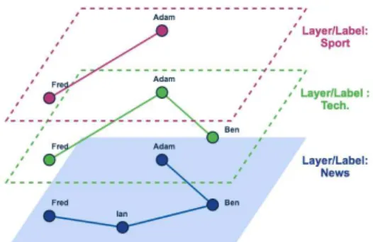
In this paper we consider aMulti-layer Graphmodel which assumes different types of connections, such as the Like/Follow/Friend interactions in social networks and/or the multi-labels on edge in user-interest graphs. Figure 1, represents an example of a 3-layer graph for a social network where we assume 3 topics: sport, technologyandnews. On the left-hand side, we have its representation as a single graph whose edges are multi-labeled. On the right-hand side we have its decomposition in three layers, i.e., three graphs, each one corresponding to a distinct label. Consequently to determinate recommendations for Adam on the topic news, we can run the recommendation algorithm on the according layer and not the complete multi-labeled graph. So the main contribution of our paper is a new edge partition method which enhances distributed graph computation by considering simultaneously the graph’s topology and its edge-semantics heterogeneity.
Figure 1. Multi-Layer Graph representations
introduction about multi-layer graph edge partitioning issue in Section 1, we present related work in Section 2. Then we introduce our block-based approach for graph partitioning using connectivity computation and block profiles in Section 3. We discuss about the seeds selection in Section 4 and block refinement and merging in Section 5. Experiments in Section 6 validate our approach. Finally Section 7 concludes the paper and gives perspectives.
2.
Related work
Numerous applications rely on graph exploitation, like online social network advertisement, public transportation optimization, or biological network analysis. In research, many efforts have been done on graph mining algorithms such as clustering, recommendation computation or pattern matching, by measuring topological properties, analyzing attributed contents,. . .. Nowadays it becomes crucial to find solutions to deal with current large graphs for maintaining those achievements from existing works. The natural way to achieve scalability is the classical strategy ”divide and rule”, and to the best of our knowledge, the initial work on this topic was Bulk Synchronous Parallel(BSP) model[2]. Later, the authors of [3] proposed METIS and its parallel implementation ParMETIS, which are a set of serial programs which allows graph partitioning based on the multilevel recursive-bisection, multilevel k-way, and multi-constraint partitioning schemes. Giraph [4] is another system developed, w.r.t the distributed graph processing, to help for easily implementing their applications over large graph in a parallel computing framework. More precisely, this work relies on Pregel model [5] by Google which converts the graph computation procedure into a sequence of iterations, namely supersteps, separated by global synchronization points. During each superstep, there is a common user-defined function executed on every vertex and the
messages will be sent/received by them to perform a specific graph algorithm, the processing will terminate when the graph reaches stable state which means no vertex is active. Almost at the same time, Low et al. proposed the GraphLab [6], an asynchronous shared-memory abstraction for distributed machine learning over graph data which is able to efficiently utilize memory of multiprocessors and get fast convergence for graph algorithms. All these proposals significantly improved the graph computations but the performance tends to degrade when the graph is particularly skewed, like the ones in social networks.
In [1], the new version of GraphLab, named PowerGraph, is proposed to overcome the limits of previous solutions for computing real life graphs which follow the highly skew degree distribution (power-law graphs). They introduced a new computation model named GAS that factors the vertex program along edges, to achieve the scalability of graph computation via partitioning graph data by edge instead of vertex. The graph processing module in Spark, GraphX[7], also employs a similar idea to GAS but provides more edge partitioning strategies to program developers.
In addition to their large scale, real graphs are also characterized by their heterogeneity. In other words, the vertices and edges in real world graphs usually have different types or attributes, which can largely impact the execution of graph algorithms deployed over them. While some recent works deal with heterogeneous network partitioning [8, 9] or clustering [10, 11], much additional efforts are still required to transfer vertex partitioning to edge partitioning, and to consider the relation between locality and label distribution has not been studied well. In [12], the authors present the C3Rframework to detect user communities based on
novel regularized spectral clustering approach that is able to perform an efficient partitioning of multi-layer user relations graph. But the time complexity of the framework, which is introduced by the graph Laplacians computation is a limit for real (very large) datasets.
Our approach is, to the best of our knowledge, the first one which achieves scalable edge partitioning for efficient querying on very large real multi-layer graphs.
3.
Block Construction
In a vertex-cut partitioning, i.e, edge partitioning, a vertex which belongs to several edges might be duplicated across partitions. In this Section, after introducing some definitions, we present how to allocate the different edges to limit the communication between a vertex and its replicated when processing a computation over a multi-graph.
Multi-layer graph.
Definition 1 (Multi-layer graph) A multi-layer graph is a tripleG(V, E,Λ)whereE ∈V ×V denotes a set of edges, V a set of vertices andΛ :E →2L\ ∅is the labeling function, withLthe domain of the edge labels. In other word, a multi-layer graph is a graph whose edges are labeled with one or more labels. Conceptually a multi-layer graph may be considered as a set of graphs, one for each label, which share the same vertices. We define the restriction of a multi-layer graphGto a given labellas:
Definition 2 (Multi-layer graph restriction) Let
G(V, E,Λ) be a multi-layer graph and a label
l ∈ dom(Λ). The restriction ofGtol, denotedGl, is
the graphGl(Vl, El)where
Vl⊆V ∧El⊆E∧ ∀e∈El, l∈Λ(e)
∧ ∀e′∈E\E
l, l /∈Λ(e′)
So the graphGlis the graph, possibly not-connected,
which contains all edges fromGlabeled withl. Block definition.
A block corresponds to a tightly knit cluster in graph, e.g. a community in social network. In our approach, we consider the block as a set of edges which are ”close” one to another, and these blocks become the component units of each partition in computation, but also the allocation units for workload over machines. More formally, a block is defined as follows.
Definition 3 (Block) Consider a graphG(V, E), a set S ⊆ V of vertices called seeds, and an allocation function alloc : E × S → boolean. A blockb is a couple(s, E′)wheres ∈ S is a node called theblock seedandE′ ⊆Eis a subset of edges such as∀e∈E′,
alloc(e, s) = trueand∀s′ ∈ S − {s}, alloc(e, s) =
f alse.
Theallocfunction allows to allocate an edge to the seed which is ”close”, considering both the topology (locality) and the labels (similarity). Consequently a block groups a set of edges close to each other in the graph and which share some common topics.
To take into consideration the locality of edges we propose aConnectivity Computation.
3.1.
Connectivity Computation
To preserve the locality inside a block, we adapt the Inverse P-distanceto capture the connectivity,i.e., closeness, from a seed to a given vertex. The idea is that the more paths there exist between two vertices and the shorter they are, the more connected (closer) these vertices are. We assume in the following that we have a directed graph but all the definitions work for a undirected graph with the associate semantics for paths and using the degree instead of the outdegree.
We compute the connectivity score conl v(i, j)
between vertexiandjfor a given labellin multi-layer graphG: conlv(i, j) = X p∈Pl ij S(pl) (1) where Pl
ij is the set of paths between i and j in the
multi-layer graph restrictionGl(i.e., the set ofl-labeled
paths in the multi-layer graph G), and S(pl) is the
inverse distance value calculated on pathpl,(v
0,v1, ..., vk)as: S(pl) = (1−α)k · k−1 Y i=0 1 outDegl(v i) (2) whereα∈(0,1)is the decay factor used in distance calculation, andoutDegl(v
i)is the number of out-edges
with labellfrom vertexvi.
Based on our vertex-to-vertex connectivity score we define an edge-to-vertex connectivity score which captures how ”close” an edge is from a given vertex. Definition 4 (Edge Connectivity) The connectivity score conl
e(k, e′) between a vertex k and an edge
e′ = (i, j)is: conl e(k, e′) =θ(con l v(k, i), con l v(k, j))
whereθis an aggregation function.
In the experiments we chose as the aggregate function the average function but any other aggregate function may be selected.
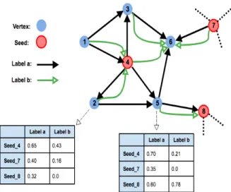
Figure 2. An example of connectivity scores calculation over multi-layer graph.
Example 1 Figure 2 depicts a 2-layer graph with labels aandb and three seeds (vertices 4, 7 and 8). For the vertices 2 and 5 we compute the connectivity scores to the different seeds for the different labels. For instance, considering the label a, we compute on the restrictionGathe connectivity scores between the vertex
2 and the seeds 4, 7 and 8. Assume (al edges are not depicted) that we get respectively the connectivity scorescona
v(v2, v4) = 0.65,conav(v2, v7) = 0.40and cona
v(v2, v8) = 0.32. Similar computation for the vertex 5 on Ga gives respectively the scores 0.70, 0.35 and
0.60. Consider the aggregateθ=avg, we obtain for the edgee2,5the edge connectivity scoresconea(v4, e2,5) =
1.35/2,cona
e(v7, e2,5) = 0.75/2andconae(v8, e2,5) =
0.92/2. Observe that we have some vertex connectivity scores equal to zero. It means that there exists no path between the vertex and the corresponding seed.
Since for each label, we have for each vertex (resp. edge) a score to each seed, we can adopt the following matrix representation.
Definition 5 (Connectivity Scores Matrices)
Consider the set S = {s1, s2, . . . , sκ} of seeds
and the setL = {l1, l2, . . . , lλ} of labels. The vertex
connectivity score matrix for a vertexk, denotedVk, is
a matrix with size|S| × |L|where
∀i∈[1..κ],∀j∈[1..λ], Vk(i, j) =conjv(k, si).
From this definition we can deduce the definition of the edge connectivity score matrixEǫ for an edgeǫ =
(k, k′)as:
∀i∈[1..κ],∀j ∈[1..λ], Eǫ(i, j) =θ(Vk(i, j), Vk′(i, j))
whereθis an aggregation function.
Observe that the computation of these two matrices can be implemented by performing a Breadth-First Search (BFS) from each seed in S for each label in
L, which can be easily deployed inPregel-like model systems. This computation has a time complexity of
O(|S| × |L| × (rq)), where |S| denotes the number
of seeds, |L| the number of labels and r the average degree of vertices, q corresponds to the depth of the BFS performed, generally a small value, e.g. 5in our experiments. In the matrixEǫeach column corresponds
to a label, and the highest score in a column points out the topologically closest seed for this edge in the corresponding graph restriction. However the candidate seed proposed for the edge allocation is likely to be different from one label to another. To determine the block to allocate the edge, we must consider all the labels in the same time. To achieve this, we first build a block profilefor the different blocks.
Example 2 Consider the example in Figure 2. The left table (resp. right table) corresponds to the matrix V2 of vertex2(resp. V5 of vertex5) for the seed setS =
{4,7,8} and the label set L = {a, b}. According to Definition 4, with the choice of addition as aggregation functionθ, we obtain the connectivity scores matrixEǫ
from the edgeǫ= (2,5)to every seed for each label in multi-layer graph: Eǫ= 1.35 0.64 0.75 0.16 0.92 0.78
We observe that for the labela (first column), the edgeǫgot the best score with seedS4while for the label bthe best score is obtained with seedS8.
3.2.
Block Profiles
The block profile is a summarization of the interests of the users within a block. Different content-based profiles for communities are proposed in literature like in [13, 14]. We propose a simple block profile construction based on the number of occurrences of the different labels of the edges of the block, but more advanced strategies may be used.
So assume that for the set of edgesE of a graphG
we have a setE′:{E
1, E2, ..., Ek}of blocks, such that
S
1≤i≤kEi ⊆Eand∀i,∀j, i6=j⇒Ei∩Ej=∅. Also
assume the existence of the functionocc: 2E× L →N
which returns the number of occurrences of a given label in a set of edges. We define the label score of a block as:
Definition 6 (label score of a block) The label score for a blockEand a labellis:
score(E, l) = P occ(E, l)
li∈Locc(E, li)
The block profile of a given block E consists of the set of the different label scores computed for each label l ∈ L = {l1, l2, . . . , lλ}. So we can represent
the different block profiles for a set of blocks E′ : {E1, E2, ..., Ek}as a matrixPthat we denote theblocks
profile matrix:
P = (pij)1≤i≤λ,1≤j≤kwith pij=score(Ei, lj)
Label correlation. The precedent definition assumes that the labels are independent one from another. In many applications, there exist however correlations between labels. For instance, we expect to group the edges (vertices) with labelsITandComputer together, or those with labelsPolitics andPolls, since they are more likely to be queried or processed concurrently in applications.
So we assume the existence of a correlation matrix of labels C(L) ∈ [0,1]|L|×|L|, with∀i,∀j, c
ij = cji
is the correlation score for label li with lj. Different
correlation functions exist to build this matrix like Pearson, Kendall or Spearman, for instance. Observe that if the different labels are independent the matrix
C(L)is equals to identity matrixI|L|2
.
Finally we adapt the definition of the block profile matrix to take into consideration the label correlation: Definition 7 (blocks profile matrix) Consider the set of blocksE′ : {E
1, E2, ..., Ek} and the set of labels
L = {l1, l2, . . . , lλ}, the blocks profile matrixPcorr is
the matrix
Pcorr=PT×C(L)
For the sake of simplicity, we use the notation P
instead ofPcorrin the following.
3.3.
Edge Allocation
Intuitively, starting a topic-based algorithm in a block with a small number of labels shared by its different edges will lead to less inter-block communication and consequently a faster execution time than a block with a large number of different labels with a uniform distribution. So our goal is to build such topic focusedblocks, which represent basically blocks of users sharing similar interests,i.e., a community. To
achieve this, we allocate an edge based on topology and on the different block’s profiles.
Proposition 1 (Edge allocation) Consider an edge ǫ
and blocks profile matrix P. ǫis allocated to the seed
sidetermined by:
argmaxx∈{1,...,|S|}{ax|ax∈A= (Eǫ⊙P)×1n}
where ⊙ denotes the entrywise product, and 1n is a
vector with all values to1.
Example 3 Assume in Figure 2 that labelsaandbare independent, and the blocks matrix profile P for the blocks corresponding to the seeds 4, 7 and 8 is:
0.8 0.2 0.75 0.25 0.5 0.5 ThenA= (Eǫ⊙P)×1nis: A= 1.35 0.64 0.75 0.16 0.92 0.78 ⊙ 0.8 0.2 0.75 0.25 0.5 0.5 · 1 1 = 1.35∗0.8 0.64∗0.2 0.75∗0.75 0.16∗0.25 0.92∗0.5 0.78∗0.5 · 1 1 = 1.208 0.6025 0.85
So from above result, edgee2,5should be allocated to the block associated to seed4.
4.
Seeds Selection
The choice of the seeds may largely impact the quality of the resulting partitioning since the edge allocation highly depends on the topological and thematic proximity of the seeds. While the seed selections is known as an NP-hard problem, we propose in the following a strategy with a linear complexity to select the seeds based on the topology and on the ”profiles” of the seeds.
We first propose theVariance of Edges,V OE(E′), to measure how the labels fromL are spread out over a set of edgesE′ ⊆ E. Intuitively, the more common edge labels and the fewer of them are involved, the higher V OE forE′. Formally, given a set of edges
E′ ⊆E, and set of labelsL∈ L,V OE(E′)is defined as the mean of the squared deviation from the mean of
label(E′)for each label inL:
PL
l (label
l(E′)−µ)2
wherelabell(E′)is number of edges having labell in edgesE′ andµ = PL
l label
l(E′)/|L|. Based on this measure, we can now propose criteria to select the seeds for our block construction.
Definition 8 (Seed) A vertexs∈V belongs to the seed setS, which satisfies:
i) ∀s′∈S, s /∈neighbor(s′)
ii) ∀v ∈ V \ S, β · DegL(s) + (1 − β) ·
V OE(adjacent(s))≥β·DegL(v) + (1−β)·
V OE(adjacent(v))
whereadjacent(x)denotes the set of edges with xas vertex, DegL(x) = P
l∈Llabel
l(adjacent(x))andβ
is an ad-hoc parameter in[0,1].
The first criterion avoids to select adjacent seeds which allows a better coverage of the large graph. Observe that we can decide to extend this criterion by requiring a distance of 2 or 3 between two seeds (but remember that recent results exhibit an average path length of 3.7 for Twitter [15]). The second criterion means that the seeds are selected among the most popular accounts (i.e., accounts with the largest number of labels on adjacent edges) but also those which federates a community around them with common/similar interest (i.e., labels), that will lead to a good block/partition construction. Indeed by selecting seeds with high degree and high VOE we expect to build dense blocks with a few number of distinct labels, leading to lower communication, thus processing time, when querying or mining the graph. Observe that the size of the seed set is a preset value, larger than the number of requested partitions.
We implemented the seed selection as a greedy algorithm presented in Algorithm 1. This algorithm has a linear complexity since it relies on a single scan of the list of vertices ordered by their degree. Consequently the number of vertices checked is comprised between |S|and|V|, where|S|denotes the size of the seed set.
The detailed procedure of selection is described in Algorithm 1. Example 4 illustrates the seed selection algorithm.
Example 4 Suppose we have a 2-layer graphG′, with labelsL = {a, b}, and 3 candidate seeds,{c1, c2, c3}, available. The statistics of labels on their adjacent edges are
(labela(adjacent(c
1)), labelb(adjacent(c1))) = (6,4), (labela(adjacent(c
2)), labelb(adjacent(c2))) = (2,6)and (labela(adjacent(c
3)), labelb(adjacent(c3))) = (4,4). Thus, we can calculate theDegL(c
i)of each candidate,
represented here as a vectordv = [6 + 4, 2 + 6, 4 + 4]T = [10, 8, 8]T. We normalize this scores and get
Algorithm 1:Seeds selection algorithm
input : the graphG(V, E), the set of labelsL
output : a set of seedsS
parameter: the number of seedsmand the importance factor of VOEβ
1 C← ∅; //the seed-candidates
2 N← ∅; //the neighbor vertices of existing candidates 3 while|C|< mdo
4 v=argmaxx∈V\NDeg(x); //the vertex with max
”Degree”
5 C+ ={v→(Deg(v), V OE(Adjacent(v)))}; 6 N+ =neighbor(v);
7 C′←norm(C); //we normalize the Deg() and VOE() values for elements inC
8 foreachc∈C′do 9 (deg, voe) =c.value() ;
10 c.valueUpdate(deg∗(1−β) +voe∗β) ;
11 S←C′.maxByValue(m); //to select the candidates with first m max values
12 ReturnS;
the vectordv′ = [10/26, 8/26, 8/26]T. At the same
time, theirV OEscan be figured out via formulas above. For instance, for c1, its V OE is ((6 − 5)2 + (4−
5)2)/2 = 1. We compute similarly the values for c 2 andc3and find4and0respectively. We also represent them as a vectorov = [1, 4, 0]. After normalization we get the vector ov′ = [1/5, 4/5, 0/5]T. We
assume in the following that the ad-hoc parameter β
is set to 0.5. We get consequently the finalsuitability score for each candidate, as(1−0.5)dv′+ 0.5ov′ =
[0.292, 0.554, 0.154]T. We conclude that candidatec
2 is most suitable for becoming a seed among these three candidates since it has the maximum value.
5.
Block Refinement and Merging
Our edge allocation algorithm ensures the construction of blocks which present a topic homogeneity but which may lead to a block size heterogeneity with small blocks or oppositely very large blocks. To make blocks fit the expected partition size we propose to proceed in two steps: first we split the oversized blocks into smaller ones and second we merge the different blocks to get the final partitioning.
For the first step, splitting a block into several sub-blocks (i.e., re-allocating edges to different sub-blocks) in a random way would reduce the benefit of our block constructions where locality and topic similarity were considered. So we propose to iterate recursively the edge allocation algorithm by selecting ⌈size(B)/max size block⌉seeds within the oversized block B. The block construction process stops when all blocks have a size lower than the given parameter
max size block.
Finally to get the final partitions and to respect their maximum size we perform block merging. Relying only
on block sizes to decide which blocks to merge (we call this strategy the 4/3 algorithm in the following) would result in partitions composed by sub-blocks topologically and/or thematically distant. So we propose to exploit the block locality to decide the blocks to merge. To achieve this we consider the block meta-graph, a weighted directed graph G′, where the vertexvi′ represents the blockbi and the weightwbi,sj
on edge e′
i,j is a vector which is the sum of edge
connectivity scores from every edge inbi to seedsj(of
block bj), in other words, ⊕e∈bi(E
e
ǫ)j, then we can
merge the blocks according to Algorithm 2.
Algorithm 2:Meta-Block allocation algorithm
input : A set of blocksBof sizen, a set of partitionsPof sizem, the labelsL, the partition maximal sizez
output : Each block is allocated to apj∈P
1 Initialization to avoid large blocks; 2 B′← ∅;
3 foreachbiin theBdo
4 bi.size←PLl labell(bi)
5 ifbi.size > zthen B′←B′∪split(bi) else
B′←B′∪b
i
6 whileB′6=∅do
7 pi=smallest(P)//retrieve the smallest partition;
8 V =B′.multiple(PL(p i), wbT
i,sj); //P L: blocks
profile matrix
9 b←largest(V); //to select the block with largest value in V
10 pi=merge(pi, b); //merge b with the smallest partition
11 B′=B′− {b}; 12 ReturnP;
Note that functions split() and merge() in Algorithm 2 correspond to the split and merge functions introduced earlier in this Section.
6.
Experiments
To evaluate our partitioning method on multi-layer graphs, we consider three graph-basic fundamental operations used in graph analysis and mining: Finding users with similar interest,Shortest PathsandRandom Walk, over our real-world datasets. We conduct the experiments on a Spark(1.6.1)[16] platform which is deployed on a 16 nodes cluster representing 100 cores. Observe that while the memory available allowed to store and handle our experimental datasets, we discard this centralized solution which was quickly outperformed by distributed solutions for our experiments. As the workload,i.e., the number of edges, is balanced between partitions for each partitioning strategies used in experiments, we focus on the runtime of each method to evaluate their performance.
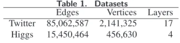
Table 1. Datasets
Edges Vertices Layers Twitter 85,062,587 2,141,325 17 Higgs 15,450,464 456,630 4
6.1.
Settings
Datasets
Two distinct datasets whose main features are summarized in Table 1 are used in our experiments:
TWITTER: An excerpt of Twitter with around 2
million vertices and 85 million edges corresponding to the sole f ollow links [17]. There exists a labell on an edge(u, v)to depict the interest of ufor the posts (tweets) of v on topicl. 17 labels are extracted from a supervised classification model to tag the different edges: leisure, technology, entertainment, labor, social, disaster, sport, life, environment, religion, law, politics, business, health, education, climate, war.
HIGGS[18] dataset built from the graph derived from Twitter during the discussions and interactions on the news of discovery of elusive Higgs boson on 4th July 2012. For this dataset no topic is considered but we distinguished 4 different interactions between users extracted in this graph and used to tag the edges: following, replying, mentioning and retweeting.
These datasets are large enough to illustrate the benefit of our partitioning approach. To handle larger graphs one may add more cluster nodes.
Competitors
We compare our algorithm with the most popular edge-partitioning algorithms, i.e. the ones proposed in GraphX and in PowerGraph. More precisely we compare the following partitioning strategies:
• Random edges allocation methods [7], such as RandomVertexCut, CanonicalRandomVertexCut, EdgePartition1D and EdgePartition2D.
• Greedy method introduced in PowerGraph [1]. • Our block-based method, esp., the Meta-Block
version has been employed in all following experiments as it always outperform 4/3 block allocationmethod (greedy block allocation). We choose to initially build ten times more blocks than the expected number of partitions.
6.2.
Finding user with similar interest
For the first experiment, we compare the impact of the partitioning strategies when performing the regular expression query (v, l,∗, l, x) which means we want to find all the vertices x which are connected to a given vertex by an edge with the same label l as v. This regular expression is a frequently-used query in graph mining operation [19] when we want to detect users x with similar interest l (whatever l may be) than user v. We run the different graph-partitioning algorithms to build partitionings with different sizes for each method. Then we conduct the regular expression query on these different partitionings and compare the resulting performances for 100,000 randomly selected vertices. Performance times correspond to total time (including pre-processing time).
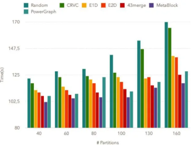
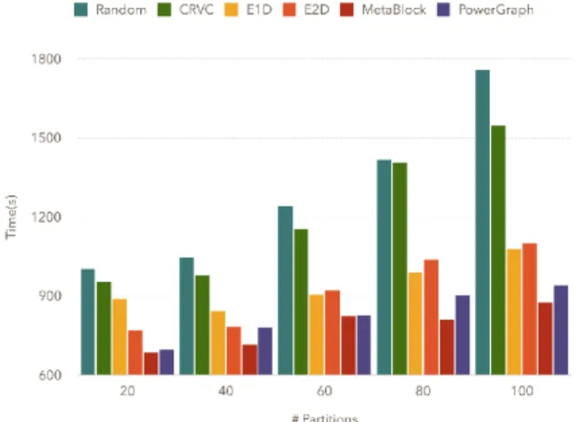
In Figure 3, we observe that for the Twitter graph the communication cost linearly increases with the number of partitions for all partitionings. However our partitioning strategy largely reduces the execution time. For instance with 100 partitions, we obtain a gain of 0.84, 0.3 and 0.33 for the random, EdgePartition2D or PowerGraph partitionings respectively.
We perform similar experiments with Higgs graph and results are depicted in Figure 4. Our method also outperforms existing ones for this dataset with a similar gain which enlightens that our approach remains efficient for graphs with a small number of distinct labels. Indeed, our partitions present a topic-homogeneity, so few distinct labels inside a partition, whatever the number of existing labels is. In plus we group edges based on topological proximity. Consequently the search for this regular expression on the graph is mainly processed within each partition, with few communication between partitions, whatever the size of the graph and/or the number of label are.
6.3.
Shortest Path
For this experiment we study the shortest path algorithm used in many applications such as community detection, influence or similarity computation, etc. Here, in our multi-graph assumption, we consider that ashortest path (SP)search corresponds to the following problem: for a graphG, given some landmarksΛ ⊆V
and a specific labelt, we want to find for every vertex
v ∈ V the shortest path to each reachable λ ∈ Λ
in the graph restriction Gt. The result of this search
is a vector of shortest path values to each landmark for each vertex. Observe that since the algorithm can be implemented using recursive search of neighbors (BFS), the implementation can be naturally deployed in
Figure 3. Regular expression query on Twitter graph
Figure 4. Regular expression query on Higgs graph
Figure 6. Shortest path on Higgs graph
Pregel-like systems, such as PowerGraph and GraphX. We construct 40-160 partitions for Twitter graph and we pick up a set of vertices randomly selected as landmarks (20 and 50 for respectively Twitter and Higgs datasets). The results are presented in Fig. 5. We notice that the runtime decreases from 10 to 60 percent, compared to other methods. The rationale is that our partitioning considers the connectivity and the labels for building blocks. So the resulting partitions usually present large subgraphs extracted from restriction graphs. Since the shortest paths are computed on the restricted graph of a chosen label, the computation is more likely to stay within a partition and thus reduces the communications between partitions. For the competitors the vertices which belong to the same restriction graph are allocated to much more partitions. So the vertex replication factor will be higher and more messages between partitions are required when performing a computation leading to higher runtimes. We make similar observations for the Higgs dataset (Fig. 6), so our partitioning strategy is also efficient for graphs with less labels.
6.4.
Random Walk
Random-walks are the building blocks for numerous widespread algorithms in different areas such as recommendation, similarity computation, item ranking or knowledge inference. In this Section, we conduct an experiment to illustrate how random walk-based algorithms may benefit from our partitioning algorithm. Algorithms on labeled graphs generally consider edge label as independent during the computation. However, the layers or labels of multi-graph are not independent in a variety of applications [20]. So we propose two types of random walk implementations for our experiments: 1)Independent-label Random Walks,where the random walks are conducted over only edge with queried label
λ,i.e., the graph restrictionGλ.
2)Correlated-label Random Walks, where we rely on the Correlation Matrix of Labels L, C(L), in Sec.3.3 into random walks execution. Thus the transitions for random walks consider all outgoing edges but with a weight which depends on the correlation between its label and the requested label. We choose here the Pearson correlation score, but other correlation scores may be investigate in the future. More precisely the transition probabilities are defined as:
P(vi→vj) = P(vi→vj|λ,C(L)) P ei,k∈EP(vi→vk|λ,C(L)) if ei,j∈E, 0 otherwise.
whereE is the edges of multi-layer graphG, λis the label to query and C(L) is the correlation matrix of labelsL. In above formula, we propose to calculate the overall probabilities of each transition via linearly summarizing all conditional ones. For the conditional probabilityP(vp → vq|λ, C(L), ep,q ∈ E), it can be estimated as: P(vp→vq|λ, C(L), ep,q∈E) = X l∈Labs(ep,q) Ck,t(L)
whereLabs(ep,q)is the set of labels for the edgeep,q.
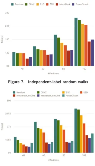
In Fig. 7, we see the benefit of our partitioning algorithm when performing independent-label random walks on Twitter dataset with a 30%-70% decrease for the runtime compared to executions on partitions produced by GraphX strategies, and around 5-10% decrease for GraphLab. The rationale is that with our partition building the random walk is likely to remain in the same partition since our partition algorithm considers graph distance and labels.
Fig. 8 presents the results for correlated-label random walks on Twitter dataset. We notice that our method, M etaBlock hasCM L, always provides the best execution times. The gain is even more important compared to independant-label random walks. This is due to our building which groups edges considering the topics and their correlation.
7.
Conclusion
In this paper, we present our approach for edge partitioning for multi-layer graphs which takes into account the locality of graph structure and the distribution of edge labels. We introduce new metrics, like Edge Connectivity Score and Blocks Profile Matrix, to determine the edge allocation. Our experiments
Figure 7. Independent-label random walks
Figure 8. Correlated-label random walks
on real-world datasets illustrate that the partitioning provided by our proposal allows different classical graph algorithms for graph analysis or graph mining to be executed much faster than when using another graph partitioning strategy.
As future work, we first intend to extend our proposal to support more complex graph models, where for instance the vertices also have different types of labels. We also plan to investigate a self-adaptive mechanism to determine the different parameters of our algorithm such as the number of seeds. Finally we intend to investigate the other kinds of relevant/valuable graph operations that our approach may improve.
References
[1] J. E. Gonzalez, Y. Low, H. Gu, D. Bickson, and C. Guestrin, “PowerGraph: Distributed Graph-parallel Computation on Natural Graphs,” inOSDI, pp. 17–30, 2012.
[2] L. G. Valiant, “A Bridging Model for Parallel Computation,” Commun. ACM, vol. 33, no. 8,
pp. 103–111, 1990.
[3] G. Karypis and V. Kumar, “A Fast and High Quality Multilevel Scheme for Partitioning Irregular Graphs,” SIAM J. Scientific Computing, vol. 20, no. 1, pp. 359–392, 1998.
[4] Apache, “Giraph.”http://giraph.apache.org, 2012.
[5] G. Malewicz, M. H. Austern, A. J. C. Bik, J. C. Dehnert, I. Horn, N. Leiser, G. Czajkowski, and G. Inc, “Pregel: A System for Large-scale Graph Processing,” inSIGMOD, pp. 135–146, 2010.
[6] Y. Low, D. Bickson, J. Gonzalez, C. Guestrin, A. Kyrola, and J. M. Hellerstein, “Distributed GraphLab: A Framework for Machine Learning and Data Mining in the Cloud,” Proc. VLDB Endow., vol. 5, no. 8, pp. 716–727, 2012.
[7] R. S. Xin, J. E. Gonzalez, M. J. Franklin, and I. Stoica, “GraphX: A Resilient Distributed Graph System on Spark,” inGRADES, pp. 2:1–2:6, 2013.
[8] D. Alistarh, J. Iglesias, and M. Vojnovic, “Streaming Min-max Hypergraph Partitioning,” in NIPS, pp. 1900–1908, 2015.
[9] K. Wei, R. Iyer, S. Wang, W. Bai, and J. Bilmes, “Mixed Robust/Average Submodular Partitioning: Fast Algorithms, Guarantees, and Applications,” in NIPS, pp. 2233–2241, 2015.
[10] J. Chen, W. Dai, Y. Sun, and J. Dy, “Clustering and Ranking in Heterogeneous Information Networks via Gamma-Poisson Model,” inICDM, pp. 424–432, 2015. [11] Y. Huang and X. Gao, “Clustering on Heterogeneous
Networks,”Wiley Int. Rev. Data Min. and Knowl. Disc., vol. 4, no. 3, pp. 213–233, 2014.
[12] A. Farseev, I. Samborskii, A. Filchenkov, and T. Chua, “Cross-Domain Recommendation via Clustering on Multi-Layer Graphs,” inSIGIR, pp. 195–204, 2017. [13] H. Fani, F. Zarrinkalam, E. Bagheri, and W. Du,
Time-Sensitive Topic-Based Communities on Twitter, pp. 192–204. Cham: Springer International Publishing, 2016.
[14] H. A. Abdelbary, A. M. ElKorany, and R. Bahgat, “Utilizing Deep Learning for Content-based Community Detection,” in 2014 Science and Information Conference, pp. 777–784, 2014.
[15] Q. Grossetti, C. Constantin, C. du Mouza, and N. Travers, “An Homophily-based Approach for Fast Post Recommendation in Microblogging Systems,” in
EDBT, (Wien, Austria), Mar. 2018.
[16] M. Zaharia, M. Chowdhury, T. Das, A. Dave, J. Ma, M. McCauly, M. J. Franklin, S. Shenker, and I. Stoica, “Resilient Distributed Datasets: A Fault-Tolerant Abstraction for In-Memory Cluster Computing,” in
NSDI, pp. 15–28, 2012.
[17] C. Constantin, R. Dahimene, Q. Grossetti, and C. du Mouza, “Finding Users of Interest in Micro-blogging Systems,” inEDBT, pp. 5–16, 2016. [18] M. De Domenico, A. Lima, P. Mougel, and M. Musolesi,
“The Anatomy of a Scientific Rumor,” vol. 3, pp. 2980 EP –, 10 2013.
[19] P. Barcel´o, L. Libkin, and J. L. Reutter, “Querying Graph Patterns,” inPODS, pp. 199–210, 2011.
[20] Y. Wang, X. Lin, and Q. Zhang, “Towards Metric Fusion on Multi-view Data: A Cross-view Based Graph Random Walk Approach,” inCIKM, pp. 805–810, 2013.