Data visualisation and exploration with prior knowledge

Data visualisation and exploration with prior

knowledge

Martin Schroeder, Dan Cornford, Ian T. Nabney Aston University, NCRG, Aston Triangle, Birmingham, B4 7ET, UK

[email protected]

Abstract. Visualising data for exploratory analysis is a major challenge in many applications where there is a need to gain insight into the structure and distribution of the data (e.g. to find common patterns and to identify relationships between samples as well as variables).

Typically, visualisation methods like principal components analysis (PCA) and multi-dimensional scaling (MDS) are employed.

These methods are favoured because of their simplicity but it is difficult to incorporate prior knowledge about properties of the variable space into the analysis (particularly important where strong correlations are present) or to cope with missing data.

One way to benefit from highly correlated variables is to model them us-ing a block correlation matrix; this reduces the number of free parame-ters significantly and also captures the structural knowledge. In this way, noise on the correlated variables is modelled with a common parame-ter. In this paper we show how to utilise on such information by us-ing a modification of a well known non-linear probabilistic visualisation model, Generative Topographic Mapping (GTM). The model has the ad-vantage it can cope with missing data, which is particularly valuable in high-dimensional sparse datasets.

In this paper it is shown that by including prior information about the grouping of variables in the covariance structure into the model one can improve both the data visualisation and the model fit. These benefits will be demonstrated on artificial data as well as a real geochemical dataset used for oil exploration, where the modification improved the imputation results by 3 to 13 %.

1

Introduction

Data visualisation is widely recognised as a key task in exploring and under-standing data sets. Including prior knowledge from experts into probabilistic models for data exploration is important since it constrains models, which usu-ally leads to more interpretable results and greater accuracy. As measurement becomes cheaper, datasets are becoming steadily higher dimensional. These

high-dimensional data sets pose a great challenge when using probabilistic models since the training time and the generalisation performance of these models depends on the number of free parameters.

A common fix for Gaussian models is to reduce the number of parameters and to ensure sparsity in the model by constraining the covariance matrix to be either diagonal, or spherical in the most restricted case. These constraints exclude valuable information about the data structure, especially in cases where there is some understanding of the structure of the covariance matrix.

A good example of this is data from chemical analysis like Gas Chromatography-Mass Spectrometry (GC-MS). When one examines the results of GC-MS runs over different samples, one knows that certain compounds are highly corre-lated with each other. This information can be incorporated into the model with a block-matrix covariance structure. This will help to reduce the number of free parameters without losing too much valuable information. In this paper we will look at a common probabilistic model for data exploration called the Gen-erative Topographic Mapping (GTM) [2]. The standard GTM uses a spherical covariance matrix and we will modify this algorithm to work with an informa-tive block covariance matrix.

The paper has the following structure. First we shortly review models for data visualisation and put them into context. Then we introduce the standard GTM model, extend it to the case of a block covariance matrix and describe how GTM can deal with missing data. Then we present some experiments on arti-ficial data and real data, where we compare the block version of GTM against spherical and full covariance versions and show where the advantages of the models lie. Finally we conclude the paper and point out further areas of re-search.

2

Data Exploration

A fundamental requirement for visualisation of high-dimensional data is to be able to map, or project, the high-dimensional data onto a low-dimensional rep-resentation (a ‘latent’space) while preserving as much information about the original structure in the high-dimensional space as possible.

There are many possible ways to obtain such a low-dimensional representa-tion. Context will often guide the approach, together with the manner in which the latent space representation will be employed. Some methods such as PCA and factor analysis [5] linearly transform the data space and project the data onto the lower-dimensional space while retaining the maximum information. Other methods like the Kohonen, or Self Organising, Maps [11] and the related Generative Topographic Mapping (GTM) [2, 1] try to capture the topology of the data. Another recent topology-preserving method, the Gaussian Process

Latent Variable Model (GP-LVM) [12] utilises a Gaussian Process prior over the mapping function. Instead of optimising the mapping function one consid-ers a space of functions given by the Gaussian Process. One then fits the model by directly optimising the positions of the point in the latent space. Geometry-preserving methods like multi-dimensional scaling [3] and Neuroscale [13] try to find a representation in latent space which preserves the geometric distances between the data points. The later approach can even be extended through a technique called Locally Linear Embedding [15, 9], which defines another met-ric to calculate the geometmet-ric distances, one used to optimise the mapping func-tion.

In this paper we will focus on the classical Generative Topographic Map-ping (GTM) and an extension which we will call Block Generative Topographic Mapping (B-GTM).

2.1 Standard GTM

The essence of GTM is to try to fit adensity model, which is constrained to lie on a 2-dimensional manifold, to the data in order to capture the structure in the high-dimensional data space. This manifold consists of a grid of points in the latent space which are connected via a non-linear mapping function to a distorted grid of Gaussian centres in the data space. Thus the GTM may be described as a mixture of Gaussians whose centres are constrained to lie on a manifold. To fit the intrinsic structure in the data, the non-linear mapping function is learned using an Expectation Maximisation (EM) algorithm [6] to maximise the data likelihood.

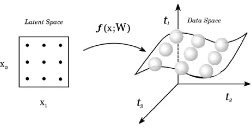
First one considers a functiont = f(x,W)which maps points x in theL -dimensional latent space into anL-dimensional non-Euclidean manifoldS em-bedded within theD-dimensional data space onto the pointst, shown for the caseL=2 andD=3 in Figure 2.1.

Defining a probability distribution p(x) for the data points in the latent space will induce a corresponding distribution p(t|W)in the data space con-sidering a mapping functiont = f(x,W). The conditional distribution oftis chosen to be a radially-symmetric Gaussian centered on f(x,W)with variance β−1. For a given value ofW, the distributionp(t|W)is obtained by integration over the distributionp(x)

p(t|W,β) =

Z

p(t|x,W,β)p(t)dx. (1)

A specific form of p(x)is considered, where p(x) is given by a sum of delta functions centred on the nodes of a regular grid in latent space

p(x) = 1 K K

∑

Fig. 1. The non-linear functionf(x,W)defines a manifoldSembedded in the data space given by the image of the latent variable space under the mappingx→t.

in which case the integral in (1) can be evaluated and and the corresponding log likelihood becomes

L(W,β) = N

∑

∑

To derive the EM algorithm for the GTM model, f(x,W)is chosen to be a linear-in-parameters regression model of the form f(x,W) =WΦ(x)with the elements ofΦ(x)consisting ofMfixed radial basis functions [4] andWbeing a D×Mmatrix. Formalising the EM algorithm one computes the responsibility, that each Gaussian generated the given data point in the E-Step:

Rin(Wold,βold) =p(xi|tn,Wold,βold) (4) = p(tn|xi,Wold,βold)

∑K

j=1p(tn|xj,Wold,βold). (5) Maximising the log likelihood one gets the updates forWandβin the M-step:

ΦT_G

oldΦWTnew=ΦTRT, (6) with Φ being a K×M matrix with elementsΦij = Φj(xi),Tbeing a N×D matrix with elements tnk,R being a K×Nmatrix with elements Rin and G being aK×Kdiagonal matrix with elements

Gii= N

∑

and forβ: 1 βnew = 1 ND N

∑

∑

A novel approach to include prior information about the correlations of vari-ables into the model is to use a full covariance matrix in the GTM noise model and to enforce a block structure onto it. This still results in a relatively sparse covariance matrix, keeping the number of unknown parameters at an accept-able level, while helping the model to fit the data including prior information about its structure. We assume that the groups of highly correlated variables are knowna priori. After ordering the variables by their known groups, the co-variance matrix will have the following structure:

Σ=       Σ1 0 . . . 0 0 Σ2 . .. ... .. . . .. ... 0 0 . . . 0 Σp       (9)

withΣ1toΣpbeing the submatrices of correlated group of variables. We further assume that there is no correlation between variables in distinct groups. The extension of the learning algorithm is straightforward since the only changes occur in the computation ofRin the E-step and ofΣin the M-step, where the calculation of the former is straightforward. For the M-step we have to derive the update for the full block covariance matricesΣb,b = 1, . . . ,p. Taking the derivative of the negative log likelihood with respect toΣbwe get:

Σ= 1 ND N

∑

∑

whereab_kn= (f(xk,W)b−tbn)withtbnbeing the pointtnonly at the dimensions for blockb.

2.3 Extension of GTM for Missing Data using EM

The EM algorithm can be used to estimate mixture model parameters in the presence of missing data[7]. This work has been extended to the GTM model [18] and it has been shown that the GTM performs quite well as an imputation method [16]. The extension for the block version of GTM is straightforward and will not be discussed here, but further details can be found in [17]

2.4 Stabilising the EM algorithm

A problem we encountered during the usage of the EM algorithm in conjunc-tion with the block and full GTM on high dimensional data was a collapse of the variance to very small values. This collapse was due to numerical errors when calculating the activation given by (4). The calculation of the activation involves a negative exponential term from the Gaussian, which in very high di-mensions becomes very small and thus gets truncated and substituted by 0 due to the limited precision of the floating point representation. This will ultimately result in points where the responsibility Rij is 0 for all Gaussians. The result is a collapse of the variance down to very small values, which in return leads to meaningless results in the projection. To prevent this from happening we use heuristics while calculating the activation as well as the covariance. These heuristics prevent the responsibilities for a data point from going to 0 for all the Gaussian kernels as well a collapse of the variance.

2.5 Assessing Unsupervised Learning

The dimensionality reduction methods discussed in this report are all examples of unsupervised learning. Thus we cannot tella prioriwhat is the expected or desired outcome. This makes it very difficult to judge which method is the best in the sense of telling us the most about a certain dataset. In the simple case of artificial data one can use prior knowledge about the structure of the data in the original space to quantify the error on the projection. For the more complex case of real data there are various approaches to this problem ranging from different resampling methods [19] to a Bayesian approach using the GP-LVM [8].

In this paper we are going to focus mainly on the following measures of the quality of a projection:

Nearest-Neighbour Label Error (NNLE): The nearest-neighbour label error can only be computed on labelled data, where we know the class of each data point. The idea is to consider the projected data and calculate for each point how many of theknearest points are in the same class. Then we average the fraction ofk -nearest neighbours in the same class over all the points. Finally we average over all the classes as well.

Missing Data or Data Resampling (RMSE): Another alternative approach we de-veloped is driven by the capabilities of the models to estimate missing data. Reestimating missing data can be seen as a resampling approach [14, 19] when the missing data patterns are created artificially and one retains the original value for comparison. Most probabilistic methods can be be modified to in-corporate assumptions about missing data. In the case where one introduces

missing data into the experiment after the model fit and where the model al-lows a back projection from the latent into the data space one can then use the model for data imputation. This way once can use missing data as benchmark method for these class of models. To benchmark the different methods against each other we are going to iteratively and piecewise delete every dimension d = 1, . . . ,Dfrom every point and see which estimates the model produce for the missing data. We then calculate the average root mean square error (RMSE) over all the points n = 1, . . . ,N, wheretare the original values and ˆtare the estimates: RMSE= 1 N N

∑

∑

3

Experiments On Artificial Data

To evaluate the effectiveness of block GTM (B-GTM) we carried out compar-ative experiments with spherical (i.e. standard) GTM (S-GTM), full GTM (F-GTM), and PCA. The data were sampled from a GTM with an 8×8 grid in the latent space. The grid was projected into a higher dimensional space using a 2×2 RBF. network. The weights were randomly sampled from a normal distri-bution with zero mean and unit standard deviation. Since the RBF was chosen with random weights the restriction to a 2×2 RBF ensured a non-linear but smooth and realistic mapping. The GTM used to generate the data had a block diagonal covariance matrix and experiments were conducted with a range of levels of variance and correlation. The overall variance of the data varied from 6.45 to 7.55, with covariances around the single Gaussians varying from 2 to 20, denoted by STD, in Figures 2 and 3. The amount of STD is in general controlls the amount of structure in the data. A low value for STD means now structure, while a high value means a lot of structure. In each experiment 100 data points were sampled from this GTM and each experiment was conducted 20 times, with a different randomly generated GTM each time.

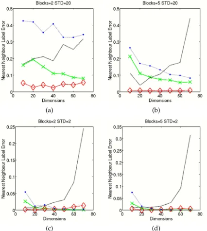
To calculate the NNLE the 8×8 grid was split into 4 classes with the 16 Gaussians in one corner of the grid being defined as one class. The results for this experiment, shown in Figure 2, indicate that in the case of little or no struc-ture in the data the B-GTM performs as well as, or only slightly worse than, S-GTM, while F-GTM is clearly struggling with increasing dimensionality. How-ever once more structure is present B-GTM clearly outperforms S-GTM, albeit once dimensionality increases the performance difference narrows. The differ-ence in number of blocks is significant as well since more blocks mean fewer pa-rameters for the B-GTM model. This results in improved performance as well.

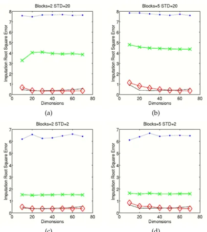
The RMSE was calculated on the same 20 projections. The results for this experiment, shown in Figure 3, indicate that the block as well as full version of

GTM always outperform the S-GTM regardless of the amount of block structure in the data. However the amount by which the spherical GTM is outperformed depends on the amount of block structure. Further there is no significant dif-ference between the performance of block or the full version of GTM. This can be explained due to the nature of imputation as a model validation technique, which only assess the fit of the model in the data space. If the GTM for example is warped on itself and thus gives poor results in the projection space, it will still give good imputation results if it properly covers the data cloud.

(a) (b)

(c) (d)

Fig. 2.The nearest neighbour label error on the artificial test data withhigh (STD=20) and low(STD=2) structure for the GTM model with different covariance structures. PCA=(blue, dotted line with big dot), S-GTM=(green, constant line with X), B-GTM=(red, slashed line with diamond), F-GTM=(black, slashed and dotted line)

(a) (b)

(c) (d)

Fig. 3.The root mean square error for imputation on the artificial test data withhigh (STD=20) and low(STD=2) structure for the GTM model with different covariance structures. PCA=(blue, dotted line with big dot), S-GTM=(green, constant line with X), B-GTM=(red, slashed line with diamond), F-GTM=(black, slashed and dotted line)

4

Experiments on Geochemical Data

To measure the performance of the projection methods for a real-world appli-cation domain we used a geochemical data set. The data set consists of 133 dif-ferent oil samples from the North Sea. The variables are peak heights from gas chromatograph-mass spectrometry featuring up to 61 different alkanes, ster-anes and hopster-anes. The data in the data sets have come from a variety of sources. It is normal in petroleum geochemistry, however, for the compound peaks of interest to be identified first, and then measured in height from top to bottom. The bottom is normally given by a realistic background signal (baseline). After the peak identification this is done by the software on the GC-MS system of the

source laboratory. As is standard in machine learning we pre-processed all vari-ables to have zero mean and unit variance. Since missing data are a common occurrence in geochemistry, we first excluded very sparse samples. Afterwards we excluded all non complete variables to obtain our complete data set with 61 remaining variables. Reasons for missing data include but are not exclusive to non performance of certain analysis due to cost savings, contaminated samples as well as errors in the peak detection.

% Missing 5 10 20 30 40 50 60 70

RMSE Improvement in % 0.04 0.13 0.03 0.04 0.13 0.10 0.10 0.04

Fig. 4.The overall improvement of performance in the RMSE from B-GTM to S-GTM

Using the data set, 20 random replications of missing data patterns for a given 0 < pi < 1 proportion of values missing were generated across all the variables. The patterns are chosen to be completely random, since we do not understand real missing data patterns sufficiently to reproduce them. Multiple Regression Imputation (MRI) [16] as well as mean imputation were chosen as benchmarks to evaluate how the models perform in general.

The apparently missing values are imputed using the GTM model and the Root Mean Square Error (RMSE) is used to assess the performance. The GTM models are all the same (3x3 RBF and 25x25 for the latent space) except for the covariance structure. In the case of the B-GTM the covariance block structure was chosen according to the input from geochemical experts.

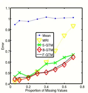
The results from the experiment indicate that the B-GTM with the informed block structure is superior to the GTM with a spherical and full covariance ma-trix as can be seen in Figure 4. The B-GTM consistently, and over a variety of missing data patterns, performs as well as or better than the F-GTM, while al-ways outperforming the normally-used spherical version of GTM. The gains in RMSE performance of B-GTM over S-GTM ranged on average between 3 and 13 % as can be see in the table in figure 4. The spread clearly shows that more random replications will be needed for smoother results, however these kinds of benchmarks are highly computational intensive and not the focus of this pa-per.

5

Conclusions

In this work we have introduced an extension to the GTM algorithm, which al-lows the user to specify a block structure for the covariance matrix. This block structure can either be the result from extensive data analysis, the inputs from

Fig. 5. The imputation root mean square error on North Sea Oil data. S=spherical, B=Block, F=Full

experts in the field and preferably a combination of both. The experiments show that the block extension is a beneficial to the GTM model if the data exhibit a certain amount of structure in the covariance matrix. When structure is present and correctly specified block GTM tends to perform at least as well as spherical or full GTM. In the case of the real geochemical data the gain from B-GTM over S-GTM ranged from 3 to 13 %. The RMSE also proved to be a helpful perfor-mance indicator, which however has to be treated with caution since one has to be aware that is only assess the fit of the model in the data space. The experi-ments further show that the assessment of unsupervised learning is a delicate task. One must understand the model behaviour as well as the restrictions of the model as well as the used performance indicators.

6

Future Work

Future work in this area will be aimed at assessing the possibility of including methods like Bayesian Correlation Estimation [10] into the algorithm in order to learn the correlation structure rather than rely on it being imposeda priori. Another approach might be the variational formulation of the GTM algorithm which includes the estimate of the correlation structure as well.

7

Acknowledgements

MS would like to thank the EPSRC and IGI Ltd. for funding his studentship un-der the CASE scheme. As well as the geochemical experts from IGI Ltd. (Chris Cornford, Paul Farrimond, Andy Mort, Matthias Keym) for their help and pa-tience.

References

1. C. M. Bishop, M. Svensen, and C. K. I. Williams. Gtm: a principled alternative to the self-organizing map.Artificial Neural Networks ? ICANN 96, pages 165–170, 1996. 2. C. M. Bishop, M. Svensen, and C. K. I. Williams. Developments of the generative

topographic mapping.Neurocomputing, 21:203–224, 1998.

3. I. Borg and P Groenen. Modern Multidimensional Scaling: theory and applications. Springer-Verlag New York, 2005.

4. D. Broomhead and D. Lowe. Feed-forward neural networks and topographic map-pings for exploratory data analysis. Complex Systems 2, pages 321–355, 1988. 5. C. Chatfield and A.J. Collins. Introduction to Multivariate Analysis. Chapman and

Hall, 1980.

6. A. Dempster, N. Laird, and D. Rubin. Maximum likelihood from incomplete data via the em algorithm. Journal of the Royal Statistical Society, Vol. 39:1–38, 1977. 7. Zoubin Ghahramani and Michael I. Jordan. Learning from incomplete data.

Tech-nical Report AIM-1509, 1994.

8. Stefan Harmeling. Exploring model selection techniques for nonlinear dimension-ality reduction. Technical report, Edinburgh University, Scotland, 2007.

9. V. de Silva J.B. Tenenbaum and J.C. Langford. A global geometric framework for nonlinear dimensionality reduction.Science, 290:2319–2323, 2000.

10. Merrill W. Liechty John C. Liechty and Peter Mller. Bayesian correlation estimation. Biometrika, 91:1–14, 2004.

11. T. Kohonen.Self-Organizing Maps. Springer Verlag, 1995.

12. Neil D. Lawrence. A scaled conjugate gradient algorithm for fast supervised learn-ing.Journal of Machine Learning Research 6, page 1783?1816, 2005.

13. D. Lowe and M.E. Tipping. Feed-forward neural networks and topographic map-pings for exploratory data analysis.Neural Computing and Applications, 4:84–95, 1996. 14. Ulrich Moeller and Doerte Radke. Performance of data resampling methods for robust class discovery based on clustering.Intelligent Data Analysis, 10:139?162, 2006. 15. S.T. Roweis and L.K. Saul. Locally linear embedding.Science, 290:2323–2326, 2000. 16. Martin Schroeder, Dan Cornford, Paul Farrimond, and Chris Cornford.

Address-ing missAddress-ing data in geochemistry: A non-linear approach. Organic Geochemistry, 39:1162–1169, 2008.

17. Martin Schroeder, Ian T. Nabney, and Dan Cornford. Block gtm: Incorporating prior knowledge of covariance structure in data visualisation. Technical report, NCRG, Aston University, Birmingham, 2008.

18. Yi Sun.Non-linear Hierarchical Visualisation. PhD thesis, Aston University, 2002. 19. Chong Ho Yu. Resampling methods: concepts, applications, and justification.