PREDICTIVE AND CORRECTIVE SCHEDULING IN ELECTRIC ENERGY SYSTEMS WITH VARIABLE RESOURCES
A Dissertation by
YINGZHONG GU
Submitted to the Office of Graduate and Professional Studies of Texas A&M University
in partial fulfillment of the requirements for the degree of DOCTOR OF PHILOSOPHY
Chair of Committee, Le Xie
Committee Members, Mladen Kezunovic Steven Puller Shuguang Cui Head of Department, Chanan Singh
December 2014
Major Subject: Electrical Engineering
ABSTRACT
In the past decade, there has been sustained efforts around the globe in developing renewable energy-based generation in power systems. However, many renewables such as wind and solar are variable resources. They pose significant challenges to near real-time power system operations. This dissertation focuses on introducing and testing advanced scheduling algorithms for electric power systems with high penetration of variable resources. A novel predictive and optimal corrective look-ahead dispatch framework for real-time economic operation is proposed.
This dissertation has four key parts. First, the basic framework of look-ahead dis-patch is introduced. Different from conventional static economic disdis-patch, look-ahead dispatch is the fundamental function for future power system scheduling. Taking the whole dispatch horizon into account, look-ahead dispatch has a better economic performance in scheduling the resources in power systems. The decision-making of look-ahead dispatch is cost-effective, especially when handling with high penetration of variable resources.
Second, we study the benefits of look-ahead dispatch in system security enhance-ment. An early detection algorithm is proposed to predict and identify potential security risks in the system. The proposed optimal corrective measures can be com-puted to prevent system insecurity at a minimized cost. Early awareness of such information is of vital importance to the system operators for taking timely actions with more flexible and cost-effective measures.
Third, novel statistical wind power forecast models are presented, as an effort to reduce the uncertainty of renewable forecast to support the look-ahead economic dispatch and security management. The forecast models can produce more
accu-rate forecast results by leveraging the spatio-temporal correlation in wind speed and direction data among geographically dispersed wind resources.
Fourth, we propose a stochastic look-ahead dispatch (LAED-S) module to handle the high uncertainty in renewable resources. Even with state-of-the-art forecast tech-nology, the near-real-time operational uncertainty from renewable resources cannot be eliminated. Given the uncertainty level, a conventional deterministic approach is not always the best option. The proposed LAED-S is able to judge whether a stochastic approach is preferred. The innovative computation algorithm of LAED-S leverages the progressive hedging and L-shaped method to produce good stochastic decision-making in a more efficient manner.
Numerical experiments of a modified IEEE RTS system and a practical system are conducted to justify the proposed approaches in this dissertation. This framework can directly benefit the power system operation in moving from a static, passive real-time operation into a predictive and corrective paradigm.
DEDICATION
ACKNOWLEDGEMENTS
First and foremost, I wish to express my deep respect and gratitude to my advisor Professor Le Xie. Working with him has been my greatest privilege, fortune, and one of the best periods of my life. Before he joined Texas A&M, I was simply an international student without any guidance. I didn’t even know whether I had the opportunity to establish myself in this country. Meeting with him was a monumental turning point in my life, which thoroughly changed my fate. Being his first Ph.D. student and working with him at the beginning of his career, I was very fortunate to witness his hard work and passion initiating and developing this research program. I was touched and greatly influenced by his perseverance and drive for being a true educator and rigorous scholar. Very few Ph.D. students have such opportunities. I am so lucky to be one of them.
My advisor has been an extraordinary mentor for me in every aspect of my graduate school life. From critical thinking to professional presentation and writing skills, from project fund raising to social-networking and business etiquette, from American culture to international collaboration and long-term career development, I have learned far more than what a professor is required to teach in graduate school. I don’t even know how to express my gratitude. My advisor has been a true inspiration for me.
Sincere thanks also go to Professors Mladen Kezunovic, Steven Puller, Shuguang Cui and Tie Liu for serving on my advisory committee. Prof. Kezunovic provid-ed me essential support in various aspects and valuable advices especially regarding the implementation of my research in industries. Prof. Puller guided me through theories and methodologies of economy field and gave me the unique view of power
research from a non-engineering perspective. Prof. Cui offered me helpful advice re-garding enhancing modeling and optimization. Prof. Liu and I engaged in insightful discussions about potential mathematical approaches and future directions for my research. I would like to thank them for all the valuable help, feedback, and support. I would also like to thank Prof. Marc G. Genton at King Abdullah University of Science and Technology. He provided me with valuable guidance on research of spatial-temporal wind forecasts in power system operations.
It has been a wonderful experience to be with my colleagues: Fan Zhang, Anu-pam A. Thatte, Dae Hyun Choi, Omar A. Urquidez, Yang Chen, Chen (Nathan) Yang, Xinxin Zhu, Haiwang Zhong, James Carroll, Yun Zhang, Meichen Chen, Sean G. Chang, Meng Wu, Sadegh Modarresi, Xinbo Geng, Xiaowen Lai, Hao Ming, Yuanyuan Li, and Yang Bai. I will never forget the time we spent together - sweet and sour, such as preparing for the qualifying exam; rushing for paper deadlines; celebrating journal acceptances; attending conferences together; playing laser tags; visiting La Jolla beach; having barbecue parties, pool parties, Thanksgiving dinner, Halloween Festival; and others too numerous to name. I am grateful to them for making the seemingly stressful graduate life much more fun.
My special thanks also go to my family (my wife, my parents, my grandpar-ents, my father-in-law, and my grandparents-in-law), for their selfless dedication in supporting me and encouraging me, for their pleasant company and understanding during some difficult moments.
I wish to express my gratitude especially to my dear wife, Bei, for her uncondi-tional love and understanding. We have overcome so many challenges and shared so many exciting moments together-especially during the three years of a long-distance relationship across the Pacific Ocean. Overcoming the challenging times showed that we shared an invaluable bond between us. Her devotion is an impetus for me
TABLE OF CONTENTS
Page
ABSTRACT . . . ii
DEDICATION . . . iv
ACKNOWLEDGEMENTS . . . v
TABLE OF CONTENTS . . . viii
LIST OF FIGURES . . . xi
LIST OF TABLES . . . xiv
1. INTRODUCTION . . . 1
1.1 Motivation and Overview . . . 1
1.2 Literature Review . . . 3
1.3 Major Contributions . . . 6
1.4 Dissertation Outline . . . 6
2. LOOK-AHEAD DYNAMIC ECONOMIC DISPATCH . . . 9
2.1 Look-ahead Security Constrained Economic Dispatch . . . 10
2.1.1 Mathematical Formulation . . . 11
2.1.2 Pricing in Look-ahead Dispatch Framework . . . 13
2.1.3 Advantages of Look-ahead Dispatch . . . 17
2.2 Impacts of Uncertainties . . . 18
2.3 Numerical Examples with Look-ahead Dispatch . . . 19
3. EARLY DETECTION AND OPTIMAL CORRECTIVE MEASURES . . 22
3.1 Power System Security . . . 22
3.2 Security Enhanced Look-ahead Dispatch . . . 23
3.2.1 Security Advantages: An Illustrative Example . . . 23
3.2.2 Formulation of the Enhanced Look-ahead Dispatch . . . 25
3.3 Algorithm for Early Detection and Corrective Measures . . . 31
3.3.1 Relaxing Variables . . . 32
3.3.2 Early Identification of Infeasibility . . . 32
3.3.3 Optimal Corrective Solution . . . 38
3.4 Numerical Examples with Security Enhanced Look-ahead Dispatch . 41 3.4.1 Simulation Platform Setup of 24 Bus System . . . 41
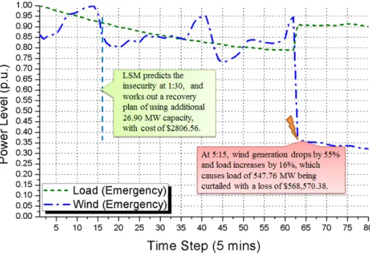
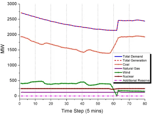
3.4.3 5889-Bus System . . . 48
3.5 Summary . . . 51
4. SPATIO-TEMPORAL WIND FORECASTS . . . 53
4.1 Background . . . 53
4.1.1 Wind Data Source in West Texas . . . 55
4.1.2 Space-time Statistical Forecasting Models . . . 56
4.2 Forecasting Results and Comparison . . . 63
4.3 Scheduling Models for Critical Assessment . . . 65
4.3.1 Day-ahead Reliability Unit Commitment . . . 65
4.3.2 Robust Look-ahead Economic Dispatch . . . 68
4.4 Numerical Examples with Spatio-temporal Forecasts . . . 71
4.4.1 Results and Analysis . . . 71
4.5 Summary . . . 74
5. STOCHASTIC LOOK-AHEAD SCHEDULING . . . 75
5.1 Stochastic Look-ahead Dispatch . . . 77
5.1.1 Near-Real-Time Operation . . . 77
5.1.2 Framework of Stochastic Look-ahead Dispatch . . . 78
5.1.3 Mathematical Formulation . . . 79
5.2 Benefits Illustration for LAED-S . . . 81
5.2.1 Economic Benefits for Stochastic Look-ahead Dispatch . . . . 81
5.2.2 Security Benefits for Stochastic Look-ahead Dispatch . . . 83
5.3 Power System Uncertainty Response . . . 86
5.3.1 Analytical Criterion for Stochastic Dispatch . . . 87
5.3.2 Horizon Division . . . 91
5.4 Scenario Generation . . . 92
5.5 Hybrid Computation Framework . . . 96
5.5.1 Progressive Hedging Algorithm . . . 98
5.5.2 L-shaped method . . . 102
5.6 Innovative Scale Reduction . . . 105
5.7 Numerical Examples with Stochastic Look-ahead Dispatch . . . 113
5.8 Summary . . . 118
6. CONCLUSIONS AND DIRECTIONS FOR FUTURE RESEARCH . . . . 120
6.1 Dissertation Summary . . . 120
6.2 Future Research . . . 122
6.2.1 Trade-offs between Security Enhancement and Computation Burden . . . 122
6.2.2 Security Management under Forecast or Contingency Uncer-tainties . . . 122
6.2.3 Theoretical Study in Pricing under Stochastic Near-real-time Market . . . 123
6.2.4 Probability Methods based Power System Infrastructure Plan-ning . . . 123 REFERENCES . . . 125
LIST OF FIGURES
FIGURE Page
1.1 Renewable portfolio standard policies . . . 1
1.2 Wind power global capacity, 1996-2012 . . . 2
2.1 Information exchange for centralized look-ahead dispatch . . . 13
2.2 Illustrative example for economic performance improvement . . . 17
2.3 The operating uncertainty trend in a look-ahead horizon . . . 19
2.4 Total operating cost over different look-ahead horizon . . . 20
2.5 Total operating cost of high wind forecast uncertainty . . . 21
3.1 Illustrative example of look-ahead SCED feasibility improvement . . . 23
3.2 Power system security management diagram . . . 27
3.3 Illustrative diagram of short-term dispatchable capacity . . . 28
3.4 Conceptual illustration of relaxing variables . . . 33
3.5 Enumeration tree approach to the identification of multiple factors . . 37
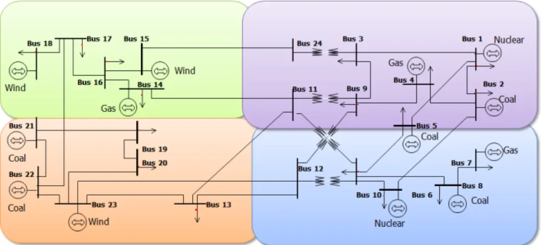
3.6 IEEE RTS-24 system (modified) . . . 42
3.7 The contingency scenario for infeasibility study . . . 44
3.8 Operation of different types of generation (static SCED) . . . 45
3.9 Operation of different types of generation (look-ahead SCED) . . . . 46
3.10 Relaxing variables to energy balancing constraints . . . 47
3.11 Relaxing variables to ramping constraints . . . 48
3.12 Required capacity over look-ahead horizons . . . 49
3.13 Recovery cost over look-ahead horizons . . . 50
4.1 Map of the four locations in West Texas . . . 56
4.2 Wind roses of the four locations in West Texas . . . 57
4.3 Wind speed density at ROAR 2008-2009 . . . 59
4.4 Functional boxplot of daily wind speed at ROAR 2008-2009 . . . 60
4.5 The pressure gradient, Coriolis, and friction forces influence the move-ment of air parcels. Geostrophic wind (left) and real wind (right) . . 62
4.6 Two-layer dispatch model . . . 66
4.7 Distribution of forecast errors under different forecast models . . . 71
4.8 Total operating cost using different forecast models . . . 72
4.9 Operating cost reduction using different forecast models . . . 73
5.1 Wind power forecast accuracy versus forecast horizon . . . 76
5.2 The horizon division of a stochastic look-ahead dispatch . . . 78
5.3 The general flowchart of a stochastic look-ahead dispatch . . . 79
5.4 Illustrative example of economic benefits for a stochastic look-ahead dispatch . . . 81
5.5 Illustrative example of security benefits for a stochastic look-ahead dispatch . . . 84
5.6 Typical uncertainty response to net load uncertainties in a power system 88 5.7 Typical uncertainty response to net load uncertainties over look-ahead horizon . . . 89
5.8 Multi-time-scale uncertainty response under a deterministic look-ahead dispatch . . . 91
5.9 Wind production potential (per unit) under 1000 scenarios generated by Monte Carlo simulation . . . 93
5.10 Wind production potential (per unit) under 1000 scenarios with per-sistence factor PF = 0.7 . . . 94
5.11 Wind production potential (per unit) under 50 representative scenar-ios after scenario reduction process . . . 96
5.13 Decision variables statistics in a yearly and monthly window . . . 106 5.14 Constraints statistics in a yearly and monthly window . . . 107 5.15 Probability assessment for variable fixing and constraints relaxation . 109 5.16 Economic risks for ten consecutive days in July . . . 114 5.17 Percentages of time intervals when stochastic look-ahead dispatch is
needed. . . 115 5.18 Cost savings as the net load uncertainty increases: deterministic
ap-proach versus stochastic apap-proach . . . 117 5.19 Computation time for different economic approaches . . . 118
LIST OF TABLES
TABLE Page
2.1 Illustrative Example: Static Dispatch . . . 17
2.2 Illustrative Example: Look-ahead Dispatch . . . 18
2.3 Overall System Operating Cost under Forecast Uncertainty . . . 21
3.1 Static Dispatch (Infeasible) . . . 24
3.2 Look-ahead Dispatch (Feasible) . . . 24
3.3 Generation Resources Parameters . . . 43
3.4 Corrective Measures under Contingency . . . 43
4.1 Site Information . . . 55
4.2 MAE Values of Different Forecast Models . . . 64
5.1 Scenario Definition for Illustrative Example 1 (Unit: MW) . . . 82
5.2 Dispatch Decisions for Time Interval 1 :Illustrative Example 1 (Unit: MW) . . . 82
5.3 Dispatch Decisions for Time Interval 2: Illustrative Example 1 (Unit: MW) . . . 84
5.4 Scenario Definition for Illustrative Example 2 (Unit: MW) . . . 85
5.5 Dispatch Decisions for Time Interval 1: Illustrative Example 2 (Unit: MW) . . . 85
5.6 Dispatch Decisions for Time Interval 2: Illustrative Example 2 (Unit: MW) . . . 86
5.7 Computation Environment for Numerical Experiments . . . 113
5.8 Average Economic Performance for Stochastic Intervals (per Interval) 114 5.9 Daily Average Economic Performance (post Realization) for Different Types of Dispatch . . . 116
1. INTRODUCTION
1.1 Motivation and Overview
As efforts of reducing the reliance on conventional fossil fuel and mitigating the greenhouse gas emissions, many regions have set ambitious goals of achieving high penetration of renewable energy in the near future (as shown in Figure 1.1)[1, 2]. By the end of 2012, the global installed wind capacity has already reached the level of 283 GW (Figure 1.2) [3]. Intermittent resources such as wind and solar consist a large portion ( up to 83% of the overall renewable capacity). The uncertainties and variability of these resources pose significant challenges to electric power system operations.
Figure 1.1: Renewable portfolio standard policies
as economic dispatch) algorithms with enhanced capability to manage the security risks due to the high variation and uncertainty introduced by intermittent resources and contingencies in electric power systems. In recent years, as an alternative to con-ventional static security constrained economic dispatch (SCED), look-ahead SCED has become a new industry standard in real-time energy market operations [4, 5]. In contrast with the single-stage optimization of static SCED, look-ahead SCED works out a scheduling plan for a future period (e.g., the next 2 hours). By (i) utilizing the accurate most recently updated load and intermittent generation forecasts (e.g., 10-minute ahead forecast) and (ii) incorporating the inter-temporal constraints (e.g., ramp rate), look-ahead SCED exhibits an improved economic performance over static SCED [6].
1.2 Literature Review
The concept of the look-ahead (dynamic) dispatch originated in the 1980s. Ross et. al. proposed a dynamic economic dispatch algorithm for generation units [7]. Carpentier et. al. discuss the coupling between short-term scheduling and dispatch-ing [8]. Raithel et. al. study the improved allocation of generation through dynamic economic dispatch [9]. The major motivation behind conducting look-ahead (dy-namic) economic dispatch was to incorporate the near-term variable load forecast and schedule the system resources cost-effectively. Recent work extends and justi-fies the joint benefits when taking into account the environmental impacts (emission costs, primarily), intermittent resources, and responsive demand resources. Xie et. al. use model predictive control based economic dispatch to co-optimize the eco-nomic and environmental concerns [10]. Later, they generalize the look-ahead model to integrate the price-responsive demand [11] and propose a novel look-ahead in-teractive dispatch internalizing inter-temporal constraints at the distributed energy resources level [12, 13]. Most of these research are focusing on the economic benefits of look-ahead dispatch, the potential added value of look-ahead dispatch in system security enhancement has not been well studied. This research aims at bridging this gap.
In supporting advanced look-ahead dynamic scheduling, accurate forecast method of renewable resources is essential. Therefore, many active efforts are devoted to this area [14]. One of the popular approaches are numerical weather prediction (NWP) approach which produces forecasts based on physical conditions such as terrain, ob-stacle, pressure, and temperature. Landberg proposes an NWP model from which the predictions are generated from the high-resolution limited area model (HIRLAM) of the Danish Meteorological Institute [15]. Negnevitsky et. al. suggest, with accurate
Digital Elevation Models (DEMs) and Model Output Statistics (MOS), specifically tuned NWP models performs well but are still unsuitable for short-term forecast [16]. Whereas NWP models play the key role in day-ahead to several hour-ahead wind forecasting, the computational burden and forecasting accuracy of NWP are still challenging in near-term forecasts (minutes-ahead to hour-ahead). As an alter-native, data-driven statistical wind forecasting has gained increasing attention for near-term forecasts. Extensive research has been devoted to wind power forecasting problems [17, 18, 19, 20]. In short-term wind speed forecasting, statistical models that incorporate spatial information are the most competitive methods [20, 21]. A regime-switching space-time model [22] improves forecasts by 29% and 13% com-pared with persistence forecasts and autoregressive in terms of root mean squared error (RMSE). It is generalized by the TDD model [23] by treating wind direc-tion as a circular variable and including it in the model. Regime-switching models based on wind direction and conditional parametric models with regime-switching substantially reduce variance in the forecast errors [24]. Adaptive Markov-switching autoregressive models [25] are developed for offshore wind power forecasting prob-lems in which the regime sequence is not directly observable but follows a first-order Markov chain. For wind speed forecasting problems, more realistic metrics that have penalization on underestimates and forecasts for small true values are desired for model evaluation [20] instead of RMSE and mean absolute errors (MAE). Power curve error [23] is proposed as a loss function, which links prediction of wind speed to wind power by a power curve and evaluates the loss based on the wind power with penalty on underestimates. This research conducts critical assessment over different statistical forecast models and evaluates the benefits for power system operations.
In the domain of applying advanced optimization algorithms for power system scheduling, many valuable research efforts are devoted to handling the operational
uncertainty concerns. For example, Wang et. al. present a stochastic security-constrained unit commitment (SCUC) algorithm solved by Benders decomposition [26]. Meibom et. al. present a stochastic mixed integer scheduling model where the schedules are updated in a rolling manner as more up-to-date information become available [27]. Ruiz et. al. compare stochastic programming with existing reserve methods and evaluate the benefits of a combined approach for the efficient man-agement of uncertainty in the unit commitment problem [28]. Papavasiliou et. al. justify that a stochastic programming unit commitment policy outperforms conven-tional reserve rules [29]. Hedman et. al. employ statistical clustering techniques to determine the reserve zones based on the power transfer distribution factors (PTD-F) and electrical distances (ED) for uncertainty management [30]. Bertsimas et. al. propose a two-stage adaptive robust unit commitment model in the presence of nodal net injection uncertainty [31]. Wang et. al. formulates a chance-constrained two-stage (CCTS) stochastic unit commitment problem with uncertain wind power output [32]. Ryan et. al. propose a stochastic unit commitment algorithm focusing on the development of a decomposition scheme based on the progressive hedging al-gorithm [33]. Guan et. al. introduce an innovative min-max regret unit commitment model to minimize the maximum regret of the day-ahead decision from the actual re-alization of the uncertain real-time wind power generation [34]. Luh et. al. integrate the discrete Markov process based aggregated wind generation model into stochastic unit commitment problems [35]. This research leverages the advantages of the pro-gressive hedging algorithm and L-shaped method to develop a parallel computation based stochastic look-ahead dispatch.
1.3 Major Contributions
The contributions of this research are from two-fold: electric power engineering and system sciences. The contributions with respect to electric power engineering are suggested as follow:
• Improved economic efficiency in scheduling large scale renewables.
• Early detection and optimal corrective measures for potential insecurities of power systems.
• Improved forecast of renewables via spatio-temporal statistics.
• Efficient stochastic look-ahead dispatch to handle uncertainties in power grid. The contributions with respect to system sciences are suggested as follow: • Enhanced dynamic programming for resource allocation in a temporally and
spatially coupled complex system.
• Early detection and identification of potential infeasibilities.
• Improve resource prediction by leveraging spatial and temporal correlations over large data sets.
• Parallelizable stochastic programming algorithm to optimize systems under uncertainty.
1.4 Dissertation Outline The rest of this dissertation is organized as follows.
Chapter 2 presents the look-ahead dynamic economic dispatch. The model of look-ahead economic dispatch is formulated. Market pricing in look-ahead dispatch
framework is discussed. Illustrative example of a simple system is provided to show the economic benefits of look-ahead dispatch. On the other hand, the impacts of uncertainties on look-ahead dispatch is discussed. Look-ahead dispatch suffers from the high uncertainty in net load. Numerical examples of a modified 24 bus system are conducted to justify the advantages of look-ahead dispatch.
Chapter 3 addresses the security management under a look-ahead dispatch frame-work. The mathematical model of security enhanced look-ahead economic dispatch is formulated. The concept of relaxing variables are introduced. The early detection and optimal corrective measures are presented. Numerical experiments of a modified 24 bus system as well as a 5889 bus practical system are conducted to justify the security benefits of a look-ahead dispatch framework.
Chapter 4 deals with the application of spatio-temporal wind forecast models. An overview of statistical wind forecast models are provided, followed by the introduction of the proposed spatio-temporal wind forecast models. We compare the performance of spatio-temporal wind forecasts using realistic wind farm data obtained from West Texas. For the critical assessment of the forecast models, a day-ahead reliability unit commitment model and a robust look-ahead economic dispatch formulation are pre-sented. Numerical experiments are conducted to verify the benefits of incorporating spatio-temporal wind forecasts.
Chapter 5 explores the benefits and feasibility in applying a stochastic look-ahead economic dispatch algorithm for power system near-real-time operation. Based on the economic risk index, we propose an analytical criterion judging whether a s-tochastic approach is applicable to each dispatch interval. A ss-tochastic look-ahead economic dispatch for near-real-time power system operation is formulated. A hori-zon division technique is applied to divide a look-ahead dispatch horihori-zon into a deterministic portion and a stochastic portion. In order to implement an efficient
stochastic look-ahead dispatch for real-time operation, an innovative hybrid comput-ing architecture is proposed which leverages the progressive hedgcomput-ing algorithm and L-shaped method. By advanced approach to reducing the problem size significantly, the algorithm can operate in a much efficient manner. Numerical experiments of a practical 5889 bus system are conducted to illustrate the effectiveness of the proposed approach.
Chapter 6 summarizes the conclusions of the research and discusses the directions of work that we wish to pursue in the future.
2. LOOK-AHEAD DYNAMIC ECONOMIC DISPATCH∗
This chapter presents the look-ahead dynamic economic dispatch. Look-ahead dynamic economic dispatch is motivated by the need for better algorithms to man-age the operation uncertainty and variability due to high penetration of variable renewable resources (e.g. wind and solar). With the fast development in renewable capacities, variable resources consist a large portion ( up to 83% of the overall renew-able capacity). The uncertainties and variability of these resources pose significant challenges to electric power system operations.
Recently, look-ahead dispatch has been proposed and studied as a mechanism to manage the increasing level of inter-temporal variation in electric energy supply port-folio [7, 36, 37, 38]. Several major Independent System Operators (ISO)/ Regional Transmission Organizations (RTO) are investigating and implementing various ver-sions of look-ahead dispatch [5, 39, 4]. However, new issues arise in implementing look-ahead dispatch.
One issue of implementing look-ahead dispatch is the uncertainty in the forecast of renewable resources and system demand. Many studies are devoted to uncertainty handling in economic dispatch problems. In [40], a probabilistic method is applied to unit commitment in spinning reserve assessment. King, et al. use both deterministic and stochastic approaches to conduct dispatch [41]. Reliability index is introduced to test uncertainty under different formulations. Bouffard, et al. introduce a stochastic security framework into the market-clearing formulation and demonstrate its
advan-∗This section is in part a reprint of the material in the papers: Y. Gu and L. Xie, “Look-ahead
Dispatch with Forecast Uncertainty and Infeasibility Management,” inPower and Energy Society General Meeting, IEEE, San Diego, 2012. Y. Gu and L. Xie, “Early Detection and Optimal Correc-tive Measures of Power System Insecurity in Enhanced Look-Ahead Dispatch,”IEEE Transactions on Power Systems, vol. 28, pp. 1297-1307, 2013.
tage in higher penetration of wind power compared with worst-case deterministic approach [42].
The main objective of this chapter is introduce and justify the benefits of a look-ahead dispatch.
2.1 Look-ahead Security Constrained Economic Dispatch
Security constrained economic dispatch (SCED) is to maximize the total social welfare in power system operating when considering the operating security con-straints such as generators capability limits, ramping limits, and transmission line capacity constraints.
Conventional SCED is conducted only one snapshot every 5 to 15 minutes [43]. Inter-temporal constraints such as generators’ ramping constraints are incorporated by only considering the current generation outputs, which is not designed to handle the future variability of the variable resources.
Furthermore, in conventional static SCED, energy storage dynamic constraints can only be approximately represented in the capacity of charging and discharging for the immediate next time step. Without explicitly considering the inter-temporal energy dynamic constraints, the contribution of the energy system will be very lim-ited.
The look-ahead dispatch is to expand single snapshot-based SCED problem into a multi-stage problem. The temporal constraints (constraints terms) and inter-temporal benefits (objective terms) can be well taken in the optimization, which can improve the feasibility and optimality of the system.
2.1.1 Mathematical Formulation
The mathematical model of the look-ahead dispatch is presented in (2.1) to (2.8).
max :f = T X k=k0 X i∈D Bi(PDik )− T X k=k0 X i∈G CGi(PGik ) + X i∈S EiTλˆTi (2.1)
The objective function (2.1) is to maximize the total social welfare (total customer benefits minus system operating costs). In (2.1), G is the set of generators;D is the set of loads; S is the set of energy storage resources; CGi(PGik is the generation cost of generatori;Bi(PDik ) is the benefit function of loadi; ˆλTi is the unit value of stored energy, which is used to evaluate the energy value of storage resources at the final step in a look-ahead plan P
EiTλˆTi ;
This optimization is subject to various security constraints. X
i∈G
PGik =X i∈D
PDik , k =k0, . . . , T (2.2)
The energy balancing equation (2.2) requires the steady state total supply equal to total demand from time to time, where Pk
Gi is the output level of generatori at time step k;
Eik−1−Eik=4t·PGik , i∈S, k=k0, . . . , T (2.3)
Energy dynamics of storage resources are given by (2.3), which characterize the relationship between the charging/discharging power and the energy level of the resources. Eik is the energy level of energy storage iat time step k.
−Fmax 6Fk 6Fmax, k=k0, . . . , T (2.4)
The branch power flow constraints are provided by (2.4), which can be imple-mented by two inequality constraints. Fk is the vector of branch flow at the time step k and Fmax is the vector of transmission constraints of branches.
−PR i 6∆T(P k Gi−P k−1 Gi )6P R i , i∈G, k =k0, . . . , T (2.5)
The ramping rate constraints of generators are described by (2.5), where PiR is the ramping rate limit of generator i.
Eimin 6Eik6Eimax, k=k0, . . . , T (2.6)
In (2.6), the upper/lower bounds of energy level for storage resources are giv-en, where Emax
i and Eimin are the maximum and minimum energy capacity of the resources.
PGimin 6PGik 6PGimax, k=k0, . . . , T (2.7)
In (2.7), the upper/lower bounds of the power levels of generators are provid-ed, where Pmax
Gi and PGimin are the maximum and minimum power capacity of the resources.
PDimin 6PDik 6PDimax, k =k0, . . . , T (2.8)
The upper and lower bounds of demand are described in (2.8).
2.1.2 Pricing in Look-ahead Dispatch Framework
In deregulated electricity market, the look-ahead dispatch could be implemented in two separate ways: 1) centralized ahead dispatch and 2) decentralized look-ahead dispatch [6]. In the decentralized look-look-ahead dispatch, optimization of multi-time scale horizons takes place at each market participant level (i.e. power plants and demands) and the optimization at system operator level is static [44].
Figure 2.1: Information exchange for centralized look-ahead dispatch
The information exchanging in a centralized look-ahead dispatch is shown in Fig. 2.1. For each time step, market participants (i.e. power plants and demands) submit their offer / bidding curves for the future look-ahead period. The system
operator (ISO/RTO) collects those offer/ bidding curves and runs the look-ahead dispatch to clear the market. The price signals of the look-ahead period will be published. Only the dispatch results of the first step are executed.
In this section, clearing price λ∗ in look-ahead framework is discussed. The relationships between the clearing price λ∗ and various shadow prices are analyzed.
The locational marginal price (LMP) under static economic dispatch has been discussed in [45], which consists of incremental system costs due to incremental demand at the slack bus, incremental network losses, and transmission congestion terms.
We propose the definition of LMP in look-ahead SCED framework as the incre-mental generation cost over the entire look-ahead horizon due to increincre-mental demand increase at bus i in the interval k.
LM Pik= ∂f ∂Pk
Di
(2.9)
The Lagrange function of the look-ahead SCED formulation from (2.1) to (2.8) can be written as
L=f +X k λkel(X i∈G PGi− X i∈D PDi) +X k X i∈S λkEi(Eik−1−Eik−PGik ) +X k X i∈G µkRUi(PGik+1−PGik −PGiRU) +X k X i∈G µkRDi(PGik+1−PGik −PGiRD) +X k X i∈G µkGUi(PGik −PGimax) +X k X i∈G µkGDi(PGik −PGimin) +X k X i∈L µkCUi(Fik−Fimax) +X k X i∈L µkCDi(Fik−Fimin) +X k X i∈S µkEUi(Eik−Eimax) +X k X i∈S µkEDi(Eik−Eimin) (2.10) In (2.10),λk
el is the dual variable of energy balance equation at interval k, λkEi is the dual variable of energy dynamic equation of storage i, at interval k, µk
RUi and µk
RDi are the dual variables of ramping constraints of generator i at interval k, µkGUi and µk
GDi are the dual variables of capacity constraints of generator i at interval k, µk
CUi and µkCDi are the dual variables of transmission constraints of line i at interval k, µkEUi and µkEDi are the dual variables of energy upper and lower bound of storage i at interval k.
gradients of L should equal to zeros, and thus yield (2.11) and (2.12). ∂L ∂PD = ∂f ∂PD −λel−µTC ·H (2.11) ∂L ∂PG = ∂f ∂PG +λel+µR+µG+µTC ·H (2.12)
Where, PD is the vector of PDik , PG is the vector of PGik , λel is the vector of λkel, µC is the vector of the sum ofµkCUi andµCDik ,µRis the vector of the sum ofµkRUi and µk
RDi, andµG is the vector of the sum ofµkGUi and µkGDi. H is the distribution factor matrix which characterizes the power flow in each branch when additional MWh of energy is transmitted from the corresponding bus to the slack bus.
(2.11) can be rearranged into (2.13) which is exactly the LMP in look-ahead SCED , consistent with the definition in (2.9).
∂f ∂PD
=λel+µTC ·H (2.13)
Therefore, the LMP in look-ahead SCED framework at interval k can be calcu-lated by the dual variable of energy balance equations and transmission constraints as well as the distribution factor matrix at interval k.
(2.12) indicates the relationship between theλelwhich is the price at slack bus and other dual variables including the ones corresponding to the inter-temporal ramping constraints.
Therefore, the inter-temporal ramping constraints will have impact on the LMP but this ramping component is naturally embedded into λel the dual variable of energy balance equation. The LMP in look-ahead SCED can be calculated by (2.13).
2.1.3 Advantages of Look-ahead Dispatch
In this subsection, we use simple system to illustrate the economic advantages of look-ahead dispatch.
Figure 2.2: Illustrative example for economic performance improvement
Table 2.1: Illustrative Example: Static Dispatch 0:00 0:05 Available Wind 65MW 80MW G1 65MW 60MW G2 40MW 25MW G3 5MW 5MW Load 110MW 90MW
The illustrative system is shown in Fig. 2.2. There are three generators the param-eters of which are indicated. We apply both static dispatch and look-ahead dispatch to perform the scheduling for the system. The scheduling results are presented in Tab. 2.1 and Tab. 2.2. As we can see, the total generation cost in look-ahead dispatch ($198.75) is 12.5% lower than in static dispatch ($227.08). The static dispatch will
Table 2.2: Illustrative Example: Look-ahead Dispatch 0:00 0:05 Available Wind 65MW 80MW G1 65MW 80MW G2 20MW 5MW G3 25MW 5MW Load 110MW 90MW
optimize every step separately. The lower marginal cost of coal generation enables its high output in the first step. However, due to the ramping rate limits, the higher output of coal power plant in the first step limits the reduction of coal generation in the second step and thus the more inexpensive wind generation cannot go up to 80MW but gets curtailed by 20 MW. The look-ahead dispatch will optimize the two steps together. In order to well-utilize wind generation, the expensive but fast ramp natural gas unit is scheduled at higher level in the first step, which enables fully utilization of wind generation at the second step. Therefore, the overall generation cost is lower than the cost in static dispatch.
2.2 Impacts of Uncertainties
Without presence of uncertainty, look-ahead SCED can produce more cost-effective dispatch results than static dispatch can. However, the look-ahead approach may suffer from uncertainties such as wind/solar forecast errors, load forecast errors, un-expected unit outages, etc. Under high level of uncertainty, the dispatch solutions of longer horizon look-ahead decision-making may not be as good as the ones of shorter horizon look-ahead dispatch.
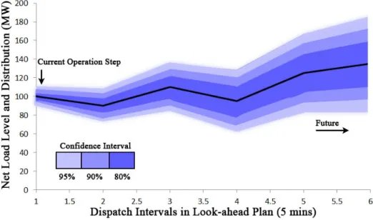
It is illustrated in Fig. 2.3 that as the horizon goes longer, the operating uncer-tainty in future steps increases.
Figure 2.3: The operating uncertainty trend in a look-ahead horizon
2.3 Numerical Examples with Look-ahead Dispatch
In this section, we presented the numerical examples to illustrate the look-ahead dispatch. System setup details are provided in [46].
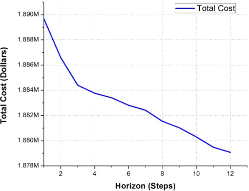
The total system operating cost of one day for different look-ahead horizon is presented in Fig. 2.4. The case with look-ahead horizon of one step is the static economic dispatch. It can be observed that in the look-ahead economic dispatch, the system operating cost could be reduced compared with using conventional static economic dispatch. With perfect system knowledge (no prediction errors), longer look-ahead horizon could lead to lower operating cost.
However, as discussed in Section 2.2, the performance of look-ahead dispatch may suffer from the uncertainties in future steps such as wind forecast errors. Given the high wind forecast errors (30% of actual value with increasing pattern), it can be observed in Fig. 2.5 that the longer look-ahead horizon may even lead to a poorer
Figure 2.4: Total operating cost over different look-ahead horizon
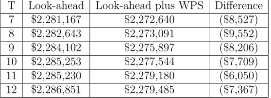
performance in economic dispatch compared with the short look-ahead horizon. This is because the wind forecast errors in the long run are greater than the ones in the short run. The introduction of those errors could undermine the optimality of the solution. With the weighted predictive scheduling (WPS), as is shown in Tab. 2.3, the negative impacts from future uncertainties can be reduced and mitigated so the system operating cost can be lower than the one without WPS.
Therefore, as we discussed in this Chapter, look-ahead dispatch has economic advantages over the conventional static dispatch. However, under high uncertainty level, a look-ahead dispatch solution with longer horizon may suffers from the low quality of forecast and performs not as good as a solution with shorter horizon.
Table 2.3: Overall System Operating Cost under Forecast Uncertainty T Look-ahead Look-ahead plus WPS Difference
7 $2,281,167 $2,272,640 ($8,527) 8 $2,282,643 $2,273,091 ($9,552) 9 $2,284,102 $2,275,897 ($8,206) 10 $2,285,253 $2,277,544 ($7,709) 11 $2,285,230 $2,279,180 ($6,050) 12 $2,286,851 $2,279,485 ($7,367)
3. EARLY DETECTION AND OPTIMAL CORRECTIVE MEASURES∗
In Chapter 2, the economic benefits of look-ahead dispatch has been presented. This chapter discusses the security benefits of look-ahead dispatch. As the economic benefits have been well studied in academia and widely accepted in industry [7, 8, 9, 44], the potential added value of look-ahead dispatch in system security enhancement has not been well investigated. This research aims at bridging this gap.
3.1 Power System Security
Power system security refers to the capability of a system to withstand sudden disturbances or an unexpected loss of components [47]. In conventional power system operations, due to the limited time framework allowed for analyzing and responding to security problems, maintaining system security in real-time is a significant chal-lenge [48]. Violations of system security constraints due to high variability in both demand and generation can cause severe consequences in real-time operations [49]. By taking advantage of the look-ahead SCED framework, the proposed look-ahead security management (LSM) can, at an earlier stage, detect and identify the violated security constraints which can cause potential security problems to the system. The violation of the constraints can furthermore be quantified. In addition, an optimal corrective plan can be worked out with minimal recovery costs for the system.† With LSM in the look-ahead SCED framework, it is possible to reduce the impacts of an
∗This section is in part a reprint of the material in the papers: Y. Gu and L. Xie, “Look-ahead
Dispatch with Forecast Uncertainty and Infeasibility Management,” inPower and Energy Society General Meeting, IEEE, San Diego, 2012. Y. Gu and L. Xie, “Early Detection and Optimal Correc-tive Measures of Power System Insecurity in Enhanced Look-Ahead Dispatch,”IEEE Transactions on Power Systems, vol. 28, pp. 1297-1307, 2013.
†Recovery cost is the cost of the deployed corrective measures to recover the system from
emergency ramp event‡ (e.g., Feb. 26th, 2008 in the Electric Reliability Council of Texas (ERCOT)§) and enable a more robust and cost-effective system operation.
3.2 Security Enhanced Look-ahead Dispatch
Different from conventional static dispatch, look-ahead SCED expands the one-snapshot SCED into a multi-one-snapshot SCED. Inter-temporal constraints (constraint terms) and inter-temporal benefits (objective terms) can then be implemented in the optimization, which improves not only the optimality but also the feasibility of the dispatch problem.
3.2.1 Security Advantages: An Illustrative Example
In this section, illustrative example is used to demonstrate that besides the im-provement in the economic benefits, another major advantage of look-ahead SCED is the improvement in feasibility to the dispatch problem, as shown in Fig. 3.1.
Figure 3.1: Illustrative example of look-ahead SCED feasibility improvement
There are two power sources in the illustrative example: a wind farm with 40 MW capacity and a coal power plant with 80 MW capacity and a 10 MW/15 mins ramping
‡A ramp event refers to the situation in which demands or intermittent generations (e.g., wind)
increase/decrease in a short-term period, which poses difficulty for the system to balance the demand with the available generation resources.
§On Feb. 26, 2008, the wind generation dropped by about 1400 MW over ten minutes, while
the demand increased by 4412 MW at the same time due to the weather conditions, which caused ERCOT to cut the demand by 1100 MW [50].
capability. In the illustrative example, both static SCED and look-ahead SCED are applied to the same scenario, as shown in Table 3.1 and Table 3.2, respectively.
Table 3.1: Static Dispatch (Infeasible) 0:00 0:05 Available Wind 35MW 25MW G1 60MW 70MW G2 35MW 25MW Total Generation 95MW 95MW Load 95MW 105MW
With static dispatch, when the wind generation drops from 35 MW to 25 MW and demand increases from 95 MW to 105 MW, the coal power plant cannot ramp up in such a short period and therefore a loss of load of 10 MW occurs.
Table 3.2: Look-ahead Dispatch (Feasible) 0:00 0:05 Available Wind 35MW 25MW G1 70MW 80MW G2 25MW 25MW Total Generation 95MW 105MW Load 95MW 105MW
With look-ahead SCED, this problem can be avoided. The change in wind re-sources and demand will be considered beforehand; although more coal capacity is used instead of inexpensive wind generation in the first interval, the demand can be satisfied by the total generation in the second interval. This example illustrates that,
due to the fact that multi-stage is considered within look-ahead SCED, the feasibil-ity of the dispatch problem with look-ahead SCED improves upon the conventional dispatch approach.
3.2.2 Formulation of the Enhanced Look-ahead Dispatch
Extended from the model presented in Section 2, the security enhanced look-ahead SCED model presented in this paper incorporates contingency security con-straints with the introduction of short-term dispatchable capacity (STDC).
The security enhanced look-ahead SCED is formulated as (3.1)-(3.11):
min :f = T X k=1 X i∈G CGi(PGik ) (3.1) Subject to X i∈Gj PGik −PDjk =PNjk (θ), k= 1. . . T, j ∈N (3.2) X i∈G PSUik >SUDk, k= 1. . . T (3.3) X i∈G PSDik >SDDk, k= 1. . . T (3.4) −Fmax 6Fk 6Fmax, k= 1. . . T (3.5) −PR Di 6 1 ∆T(P k Gi−Pk −1 Gi )6P R U i, i∈G, k= 1. . . T (3.6) PGik +PSUik 6PGimax, i∈G, k= 1. . . T (3.7) PGik −PSDik >PGimin, i∈G, k= 1. . . T (3.8) PGimin 6PGik 6PGimax, k= 1. . . T (3.9) 06PSUik 6PU iR∆T, k= 1. . . T (3.10) 06PSDik 6PDiD∆T, k= 1. . . T (3.11)
where, G is the set of all available generators; Gj is the set of generators in bus j, CGi(PGi)k is the marginal generation cost of generator i; PGik is the output level of generator i at time step k, with Pmax
Gi and PGimin as its upper and lower bounds; PDik is the load level of bus i at time step k; Pk
Nj(θ) is the nodal power injection in bus j at time step k, Pk
SUi and PSDik are the proposed short-term dispatchable capacity (STDC) of generator i at time step k; Fk is the vector of the branch flow at time step k and Fmax is the vector of the branches’ capacity.
The objective function (3.1) is to minimize the total generation cost. Equality constraints (3.2) are the nodal energy balancing equations. Inequality constraints (3.3) and (3.4) are the constraints of upward/downward STDC requirement con-straints. The inequality constraints from (3.5) to (3.11) are transmission capacity constraints, ramping capability constraints, mixed generator capacity constraints, and the upper and lower bounds of the decision variables.
By considering network losses, the nodal injectionPNjk (θ) is given by
PNjk (θ) = X j:(i,j)∈E
[0.5Plossk (θi, θj)−bijsin(θi−θj)] (3.12)
where E is the set of branches, θi is the voltage phase angle at bus i, and bij is the susceptance of branch (i, j). The nodal network lossPk
loss(θi, θj) can be approximated by its piecewise linear expression [51]. By using a second-order approximation of sin(·), (3.12) can be formulated as (3.13) subject to constraints (3.14).
PNjk (θ)≈ X j:(i,j)∈E
[0.5gijX l∈L
νijlθlij−bij(θi−θj)] (3.13)
of the lth block of voltage phase angle.
06θlij 64Θ, l= 1. . . L (3.14)
Figure 3.2: Power system security management diagram
Due to the operational uncertainties and potential contingencies in an electric power grid, only satisfying security constraints under current normal condition is not enough to ensure the system security. Therefore, power engineers introduce the concept of the “Alert” state, as shown in Fig. 3.2 [52]. An “Alert” state is defined that all the components of a system are working within their operating limits only under non-contingency scenario. The “Normal” state requires all components functioning well even under assumed contingencies(e.g., N-1). Therefore, in order to operate the system in the “normal” state, extra reserve capacity is required.
In many areas, determination of reserve capacity is within the day-ahead u-nit commitment decision-making layer. We introduce the concept of short-term
dispatchable capacity (STDC) which can handle the uncertainty and variations at the real-time economic dispatch layer. This can provide extra margin for the power system operational security, and work as indicators for inadequacy of spin-ning/nonspinning reserves.
Figure 3.3: Illustrative diagram of short-term dispatchable capacity
The idea of STDC is illustrated in Fig. 3.3. Due to the uncertainty in demand, intermittent resources and the potential contingency of the units, sudden changes may lead to imbalances between the generation and the demand. The rest of the system units (not affected by the contingency) should respond in a short time and compensate for the system imbalances. Every generator has its dispatchable region, which is the distance from the current dispatch point (CDP) to its maximum output level. Due to the ramping constraint of each generator, the actual dispatchable capacity within a short period is generally less than the total capacity. We define the short-term dispatchable capacity (STDC) asthe maximum capacity which can be
dispatched up (down) within one dispatch interval.
As shown in Fig. 3.3, given the ramping constraint, the dispatchable capacity within one dispatch interval is the STDC. The capacity required by minimum output constraint is the non-dispatchable capacity (NC). The capacity which is limited by the ramping constraint and cannot be dispatched within one dispatch interval is the short-term non-dispatchable capacity (STNC). STDC, NC, and STNC compose a complete portfolio of the installed capacity. The cumulative STDC indicates the overall ramping capability of the entire system to cope with variations in net load (demand - generation of intermittent resources) or generation inadequacy caused by a contingency.
We formulate (3.3) and (3.4) as short-term responsive N-1 contingency con-straints. If (3.3) and (3.4) are satisfied, it can guarantee that the power system will have enough ramping capability to cope with the uncertainties and variations given the required confidence interval α (e.g., 95%).
We consider the following contingency events in evaluating the STDC require-ments.
• The system doesn’t have any generators failure while an unexpected change in intermittent resources and demand exceeds the total ramping capability of the system.
• The system has one generator failure, while an unexpected change in intermit-tent resources and demand exceeds the ramping capability of the rest system (unaffected by the contingency).
(3.16), respectively. PSAU = [Y i∈G (1−Pfi)][1−φ( SUD σN L )]+ X i∈G Pfi[ Y j∈G j6=i (1−Pfj)][1−φ( SUD −PGimax σN L )] (3.15) PSAD = [Y i∈G (1−Pfi)][1−φ(−SDD σN L )]+ X i∈G Pfi[Y j∈G j6=i (1−Pfj)][1−φ(−SDD−P max Gi σN L )] (3.16)
In (3.15) and (3.16), PSAU(D) are the probability of short-term dispatchable alert (upward/downward), which indicates whether the system-wide ramping capability is enough for handling the potential contingency scenarios , Pfi is the probability of failure of the unit i, σN L is the variance of net load, andφ(·) is the cumulative dis-tribution function of a standard normal disdis-tribution. Given the confidence interval, the requirement of STDC can be determined by equation solver in the optimization toolbox of Matlab.
By incorporating the short-term responsive contingency constraints into the pro-posed look-ahead security management, it enables look-ahead dispatch predicting and quantifying not only the risks to the current status but also the risks under var-ious potential contingency scenarios. By optimization, the utilization of the short-term dispatchable resources is maximized and the shortage of the ramping capability is minimized and reported to the system operator in advance. The valuable infor-mation provided could be used to check the adequacy of the system reserve or as a reference for further deployment of other resources.
3.3 Algorithm for Early Detection and Corrective Measures
A major advantage of look-ahead economic dispatch is to better utilize available resources to enable a larger feasibility region, as discussed in the previous section. However, due to the uncertainty of the renewable resources and potential contin-gencies, there is always the chance that a feasible dispatch plan which satisfies all security constraints does not exist. We define these situations as infeasibility in look-ahead SCED. The infeasibility is related with insecurity of system operation. It is possible to improve the robustness and security of scheduling operation by handle infeasibility issues appropriately.
For MPC-based optimization problems, there exist techniques to handle infeasi-bility issues. In [53, 54, 55, 56], a feasible MPC problem is recovered from infeasiinfeasi-bility by dropping the violated constraints. Rawlings et al. propose and justify the min-imal time approach, which removes the state constraints in the early stages of the infinite horizon problem to make it feasible [55, 56]. However, these approaches are not able to distinguish the relative importance of the various constraint violations. In power system operations, it is important to consider the priority level of differ-ent constraints. In [54, 57], Adersa et al. propose a method of recovering from infeasibilities that involves a prioritization of the constraints. The lowest prioritized constraints are dropped if the online optimization problem becomes infeasible. How-ever, this method cannot quantify how much the constraint gets violated. Also, directly ignoring the infeasible constraints is sometimes unacceptable in practical power system operations. Another approach to solving infeasible MPC problems in which the constraints have different priorities is proposed by Tyler et al.[58]. In their approach, integer variables are introduced to handle the prioritization in an optimal problem. By solving a sequence of mixed-integer optimization problems, the size of
the violation of the constraints is minimized in terms of the prioritization. In [59], Vada et al. propose a method which utilizes a single-objective linear problem to handle infeasibility.
Starting from the previous work [60, 61] on handling the infeasibility of MPC problems, we propose a look-ahead security management (LSM) technique. With the proposed LSM technique, look-ahead economic dispatch not only improves the system feasibility but also predicts and identifies the infeasibility which may occur in the future. The violation of infeasible constraints, which is of great concern (or interest) to the system operators, can be quantified. Furthermore, the LSM technique can help in developing an optimal solution to recover the system from infeasibility with minimal recovery costs.
3.3.1 Relaxing Variables
Relaxing variables are introduced to handle infeasibilities. They are deployed
to relax the constraints and make the problem feasible. High penalty terms asso-ciated with the relaxing variables are added in the objective function to eliminate the chances that the relaxing variables become alternatives to the original decision variables when the problem is feasible.
Fig. 3.4 illustrates the relaxing variables by distinguishing it with slack variables. A slack variable characterizes the distance from the current operating point to the boundary of the feasible region, which can ensure that the current operating point is within its feasible region. The relaxing variablerat optimality indicates the minimal distance from the current status to the status which gives a feasible solution.
3.3.2 Early Identification of Infeasibility
Infeasibility in economic dispatch is usually related to security problems in the physical power system, which refers to certain violations of the operating constraints
Figure 3.4: Conceptual illustration of relaxing variables
(e.g., the overloading of transmission lines, generators’ ramping constraints and so on) or to regional or system-wide imbalances between the energy supply and demand. Any of these violations may cause contingencies or blackouts in the power system, and lead to severe consequences.
In power system real-time operations, it is very important to identify potential security problems in advance. The available measures for handling security problems depend on how much time remains for taking the measures. If the security issue is detected one to two hours ahead, a much broader set of corrective measures can be deployed. On the other hand, if the security violation is detected only 10-15 minutes prior to real-time, the number of corrective measures available are much fewer.
The proposed approach implemented in a look-ahead scheduling framework en-ables the scheduling framework to identify future security risks.
Relaxing variables can be introduced into security constraints (3.2), (3.5), (3.6), (3.9)-(3.11) and the problem can be formulated as follows:
X i∈Gj PGik −PDjk +rNjk =PNjk (θ), k= 1. . . T, j ∈N (3.17) −Fmax−rk F 6F k 6Fmax+rFk, k= 1. . . T (3.18) −PR i −r k Ri 6 Pk Gi−P k−1 Gi ∆T 6P R i +r k Ri, i∈G (3.19) PGimin−rkGi 6PGik 6PGimax+rkGi, i∈G, k= 1. . . T (3.20) 06PSUik 6PU iR∆T +rkSUi, i∈G, k= 1. . . T (3.21) 06PSDik 6PDiD∆T +rkSDi, i∈G, k= 1. . . T (3.22)
where rkNj are the relaxing variables of the nodal energy balance equations, rkF are the relaxing variables of the transmission constraints, rRik are the relaxing variables of the ramping constraints, rk
Gi are the relaxing variables of the generator capacity constraints, and rk
SUi,rSUik are the relaxing variables of the upward/downward short-term dispatchable capacity constraints, respectively.
By incorporating the relaxing variables, the objective function of the look-ahead SCED can be formulated as (21).
minf = T X k=k0 X i∈G CGi(PGik )
+I(rNjk , rF, rRi, rGi, rSUi, rSDi) (3.23)
I(.) is defined as the identification function of the violated constraints. I(.) is suggested to be modeled as a linear or a quadratic function ¶. The coefficients of
¶IfI(.) is a linear function, the relaxing variables should be non-negative and then the relaxing
variables of bidirectional constraints such as ramping constraints, capacity constraints can be split into two parts which indicate the violations of upward and downward constraints, respectively.
the relaxing variables in I(.) indicate the sensitivity of the detection of constraints from various categories (e.g., ramping, transmission capacity). Because infeasibility may be caused by a violation of multiple constraints, the sensitivity of the different constraints must be specified according to the interest of detection. For example, if the system operator is more concerned with (or more interested in) the violation of the energy balance constraint than of the other constraints, the sensitivitysj, j ∈Ci of the constraints in that category Ci should be higher than the sensitivity of the constraints in the other categories Cl, l6=i.
ηj = max
i (|ξi|)χ sγjj (k)
, sj ∈(0,1), χmax(|ξi|) (3.24)
The coefficients of relaxing variable ηj are given by (3.24). In (3.24), γj(k) is the discrimination degree among the constraints over different time steps. γj(k) is the function of time step k, ξi is the coefficient of the ith decision variable in the original objective function, and χ is the parameter to differentiate the relaxing variable terms from the original decision variable terms. Therefore, χ is suggested to be a large number (e.g., 104).
For a conservative look-ahead strategy, it is preferred to identify the potential risks in an earlier rather than a later stage. The sensitivity of function I(.) subject to constraints at different stages is suggested to be monotonically decreasing as time step k increases. This is implemented by the discrimination degree γj(k), which is a function of time step k in a look-ahead plan, as described in (3.25). In addition, the choice of coefficientςj needs to obey (3.25) in order to guarantee the priority relation-ship of the various constraint categories at all time steps (e.g., ramping constraints versus transmission capacity constraints).
γj(k) = ςj
k + 1,jmin∈Cu(sj) γj(1)
>max
j∈Cv(sj),0< u < v (3.25) The linear form of I(.) is presented in (3.26), where the relaxing variables and the corresponding coefficients are in vector form.
I(r) =ηelTrel+ηETrE +ηFTrF +ηRTrR+ηGTrG (3.26)
In look-ahead SCED real-time operations, if the whole plan is feasible, all the relaxing variables are equal to zero and the optimal solution is the same as for the look-ahead SCED in (3.1). However, if infeasibility exists, the corresponding relaxing variable becomes positive. The value of the relaxing variable indicates how much the violation of that constraint is. With the appropriate configuration of the relaxing variables in (3.26), the solution of the relaxed problem identifies and quantifies the potential insecurity in the system.
Due to the sophistication of power system operations, sometimes infeasibility can be caused by the violation of multiple constraints belonging to different categories (e.g., ramping rates v.s. transmission constraints). It is helpful to identify all of the potential factors causing the security issues and report the information by category in terms of system operators’ prioritized concerns. We propose an enumeration tree approach in the LSM to accomplish this.
The sets of security constraint categoriesCj ={ constraints | belong to security constraint categoryj}are defined in terms of their priority to the operators’ concerns (or interests): Cj has a higher priority to the system operator than Ci, where 0 < j < i. The algorithm doing the enumeration is described as follows.
Figure 3.5: Enumeration tree approach to the identification of multiple factors
Step 1 (Initialization): Generate the initial full constraint setCT =C1SC2S...SCN, configure the coefficients of relaxing variable ηi based on (3.24). Go to Step 2. Step 2 (Optimization): Solve the infeasibility identification problem (3.23) subject
to (3.17)-(3.22). Go to Step 3.
Step 3 (Termination test): If the feasibility region of the relaxed problem is empty, namely Sk = ∅, the identification process is terminated. It is reported that the constraints of the category at the current level of concern k do not cause the infeasibility and any constraints with lower priority{j|j > k}do not cause the infeasibility either. End the program, otherwise go to Step 4.
Step 4 (Extension): If the feasibility region of the relaxed problem is not empty, namely Sk 6=∅, however, all the non-zero relaxing variables do not belong to the category of the current level of concern k. The system operator is to be informed that the constraints of the category at the current level of concern
k do not cause the infeasibility and the infeasibility is caused by some lower prioritized constraints {j|j > k}. Go to Step 6, otherwise, go to Step 5. Step 5 (Selection): The system operator is going to be reported the constraints
with non-zero relaxing variables which are responsible to the infeasibility. Go to Step 6.
Step 6 (Configuration): Set the coefficients of all the constraints which belong to the category of the current level of concern k to zero, namely ηj = 0, j ∈ Ck. Move to the next level k =k+ 1. Go back to Step 2.
The whole process is depicted in Fig 3.5. By means of this process, the system operators are informed of not only the factors about which they care the most but also of all the other potential factors causing this infeasibility, ranked in the order of their prioritized concerns.
3.3.3 Optimal Corrective Solution
With the concept of relaxing variable, the optimal corrective solution can be worked out at a minimal operating cost when system operations are infeasible.
RM ={rMi|available measures for system recovery} (3.27)
There are various corrective measures which can help the system recover from infeasibility (e.g., spinning reserve, non-spinning reserve, responsive demand, the fast-response unit, and tie-line support). Different corrective measures have different response speeds and operating costs. Generally, fast resources are more valuable (and expensive) than slow resources. Each corrective measure can be represented by
a relaxing variable rMi. The set of all the available measures for system recovery is represented by RM in (3.27).
minfR =f +R(rM) (3.28)
The objective function of the optimal corrective solution can be modified from the original objective function (3.1) to the objective function of (3.28). R(r) is the recovery cost function, which can be defined as a linear function of the relaxing variables rM. Sometimes, there might be a non-linear relationship between the cost and capacity of the corrective measures. It is suggested to use a linear step-wise model to formulate this relationship for the sake of algorithm efficiency and simplicity. The coefficients of R(r) are given by the marginal operating cost of the various corrective measures.
g(x) +rM >0, r, rM >0 (3.29)
In the relaxed problem, the security constraints are formulated as (3.29). The original constraints g(x) may be impacted by some corrective measures and thus get relaxed. rM are the relaxing variables of the corrective measures. By solving this problem (3.28) to (3.29), an optimal corrective plan is worked out, which can recover the system from infeasibility at the lowest operating cost.
It should be noted that the mathematical model should be modified according to the practical circumstances of the power system. The introduction of relaxing variables is suggested to take into account the results of the infeasibility identification in terms of the time steps and areas impacted by the infeasibility as well as by the
degree of the violation. According to (3.28) and (3.29), a general formulation for an optimal corrective solution is provided in (3.30) - (3.38).
minfR= T X k=k0 X i∈G CGi(PGik ) +RM(rT IE, rDR, rSR, rN R, rLS) (3.30) X i∈G PGik +rT IEk +rDRk +rkSR+rN Rk +rLSk =X i∈D PDik (3.31) −Fmax 6FRk6Fmax (3.32) −PiR∆T 6PGik −PGik−1 6PiR∆T, i∈G (3.33) PGimin 6PGik 6PGimax (3.34) PGik +PSUik 6PGimax, i∈G, k= 1. . . T (3.35) PGik −PSDik >PGimin, i∈G, k= 1. . . T (3.36) 06PSUik 6PU iR∆T, k= 1. . . T (3.37) 06PSDik 6PDiD∆T, k= 1. . . T (3.38)
The objective function (3.30) is to minimize the total operating cost, which in-cludes the ordinary cost of maintaining energy balancing in the system and the additional cost of corrective measures to recover the system from infeasibility. rT IEk represents the capacity of tie-line support. rDRk represents the amount of responsive demand to be used. rk
SR represents the capacity of spinning reserve to be used. rN Rk represents the capacity of non-spinning reserve to be used. rk
LS, as the last resort, is the amount of load which has to be cut to ensure the system security. The corrective
measures discussed here mainly help to relieve the energy balancing constraint by providing additional capacity or by reducing the demand level (3.31). The addition-al corrective capacity may addition-also affect the branch flow. Therefore, the transmission capacity constraints are updated to (3.32), where the vector of branch flow FRk is calculated by the distribution factor matrix and the nodal injections of both the orig-inal injections and also the additional corrective injections. The corrective measures in this example do not impact the generators’ capacity and ramping constraints. Hence, (3.33) - (3.34) remain the same.
3.4 Numerical Examples with Security Enhanced Look-ahead Dispatch The proposed early detection and optimal corrective measures are tested in a 24-bus system and a practical 5889-24-bus system. Details of the system setup of the 24 bus system are presented in Section 3.4.1, and the results and analysis are provided in Section 3.4.2. The system description and simulation results of the practical system are given in Section 3.4.3. The simulations for the two systems are conducted on a Intel i7-990X 3.47GHz desktop computer with Matlab 2011a, IBM ILOG CPLEX v12.2, and Windows 7 operating system.
3.4.1 Simulation Platform Setup of 24 Bus System
The numerical example is modified from the IEEE Reliability Test System (RTS-24) [62]. The simulation duration is 24 hours with 5 minute intervals. The look-ahead horizon ranges from 5 minutes to 4 hours (4 hours by default). Load and wind profiles for 48 hours are collected from ERCOT [63]. Wind generation forecast errors are introduced with a linearly-increasing pattern from 1% to 15% of the actual wind generation potential. Loads are scaled and factored out according to the portions of the different buses [64].