University of California, Berkeley
U.C. Berkeley Division of Biostatistics Working Paper Series
Year Paper
Collaborative Targeted Maximum Likelihood
Estimation
Mark J. van der Laan
∗Susan Gruber
†∗University of California - Berkeley, [email protected] †UC Berkeley, [email protected]
This working paper is hosted by The Berkeley Electronic Press (bepress) and may not be commer-cially reproduced without the permission of the copyright holder.
http://biostats.bepress.com/ucbbiostat/paper246 Copyright c2009 by the authors.
Collaborative Targeted Maximum Likelihood
Estimation
Mark J. van der Laan and Susan Gruber
Abstract
Collaborative double robust targeted maximum likelihood estimators represent a fundamental further advance over standard targeted maximum likelihood estima-tors of causal inference and variable importance parameters. The targeted maxi-mum likelihood approach involves fluctuating an initial density estimate, (Q), in order to make a bias/variance tradeoff targeted towards a specific parameter in a semi-parametric model. The fluctuation involves estimation of a nuisance param-eter portion of the likelihood, g. TMLE and other double robust estimators have been shown to be consistent and asymptotically normally distributed (CAN) under regularity conditions, when either one of these two factors of the likelihood of the data is correctly specified.
In this article we provide a template for applying collaborative targeted maxi-mum likelihood estimation (C-TMLE) to the estimation of pathwise differentiable parameters in semi-parametric models. The procedure creates a sequence of can-didate targeted maximum likelihood estimators based on an initial estimate for Q coupled with a succession of increasingly non-parametric estimates for g. In a departure from current state of the art nuisance parameter estimation, C-TMLE estimates of g are constructed based on a loss function for the relevant factor Q 0, instead of a loss function for the nuisance parameter itself. Likelihood-based cross-validation is used to select the best estimator among all candidate TMLE estimators in this sequence. A penalized-likelihood loss function for Q 0 is sug-gested when the parameter of interest is borderline-identifiable.
We present theoretical results for “collaborative double robustness,” demonstrat-ing that the collaborative targeted maximum likelihood estimator is CAN when Q and g are both mis-specified, providing that g solves a specified score equation
implied by the difference between the Q and the true Q 0.
This marks an improvement over the current definition of double robustness in the estimating equation literature.
We also establish an asymptotic linearity theorem for the C-DR-TMLE of the tar-get parameter, showing that the C-DR-TMLE is more adaptive to the truth, and, as a consequence, can even be super efficient if the first stage density estimator does an excellent job itself with respect to the target parameter.
This research provides a template for targeted efficient and robust loss-based learning of a particular target feature of the probability distribution of the data within large (infinite dimensional) semi-parametric models, while still providing statistical inference in terms of confidence intervals and p-values. This research also breaks with a taboo (e.g., in the propensity score literature in the field of causal inference) on using the relevant part of likelihood to fine-tune the fitting of the nuisance parameter/censoring mechanism/treatment mechanism.
1
Introduction
Researchers acknowledge that questions about our infinite-dimensional, semi-parametric world are not well-addressed by semi-parametric models. More sophis-ticated tools are needed to wrest meaning from data. We can and should develop and utilize methods specifically designed to estimate a relatively small-dimensional precisely specified parameter within such a semiparametric model that is identifiable from the data. The ideal method would be entirely a pri-ori specified, have desirable statistical properties, avoid reliance on ad hoc or arbitrary specifications, and be computationally feasible.
Suppose one observes a sample of independent and identically distributed observations from a particular data generating distribution P0 in a
semi-parametric model, and that one is concerned with estimation of a particular pathwise differentiable parameter of the data generating distribution. A pa-rameter should be viewed as a mapping from the semiparametric model to the parameter space (e.g., real line). A parameter mapping is pathwise dif-ferentiable at P0 if it is differentiable along all smooth parametric sub-models
through P0, and its derivative is uniformly bounded as a linear mapping on
the Hilbert space of all scores of these parametric submodels. Intuitively, a pathwise differentiable parameter is a parameter which has a finite generalized Cramer-Rao information lower bound, so that in principle, under enough reg-ularity conditions, it is possible to construct an estimator which behaves like a sample mean of i.i.d. random variables. Due to the curse of dimensionality implied by the infinite dimension of semi-parametric models, standard (non-parametric) maximum likelihood estimation is often ill defined or breaks down due to overfitting, while, on the other hand, regularized sieve-based maximum likelihood estimation results in overly biased plug-in estimators of the target parameter of interest.
The latter is due to the fact that such likelihood based estimators seek and achieve a bias-variance trade-off that is optimal for the density of the distri-bution of the data itself. Since the variance of an optimally smoothed density estimator is typically much larger than the variance of a smooth (pathwise-differentiable) parameter of the density estimator, the substitution estimators are often too biased relative to their variance. That is, substitution esti-mators based on density estiesti-mators involving optimal (e.g., likelihood-based) bias-variance trade-off (for the whole density) are not targeted towards the parameter of interest.
Motivated by this problem with the bias-variance trade-off of maximum likelihood estimation in semiparametric models, while still wanting to preserve the log-likelihood as the principle criterion in estimation, in van der Laan and
Rubin (2006) we introduced and developed a targeted maximum likelihood estimator of the parameter of interest.
The targeted maximum likelihood estimator of the distribution of the data is obtained by fluctuating an initial estimator of the relevant part of the data generating distribution with a parametric fluctuation model whose score at the initial estimator (i.e., at zero fluctuation) equals or includes the efficient influence curve of the parameter of interest, and estimating the fluctuation parameter (i.e., amount of fluctuation) with standard parametric maximum likelihood, treating the initial estimator as offset. Iteration of this targeted maximum likelihood modification step results in a so called k-th step targeted maximum likelihood estimator, and its limit in k solves the actual efficient influence curve equation defined by setting the empirical mean of the efficient influence curve equal to zero. The latter estimator we called the targeted maximum likelihood estimator, which also results in a corresponding plug-in targeted maximum likelihood estimator of the parameter of interest by apply-ing the parameter mappapply-ing to the targeted maximum likelihood estimator.
This targeted maximum likelihood step using the fluctuation model re-moves bias of the initial estimator with respect to (w.r.t.) the target pa-rameter, while increasing the variance of the estimator till the level of the semi-parametric information bound, thereby resulting in a consistent, asymp-totically linear, and semi-parametric (locally) efficient estimator.
Although in a variety of applications the fluctuation model is known, e.g., randomized controlled trials with known treatment assignment and missing-ness mechanism, the fluctuation model typically depends on an unknown nui-sance parameter, which then needs to be estimated as well. In censored data models satisfying the so called coarsening at random (CAR) assumption this nuisance parameter typically represents the censoring mechanism, and the den-sity of the data factors in the relevant part of the denden-sity and the censoring mechanism density (e.g., Heitjan and Rubin (1991), Jacobsen and Keiding (1995), Gill et al. (1997)).
In this case, the bias reduction obtained at the targeted maximum likeli-hood step depends on how and how well we estimate the nuisance parameter. Specifically, the targeted maximum likelihood estimator is a so called double robust locally efficient estimator in censored data models (including causal inference models with the full data representing a collection of treatment reg-imen specific counterfactuals) in which the censoring mechanism satisfies the coarsening at random assumption. This means that, under regularity condi-tions, it is consistent and asymptotically linear if either the initial estimator is consistent or the nuisance parameter is consistent, and it is efficient in the semiparametric model if the initial estimator is consistent. Another
ap-proach for double robust locally efficient estimation is the estimating equation methodology (see, van der Laan and Robins (2003), and review below).
An outstanding open problem that obstructs the robust practical appli-cation of double robust estimators (in particular, in nonparametric censored data or causal inference models) is the selection of a sensible model or esti-mator of the nuisance parameter: this is particularly true when the efficient influence curve estimating equation involves inverse probability of censoring or treatment weighting, due to the enormous sensitivity of the estimator of the parameter of interest to the estimator of the nuisance parameter. A rel-evant recent discussion of these issues is found in Kang and Schafer (2007a), Ridgeway and McCaffrey (2007), Robins et al. (2007), Tan (2007), Tsiatis and Davidian (2007), Kang and Schafer (2007b).
Given an initial estimator, we are concerned with constructing an estimator of the nuisance parameter, that results in a better bias-variance trade-off (i.e. better MSE) for the resulting targeted maximum likelihood estimator of the target parameter than current practice. In this article we introduce a new strategy for nuisance parameter estimator selection for targeted maximum likelihood estimators that addresses this challenge by using the log-likelihood of the targeted maximum likelihood estimator (of the relevant density) indexed by the nuisance parameter estimator as the principal selection criterion. The nuisance parameter estimators needed for the targeting step are selected based on the relevant log-likelihood loss function of the resulting targeted maximum likelihood estimator, not on a loss function for the nuisance parameter itself. This approach takes into account the established fit of the initial estimator, and that the resulting estimator of the target parameter is indeed based on the relevant part of the likelihood.
Recognizing that the selected estimator of the nuisance parameter is very much a function of the goodness of fit of the initial estimator led to the devel-opment of a new theory of collaborative double robust estimation. The asymp-totic linearity theory presented below involves characterizing a true minimal nuisance parameter indexed by the initial estimator limit,g0(Q), that results in
an efficient influence curve that is unbiased for the target parameter. This de-fines the collaborative double robustness of the efficient influence curve. Given a nested sequence of increasingly non-parametric estimators,gδ, there is agδmin corresponding to g0(Q) which makes the efficient influence curve unbiased for
the target parameter. In addition, all estimates of g in the sequence that are more nonparametric than the estimator indexed by δmin, i.e. δ > δmin, also
make the efficient influence curve unbiased for the target parameter. These results allow us to establish asymptotic linearity of the collaborative double
robust targeted maximum likelihood estimator, under appropriate regularity conditions.
The theory is fascinating, and results in potentially super efficient estima-tors, the main intuition, in the context of CAR-censored data models, is that the covariates that enter the treatment mechanism and censoring mechanism estimator (i.e., nuisance parameter estimator) used to define the fluctuation model in the targeted maximum likelihood step should explain the difference between the initial estimator, Qn, and the true relevant density, Q0.
Such collaborative double robust estimators involve a variety of choices, including the choice of initial estimator and the choice of collaborative nui-sance parameter estimator, but all solve the efficient influence curve equation and all rely on the collaborative nuisance parameter estimator being correctly specified so that the wished unbiasedness of the efficient influence curve is achieved in the limit. We propose using cross-validation w.r.t. a targeted loss function to select among these different collaborative targeted maximum like-lihood estimators of the relevant density. In addition, we suggest the square of their influence curve or square of the efficient influence curve as a particu-larly suitable loss function, corresponding with selection of the estimator with minimal asymptotic variance.
An overview of relevant literature
The construction of efficient estimators of pathwise differentiable parameters in semi-parametric models requires utilizing the so called efficient influence curve, defined as the canonical gradient of the pathwise derivative of the parameter. A fundamental result of the efficiency theory is that a regular estimator is efficient if and only if it is asymptotically linear with influence curve equal to the efficient influence curve. We refer to Bickel et al. (1997), and Andersen et al. (1993). There are two distinct approaches for construction of efficient (or locally efficient) estimators: the estimating equation approach that uses the efficient influence curve as an estimating equation (e.g., one-step estima-tors based on the Newton-Raphson algorithm in Bickel et al. (1997)), and the targeted MLE that uses the efficient influence curve to define a targeted fluctuation function, and maximizes the likelihood in that targeted direction. The construction of locally efficient estimators in censored data models in which the censoring mechanism satisfies the so called coarsening at random assumption (Heitjan and Rubin (1991), Jacobsen and Keiding (1995), Gill et al. (1997)) has been a particular focus area. This also includes the theory for locally efficient estimation of causal effects under the sequential randomization assumption (SRA), since the causal inference data structure can be viewed as
a missing data structure on the intervention-specific counterfactuals, and SRA implies the coarsening at random assumption on the missingness mechanism, while not implying any restriction on the data generating distribution.
Gill and Robins (2001) present an implicit construction of counterfactuals as a mapping from the observed data distribution, such that the observed data structure augmented with the counterfactuals satisfies the consistency assumption and the SRA. Yu and van der Laan (2002) provide a particular explicit construction of counterfactuals from the observed data structure in terms of quantile-quantile functions, satisfying the consistency assumption and SRA. These results show that, without loss of generality, one can view causal inference as a missing data structure estimation problem. Causal graphs make explicit the real assumptions needed to claim that these counterfactuals are actually the counterfactuals of interest.
Inverse probability of censoring weighted (IPCW) estimators were origi-nally developed to correct for confounding-induced bias in causal effect esti-mation. Theory for IPCW estimation and augmented locally efficient IPCW-estimator based on estimating functions defined in terms of the orthogonal complement of the nuisance tangent space in CAR-censored data models (in-cluding the optimal estimating function implied by efficient influence curve) was originally developed in Robins (1993), Robins and Rotnitzky (1992). Many papers build on this framework (see van der Laan and Robins (2003) for a uni-fied treatment of this estimating equation methodology, and references). In particular, double robust locally efficient augmented IPCW-estimators have been developed (Robins and Rotnitzky (2001b), Robins and Rotnitzky (2001), Robins et al. (2000), Robins (2000a), van der Laan and Robins (2003),Neuge-bauer and van der Laan (2005), Yu and van der Laan (2003)).
Causal inference for multiple time-point interventions under sequential ran-domization was first addressed by Robins in the eighties: e.g. Robins (1986), Robins (1989).
The popular propensity score methods to assess causal effects of single time point interventions (e.g., Rosenbaum and Rubin (1983), Sekhon (2008), Ru-bin (2006)) have no natural generalization to multiple time-point interventions and may be inefficient (and less robust) estimators for single time point inter-ventions, relative to the locally efficient double robust estimators such as the augmented IPCW and the targeted MLE. One crucial ingredient of these pro-posed methods is propensity score estimation in the absence of any knowledge of the outcomes.
Structural nested models and marginal structural models for single and multiple time point static treatment regimens were proposed by Robins as well: Robins (1997b), Robins (1997a), Robins (2000b). Many application papers on marginal structural models exist, involving the application of estimating equa-tion methodology (IPCW and DR-IPCW): e.g., Hernan et al. (2000), Robins et al. (2000a), Bryan et al. (2003), Yu and van der Laan (2003). In van der Laan et al. (2005) history adjusted marginal structural models were proposed as a natural extension of marginal structural models, and it was shown that the latter also imply an individualized treatment rule of interest (a so called history adjusted statically optimal treatment regimen): see Petersen et al. (2005) for an application to the “when to switch” question in HIV research.
Murphy et al. (2001) present a nonparametric estimator for a mean un-der a dynamic treatment in an observational study. Structural nested models for modeling and estimating an optimal dynamic treatment were proposed by Murphy (2003), Robins (2003), Robins (2005a), Robins (2005b). Marginal structural models for user supplied set of dynamic treatment regimens were developed and proposed in van der Laan (2006), van der Laan and Petersen (2007) and, simultaneously and independently, in a technical report authored by Rotnizky and co-workers (2006), and Robins et al. (2008). van der Laan and Petersen (2007) also includes a data analysis application of these models to assess the mean outcome under a rule that switches treatment when CD4-count drops below a cut-off, and the optimal cut-off is estimated as well. An-other practical illustration in sequentially randomized trials of these marginal structural models for realistic individualized treatment rules is presented in Bembom and van der Laan (2007).
Unified loss based learning based on cross-validation was developed in-van der Laan and Dudoit (2003), including construction of adaptive minimax estimators for infinite dimensional parameters of the full data distribution in CAR-censored data and causal inference models: see also van der Laan et al. (2006), van der Vaart et al. (2006), van der Laan et al. (2004), Dudoit and van der Laan (2005), Kele¸s et al. (2002), Sinisi and van der Laan (2004).
The oracle results for the cross-validation selector inspired a unified su-per learning methodology mapping a library of candidate estimators into a weighted combination with optimal cross-validated risk, thereby resulting in an estimator which either achieves the best possible parametric model rate of convergence up till a log-n-factor, or it is asymptotically equivalent with the oracle selected estimator that selects the best set of weights for the given data set. These results rely on the assumption that the loss function is uniformly bounded and that the number of candidates in the library is polynomial in sample size (van der Laan et al. (2007), Polley and van der Laan (2009)).
The super learning methodology applied to a loss function for the G -computation formula factor, Q0, in causal inference, or the full-data
distri-bution factor, Q0, of the observed data distribution in CAR-censored data
models, provides substitution estimators of the target parameter ψ0.
How-ever, although these super learners of Q0 are optimal w.r.t. the dissimilarity
with Q0 implied by the loss function, the corresponding substitution
estima-tors will be overly biased for a smooth parameter mapping Ψ. This is due to the fact that cross-validation makes optimal choices w.r.t. the (global) loss-function specific dissimilarity, but the variance of Ψ( ˆQ) is of smaller order than the variance of ˆQ itself.
van der Laan and Rubin (2006) integrates the loss-based learning of Q0
into the locally efficient estimation of pathwise differentiable parameters, by enforcing the restriction in the loss-based learning that each candidate estima-tor of Q0 needs to be a targeted maximum likelihood estimator (thereby, in
particular, enforcing each candidate estimator ofQ0 to solve the efficient
influ-ence curve estimating equation). Another way to think about this is that each loss function L(Q) for Q0 has a corresponding targeted loss function L(Q∗),
with Q∗ the targeted MLE algorithm applied to initial Q, and we apply the loss-based learning to the latter targeted version of the loss function L(Q). Rubin and van der Laan (2008) propose the square of efficient influence curve as a valid and sensible loss function L(Q) for selection and estimation of Q0
in models in which g0 can be estimated consistently, such as in randomized
controlled trials.
The implications of this targeted loss based learning are that Q0 is
esti-mated optimally (maximally adaptive to the true Q0) w.r.t. the targeted loss
functionL(Q∗) using the super learning methodology, and due to the targeted MLE step the resulting substitution estimator ofψ0 is now asymptotically
lin-ear as well if the targeted fluctuation function is estimated at a good enough rate (and only requiring adjustment by confounders not yet accounted for by initial estimator: see collaborative targeted MLE): either way, bias reduction will occur as long as the censoring/treatment mechanism is estimated consis-tently. Targeted MLE have been applied in a variety of estimation problems: Bembom et al. (2008), Bembom et al. (2009) (physical activity), Tuglus and van der Laan (2008) (biomarker analysis), Rosenblum et al. (2009) (AIDS), van der Laan (2008a) (case control studies), Rose and van der Laan (2008) (case control studies), Rose and van der Laan (2009) (matched case control studies), Moore and van der Laan (2009) (causal effect on time till event, allow-ing for right-censorallow-ing), van der Laan (2008b) (adaptive designs, and multiple time point interventions), Moore and van der Laan (2007) (randomized trials
with binary outcome). We refer to van der Laan et al. (September, 2009) for collective readings on targeted maximum likelihood estimation.
1.1
Advantages of TMLE relative to augmented IPCW
estimating function methodology
Even though the augmented IPCW-estimator is also double robust, targeted maximum likelihood estimation has the following important advantages rela-tive to estimating equation methods such as the augmented-IPCW estimator: 1) the TMLE is a substitution estimator and thereby respects global con-straints of model such as that one might be estimating a probability in [0,1] or a (monotone) survival function at a finite set of points, 2) since, given an initial estimator, the targeted MLE step involves maximizing the likelihood along a smooth parametric targeted fluctuation model, it doesnotsuffer from
multiple solutionsof a (possiblynon-smoothin the parameter) estimating equa-tion, 3) the TMLE does not require that the efficient influence curve can be represented as an estimating function in the target parameter, and thereby ap-plies toall pathwise differentiable parameters 4) it can use the cross-validated log-likelihood (of the targeted maximum likelihood estimator), or any other cross-validated risk of an appropriate loss function for the relevant factor Q0
of the density of the data, as principle criterion to select among different tar-geted maximum likelihood estimators indexed by different initial estimators or targeted maximum likelihood steps.
The latter allows fine tuning of initial estimator ofQ0as well as the fine
tun-ing of the estimation of the unknowns (e.g., censortun-ing/treatment mechanism g0) of the fluctuation function applied in the targeted maximum likelihood
step, thereby utilizing the excellent theoretical and practical properties of the loss-function specific cross-validation selector. In particular, this property re-sults in a collaborative double robust, and possibly super efficient, TMLE, as introduced and studied in this article, thereby adding theoretical and practical properties that go beyond the double robustness and efficiency. In contrast, the augmented-IPCW estimator cannot be evaluated based on a loss function for Q0 alone: the augmented-IPCW estimator is not a substitution estimator
Ψ(Q∗n) for some Q∗n of Q0, as is the TMLE. Instead the augmented-IPCW
estimator ψn is a certain function of an initial Qn and gn, where the
perfor-mance of gn is scored based on the orthogonal loglikelihood of g0, for which a
good fit can result in bad fit of ψ0. In trying to address these shortcomings
of the augmented IPCW-estimators we converged to the targeted MLE and, subsequent refinement, the collaborative targeted MLE.
1.2
Organization of article
In Section 2 we present a description of the two stage collaborative targeted maximum likelihood methodology, the first stage representing the initial es-timator, and the second stage representing the construction of a sequence of targeted maximum likelihood estimators indexed by increasingly nonparamet-ric nuisance parameter estimators, and log-likelihood based cross-validation to select among the TMLEs and thereby select the nuisance parameter esti-mator. The second stage of the C-DR-TMLE can be viewed as a mapping from an initial estimator of the relevant density into a particular estimator of the nuisance parameter needed in the fluctuation function, and corresponding targeted maximum likelihood estimator using this nuisance parameter estima-tor in the targeted maximum likelihood step. We also provide the rational for the consistency of this C-DR-TML estimator under the collaborative dou-ble robustness assumption, relying on the earlier established oracle property of the log-likelihood-based cross-validation selector, which itself relies on the assumption that the log-likelihood loss function is uniformly bounded.
In Section 3 we define and study collaborative double robustness of the efficient influence curve. In particular, we define true nuisance parameters de-pending on a choice of relevant density (i.e., limit of initial estimator), which make the efficient influence curve an unbiased function for the target param-eter. A collaborative targeted maximum likelihood estimator solves the effi-cient influence curve equation and relies on the nuisance parameter estimator to consistently estimate this true initial estimator-specific nuisance parame-ter or more nonparametric nuisance parameparame-ter. We also discuss alparame-ternative collaborative nuisance parameter estimators that can be used in the targeted MLE or in estimating equation methodology.
In Section 4 we prove an asymptotic linearity theorem for such collaborative double robust estimators, such as the collaborative double robust targeted maximum likelihood estimator, and discuss the conditions and implications of this theorem. In particular, this theorem provides us with influence curve based confidence intervals and tests of null hypotheses. A study of the influence curve teaches us that the C-DR-TMLE can be super efficient.
In Section 5 we consider targeted loss functions that can be used to se-lect among different C-DR-TMLEs indexed by different initial estimators and choices of nuisance parameter estimator. These targeted loss functions can also be used to build the candidate nuisance parameter estimators within a C-DR-TMLE estimator, and thereby to construct the sequence of corresponding candidate targeted maximum likelihood estimators in the collaborative tar-geted maximum likelihood algorithm. Even though we enforce the use of a
log-likelihood-based cross-validation selector to select among these candidate targeted maximum likelihood estimators in the C-DR-TMLE algorithm, we propose a penalized log-likelihood loss function that is more targeted towards the target parameter in the case the target parameter is borderline identifiable. This penalty is particularly important to robustify the estimation procedure in situations in which the variance of the efficient influence curve easily blows up to infinity for certain realization of the nuisance parameter estimator (e.g., close to zero inverse weights).
In section 6 we consider estimation of a causal effect in a marginal structural model, and define the collaborative double robust targeted penalized maximum likelihood estimator of the unknown parameters of the marginal structural model. In section 7 we present a simulation study and data analysis for the C-DR-TMLE of the causal effect EY(1) − Y(0) of a binary treatment A, adjusting for baseline confounders W, based on observing n i.i.d. copies of a time-ordered data structure (W, A, Y = Y(A)). A discussion in Section 8 provides a global overview. TMLE as an imputation estimator is described in an appendix.
1.3
An example to keep in mind
Although the methodology is completely general, throughout the paper we ground the discussion by referring to the following example, estimation of the additive causal effect of a binary treatment on an outcome. This example is rich enough to illustrate the ideas and methods, and has been used intensively in the causal inference literature. In this subsection we provide the notation, and objects required to define the C-DR-TMLE.
Let O = (W, A, Y = Y(A)) ∼ P0 be an observed missing data structure
on full data structure X = (W, Y(0), Y(1)) with missingness binary variable A ∈ {0,1}. For concreteness, we consider the case that Y is binary. Suppose the model for P0 is nonparametric, that the missingness mechanism g0(1 |
X) = P0(A = 1 | X) = P0(A = 1 | W) satisfies the coarsening at random
assumption, and that our target parameter is the causal additive risk Ψ(P0) = ΨF(Q0) = E0Y(1)−Y(0)
= E0{E0(Y |A= 1, W)−E0(Y |A = 0, W)},
whereQ0 = (Q01, Q02) denotes the marginal distribution ofW and conditional
distribution ofY, givenA, W, respectively. For notational convenience, we will suppress the F from “Full Data Parameter” in ΨF. We note that dP
0(O) =
The efficient influence curve of Ψ at dP0 =Q0g0 is given by
D∗(Q0, g0) = hg0(A, W)(Y −Q0(A, W)) +Q0(1, W)−Q0(0, W)−Ψ(Q0),
where Q0(A, W) = EQ0(Y |A, W),hg0(A, W) = A/g0(1|W)−(1−A)/g0(0|
X). We note thathg0 also plays the role of the clever covariate in the targeted
maximum likelihood fluctuation of the conditional distribution of Y, given A, W: logQ()/(1−Q()) = logQ/(1−Q) +hg0.
We also note that an alternative representation of the efficient influence curve is given by the augmented IPCW-representation:
D∗(Q0, g0) = A g0(1|X) − 1−A g0(0|X) Y −Ψ(Q0) − A g0(1|X) −1 Q0(1, W) + 1−A g0(0|X) −1 Q0(0, W) = DIP CW(g0, ψ0)−DCAR(Q0, g0),
where DIP CW(g0, ψ0) = (A/g0(1)−(1−A)/g0(0))Y −Ψ(Q0) is the
IPCW-estimating function, and DCAR(Q0, g0) is its projection onto TCAR defined
as the sub-Hilbert space of L2
0(P0) consisting of all functions of (A, W) with
conditional mean zero, givenW. HereL2
0(P0) is the Hilbert space of functions
of O endowed with inner product hh1, h2iP0 =EP0h1(O)h2(O).
2
Collaborative double robust targeted
maxi-mum likelihood estimators
We will describe the proposed collaborative double robust targeted maximum likelihood estimators in the context of censored data models, but the gen-eralization to general semi-parametric models is immediate. We first review targeted maximum likelihood estimation and loss-based cross-validation in or-der to provide a foundation for the explanation of C-DR-TMLE.
2.1
Targeted MLE in CAR-censored data model
Let O = Φ(C, X) be a censored data structure on a full data random vari-able X, where C denotes the censoring variable. We assume coarsening at random so that the observed data structure O ∼ P0 has a probability
dis-tribution whose density w.r.t an appropriate dominating measure factors as dP0(O) = Q0(O)g0(O |X), where Q0 is the part of the distribution of X that
is identifiable, and g0 denotes the conditional probability distribution of O,
given X, which we often refer to as the censoring mechanism. By CAR, we haveg0(O |X) =h(O) for some measurable functionh. IfC is observed itself,
then g0 denotes the conditional distribution of C, given X.
A semiparametric model M for the probability distribution P0 of the
ob-served data structure O is implied by a model Qfor the full-data distribution factorQ0, and a modelGfor the censoring mechanismg0. The conditional
dis-tribution ofO, givenX, is identified by the conditional distribution ofC, given X. For notational convenience, we will denote both with g0. Let O1, . . . , On
benindependent and identically distributed (i.i.d.) observations of the exper-imental unit O with probability distributionP0 ∈ M. LetPn be the empirical
probability distribution of O1, . . . , On which puts mass 1/n on each of the n
observations.
Let Ψ :M →IRd be a d-dimensional parameter that is path-wise differen-tiable at each P ∈ M (w.r.t. a class of finite dimensional paths through P) with canonical gradient D∗(P): i.e., for a rich class of parametric submodels
{P(δ) : δ} ⊂ M through P at δ = 0 with score S ∈ L2
0(P), L20(P) being
the Hilbert space of mean zero functions of O endowed with inner product
hh1, h2iP =Eh1h2(O) (i.e., the covariance operator), we have
d
dδ Ψ(P(δ))|δ=0 =EPD
∗
(P)S. Because D∗(P) is an element of the Hilbert space in L2
0(P) generated by all
scores S of these parametric submodels (the so called tangent space), it is the canonical gradient D∗(P), also called the efficient influence curve at P. Any D(P) such thatEPD∗(P)S =EPD(P)S for all scores S in the tangent space
is called a gradient of the path-wise derivative. Thus the canonical gradient is the unique gradient that is an element of the tangent space. For the sake of illustration, it is assumed that Ψ(PQ,g) = ΨF(Q) for some ΨF: i..e, the
parameter of interest is a parameter of the full data distribution of X. The efficient influence curve D∗(P) at P with dP =Qg will also be denoted with D∗(Q, g).
The Targeted Maximum Likelihood estimator indexed by initial (Q, g): Given any P ∈ M with dP =Qg, let {P() :} ⊂ M be a submodel with finite dimensional parameter , dominated by P, through P at = 0, and whose scores at = 0 span a finite dimensional space within L2
0(P) that
includes the (components of the) efficient influence curve D∗(P) = D∗(Q, g). Because our parameter of interest is a parameter of Q0 and the factorization
dP0 = Q0g0, it follows that such a fluctuation model can be chosen to only
indexed byg. LetdP() =Qg()gbe such a fluctuation model with fluctuation
parameter . In van der Laan and Rubin (2006) we also consider fluctuation models that vary both Qand g.
At a given (Q, g), one can now define ak-th step targeted maximum likeli-hood versionQk
g(Pn) ofQ0as follows. LetL(Q) = −logQbe the log-likelihood
loss. Firstly, let Q1g(Pn) =Qg(1n), where
1n= arg min
PnL(Qg()).
Here we use the notation P f = R f(o)dP(o). In general, Qk
gn = Qkg(Pn) = Qk−g 1(Pn)(kn), where kn = arg min PnL(Q k−1 g (Pn)()), k= 1, . . ..
One iterates this updating till k
n equals zero within a user supplied precision.
The final update is refered to as the (iterative) targeted maximum likelihood estimator Q∗gn =Q∗g(Pn), indexed by the initial starting point (Q, g).
The Targeted Maximum Likelihood estimator indexed by initial estimator and estimator of nuisance parameter: The above procedure, applied to an initial estimator Q0n, and an estimator gn of g0, defines the
k-th step targeted maximum likelihood estimator and its limit in k, Q∗n, as introduced and analyzed in van der Laan and Rubin (2006). By definition, the targeted maximum likelihood estimator (Q∗n, gn) solves the efficient influence
curve equation:
0 =PnD∗(Q∗n, gn).
Remark: Cross-validated initial estimator in the targeted MLE. If the initial estimator is an over-fit, then the bias reduction of the targeted MLE algorithm is not as effective. To protect against such cases one can use a cross-validated initial estimator. Specifically, let Bn∈ {0,1}n be a random variable
that splits the sample in a training sample {i : Bn(i) = 0} and validation
sample{i:Bn(i) = 1}, and, letPn,B0 n,P
1
n,Bn, denote the empirical distribution of the training and validation sample, respectively. The above targeted MLE iterative algorithm is now given by: Qk
gn =Qkg(Pn) = Qgk−1(Pn)(kn), where kn= arg min EBnP 1 n,BnL(Q k−1 g (P 0 nBn)()), k = 1, . . ..
2.2
Loss-based cross-validation to select among
(collab-orative) targeted maximum likelihood estimators
Consider a loss function L∗(Q) forQ0 that satisfies
Q0 = arg min
Q P0L ∗
(Q).
Or, more precisely, we only require that Ψ (arg minQP0L∗(Q)) = Ψ(Q0). An
example of such a loss function is the the log-likelihood L∗(Q)(O) = L(Q) =
−logQ(O). Each loss function has a corresponding dissimilarity d(Q, Q0) =
P0{L∗(Q)−L∗(Q0)}.
Given different targeted maximum likelihood estimators, Pn → Qˆ∗k(Pn),
of Q0, for example, indexed by different initial estimators, we can use a
pre-ferred loss-function based cross-validation to select among them. Specifically, let Bn ∈ {0,1}n be a random variable that splits the sample in a training
sample {i :Bn(i) = 0} and validation sample {i : Bn(i) = 1}, and, let Pn,B0 n, P1
n,Bn, denote the empirical distribution of the training and validation sample, respectively. The loss-function based cross-validation selector is now defined by ˆ k(Pn) = arg min k EBnP 1 n,BnL ∗ ( ˆQ∗k(Pn,B0 n)).
The resulting targeted maximum likelihood estimator is then given by ˆ
Q∗n = ˆQ∗ˆk(P
n)(Pn).
Cross-validation selector: Consider a preferred loss function that satis-fies sup Q VARP0{L ∗(Q)−L∗(Q 0)} P0{L∗(Q)−L∗(Q0)} ≤M2, (1)
and that is uniformly bounded sup
O,Q
|L∗(Q)−L∗(Q0)|(O)< M1 <∞,
where the supremum is over the support of P0, and over all possible candidate
estimators of Q0 that will ever be considered. The first property (1) applies to
the log-likelihood loss function and any weighted squared residual loss func-tion, among others. The property (1) is essentially equivalent with the assump-tion that the loss-funcassump-tion based dissimilarity d(Q, Q0) = P0L∗(Q)−L∗(Q0)
is quadratic in a distance between Q and Q0. The property (1) has been
in essence equivalent with stating that the loss function implies a quadratic dissimilarity d(Q, Q0) (see van der Laan and Dudoit (2003)). If this property
does not hold for the loss function, the rates 1/nfor second order terms in the below stated oracle inequality reduce to the rate 1/√n.
For such loss functions, the cross-validation selector satisfies the following (so called) oracle inequality: for any δ >0,
EBn{P0L( ˆQˆk(P 0 n,Bn)−L(Q0)} ≤ (1 + 2δ)EBnmin k P0{L( ˆQk(P 0 n,Bn))−L(Q0)} +2C(M1, M2, δ) 1 + logK(n) np ,
where the constant C(M1, M2, δ) = 2(1 +δ)2(M1/3 +M2/δ) (see page 25 of
van der Laan and Dudoit (2003)). This result proves (see van der Laan and Dudoit (2003) for the precise statement of these implications) that, if the num-ber of candidatesK(n) is polynomial in sample size, then the cross-validation selector is either asymptotically equivalent with the oracle selector (based on sample of size of training samples, as defined on right-hand side of above inequality), or it achieves the parametric rate logn/n for convergence w.r.t. d(Q, Q0)≡P0{L(Q)−L(Q0)}. So in most realistic scenarios, in which none of
the candidate estimators achieve the rate of convergence one would have with an a priori correctly specified parametric model, the cross-validated selected estimator selector performs asymptotically exactly as well (up till constant!) as the oracle selected estimator. These oracle results are generalized for esti-mated loss functions L∗n(Q) that approximate a fixed loss function L∗(Q). If arg minQP0L∗n(Q)6=Q0, then the oracle inequality also presents second order
terms due to the estimation of the loss function.
This preferred loss function based cross-validation can now be used to select among different candidate targeted maximum likelihood estimators indexed by different initial estimators, and possibly different censoring mechanism es-timators. Specifically, we will use a preferred targeted loss function to select among different collaborative targeted maximum likelihood estimators, which are just special targeted maximum likelihood estimators in the sense that gn
is estimated in collaboration with the initial Qn.
For a given loss function L(Q), and an estimator ˆQ(Pn), we will refer to
PnL( ˆQ(Pn)) as the entropy of the fit ˆQ(Pn). Similarly, for a loss function
L1(g) of g0, and an estimator ˆg(Pn), we will refer to PnL1(ˆg(Pn)) as the
en-tropy of ˆg(Pn). Both the preferred loss function for Q0, as well as this loss
function L1 for g0 represent important choices. For example, one likes to
se-lect the loss functionL1 so that the dissimilarityP0{L1(g)−L1(g0)} measures
In other words, we need to keep in mind howg is used, namely that it is used to fit the wished fluctuation function implied byg0. For example, if the clever
covariate defining the fluctuation function is given by A−E(A/σ2(A, W) |
W)/E(1/σ2(A, W) | W), as in the semiparametric regression model E(Y |
A, W)−E(Y | A = 0, W) = βA, one might want to define as loss function L(θ1(g), θ2(g)) = w1(A/σ2(A, W)−θ1(W))2 +w2(1/σ2(A, W)−θ2(W))2, for
weight-functions w1, w2 (functions of W), and θ1, θ2 representing the
numer-ator and denominnumer-ator of the conditional expectations in the clever covariate. Similarly, the preferred loss function forQ0 can be tuned to represent a
dissim-ilarity d(Q, Q0) that measures strongly how well Ψ(Q) approximates Ψ(Q0).
We discuss such choices in more detail in a later section.
2.3
Building a collaborative estimator of censoring
mechanism/nuisance parameter
A C-TMLE estimator is constructed by building a family of candidate estima-tors, then choosing the best among them, using cross-validation to drive the choice to Q0. However, we also rely upon a loss function when building each
candidate nuisance parameter (e.g. censoring mechanism) estimator, and it is not necessary that these two loss functions be the same. In fact, as part of building a collaborative nuisance parameter estimator in the collaborative T-MLE procedure, we couple an increase in the log-likelihood entropy of the targeted maximum likelihood estimator with an increase in the g0-loss
func-tion specific entropy of the corresponding nuisance parameter estimator. In this manner, we arrange that, for increasing sample size, the cross-validation selector will be driven towards the selection of targeted maximum likelihood estimator with an initial estimator closer to Q0 and simultaneously a more
and more nonparametric estimator of g0 (thereby achieving the full wished
bias reduction in the limit).
That is, given a collection of candidate estimators of g0, ordered by
em-pirical fit w.r.t. a loss function for g0 such as the log-likelihood, we will build
a sequence of targeted maximum likelihood estimators of Q0 ordered by
log-likelihood entropy and indexed by increasingly nonparametric estimators of g0, where the extend of being nonparamatric is measured by the L1-entropy.
Subsequently, we use the cross-validated log-likelihood forQ0to choose among
these candidate targeted maximum likelihood estimators.
There are many possible approaches that construct such an ordered se-quence of targeted maximum likelihood estimators in which a next element in the sequence has both a higher entropy for the Q0-loss as well as a higher
g0-loss entropy for its corresponding censoring estimator. Of course, the strict
ordering is not what drives the properties of the resulting estimator, but the sequence should represent an approximately monotone function in the log-likelihood entropy of Q0 and L1-entropy of g0.
This procedure represents one particular approach for constructing a tar-geted maximum likelihood estimator that uses a collaboratively estimated nuisance parameter. We refer to any algorithm that maps into a targeted maximum likelihood estimator that uses a collaborative nuisance parameter estimator (relative to the Q-estimator), as a collaborative targeted maximum likelihood estimator.
2.4
A template for collaborative targeted MLEs
We present the following template providing a class of collaborative targeted maximum likelihood estimators.
Initial estimator of Q0: Build an estimatorQnofQ0, such as a super learner
based on the log-likelihood loss functionL(Q), or any other loss function.
Preferred loss function for Q0: LetL∗(Q) be a (targeted) loss function for
Q0. We note that the loss function can also be data dependent, and, in
particular, the choice of loss function can depend on an initial estimator Qn of Q0, and corresponding collaborative estimatorgn (see DR-IPCW
loss functions in van der Laan and Dudoit (2003), and our section on targeted loss functions).
Loss function for g0: LetL1(g) be a loss function for g0.
Candidate estimators of censoring mechanism/nuisance parameter:
For each δ in an index set, let gnδ be a candidate estimator of g0. Let
d(δ) = PnL1(gnδ) denote the entropy ofgnδ, thereby measuring how data
adaptive gnδ is, and for a maximal value d(δ) or for d(δ) approximating
a maximum value we have that gnδ is actually a consistent estimator of
g0.
Select ordered sequence of entropies for censoring mechanism (nuisance parameter) estimator
:
Select a sequence d0 > d1 > . . . > dK.
Select initial targeted maximum likelihood estimator: We start out with ag0
nwith entropy larger thand0 and a corresponding targeted
max-imum likelihood estimator Q∗n0 = Q∗ng0
We refer to the pair (g0
n, Q ∗0
n ) as the initial targeted maximum likelihood
estimator in the sequence of targeted maximum likelihood estimators that will be constructed below.
Construct next targeted maximum likelihood estimator in sequence
:
We are given an current initial estimator Qk
n, a current targeted
maxi-mum likelihood estimator (gkn, Qk∗n ) in our sequence of targeted maximum likelihood estimators, with Qk∗n being the targeted maximum likelihood estimator applied to current initial estimatorQk
nand nuisance parameter
estimator gnk. The current nuisance parameter estimator gnk has entropy larger than dk. We are also given k, and thereby two corresponding en-tropy values dk > dk+1. (we note that the initial estimator does not get
updated at each step k, but it corresponds with one of the elements in current sequence of targeted maximum likelihood estimators)
Consider an algorithm that searches among a specified set of candidate estimators gnδ with {δ :dk > d(δ)> dk+1)} with the goal of minimizing
the preferred loss L∗-fit of the targeted maximum likelihood estimator, applied to initial Qk
n:
δ→PnL∗(Qk∗nδ). (2)
Recall thatQk∗nδ denotes the targeted maximum likelihood estimator that uses the optimal fluctuation model identified by censoring mechanismgnδ
applied to initial estimator Qkn. Let gnδn be the selected estimator. If either the fit is improved relative to current T-MLE Qk∗n ,
PnL∗(Qk∗nδn)< PnL
∗
(Qk∗n ),
or the above holds for the log-likelihood loss function L(Q) = −logQ on which the targeted maximum likelihood algorithm operates, then we acceptδn, and thereby the next targeted maximum likelihood estimator,
gk+1
n = gnδn, Q
k+1∗ n = Q
k∗
nδn, in the sequence we are constructing. The algorithm now delivered its nextk+ 1-th targeted maximum likelihood estimator. We set k = k+ 1, keep the initial estimator Qkn unchanged, and the current targeted maximum likelihood estimator (gk
n, Q k∗
n ) is now
updated.
If this monotonicity condition fails to hold for both the log-likelihood fit as well as the preferred loss function fit, then we reject this δn, and
up-date the initial estimator Qk
n by setting it equal to the current targeted
maximum likelihood estimatorQk∗n . We now, rerun the above procedure with initial Qkn = Qk∗n , and same dk > dk+1. This time the resulting δn
will always be accepted since the log-likelihood fit of a targeted maxi-mum likelihood estimator (a maximaxi-mum likelihood fluctuation of an initial estimator) is larger than the log-likelihood of initial estimator. So the algorithm now delivers the next k+ 1-th targeted maximum likelihood estimator gk+1
n =gnδn, Q
k+1∗ n =Q
k∗
nδn in its sequence. We set k =k+ 1, the initial estimator is still set atQkn, and the current targeted maximum likelihood estimator (gk
n, Q ∗k
n ) is now updated (the last one in sequence
so far).
k-th step collaborative targeted maximum likelihood estimator:
The above algorithm maps a running current initial estimator, a current targeted MLE (gk
n, Q∗kn ) (the lastly constructed in current sequence), into
a new targeted MLE (gnk+1, Q∗kn+1), and possible updated current initial estimator. We start this algorithm with k = 0, and iterate it. This now defines thek-th step collaborative targeted maximum likelihood estima-tor (gnk, Q∗kn ),k = 0,1,2, . . . , K.
We are guaranteed that the fit of Q∗kn is either increasing w.r.t. the preferred loss function (most likely, since that is the loss we minimize at each step), or it is increasing w.r.t the log-likelihood loss used to de-fine the targeted maximum likelihood step, relative to previous targeted maximum likelihood estimator Q∗k−1
n . In addition, the correspondinggkn
has aL1-fit that is larger than theL1-fit of gnk−1. At every step in which
the initial estimator is updated, we also know that the log-likelihood fit is increasing.
Cross-validation to select number of iterations k in k-th step C-TMLE:
Given this sequence of k-th step collaborative targeted maximum likeli-hood estimators Pn → (Qk∗n =) ˆQk∗(Pn), using estimator gnk, it remains
to select k, k= 0,1, . . . , K.
We select k based on the cross-validated log-likelihood: kn = argmax k EBnP 1 n,BnL( ˆQ k∗ (Pn,B0 n)),
where the random vectorBn ∈ {0,1}ndenotes a cross-validation scheme
such asV-fold cross-validation, andPn,B0 n, Pn,B1 n are the empirical proba-bility distributions of the training sample{i:Bn(i) = 0}and validation
sample{i:Bn(i) = 1}, respectively, as identified by the split vectorBn.
This finalizes the mapping from the initial estimator Qn, and the data,
We refer to Q∗n = Qkn∗
n , paired with collaborative estimator gn, as the
collaborative targeted maximum likelihood estimator of Q0.
The Collaborative (Double Robust) Targeted Maximum Likelihood Estimator: The corresponding targeted maximum likelihood estimator of ψ0 = ΨF(Q0) is given by the substitution estimator
Ψ(Q∗n) = Ψ(Qkn∗
n ) = Ψ( ˆQ kn∗(P
n)).
We refer to this estimator as the collaborative (double robust) targeted maximum likelihood estimator (C-DR-TMLE or C-TMLE) of ψ0, and
we recall that it is paired with a collaborative estimator gn.
C-TMLE solves an efficient influence curve equation: Since the C-TMLE is a targeted maximum likelihood estimatorQkn∗
n , applying the
fluctuation function with censoring mechanism estimatorgn =gnkn to the
estimator Qkn
n , it solves the efficient influence curve equation:
0 =PnD∗(Q∗n, gn).
This is a fundamental property of the collaborative targeted MLEs driv-ing the targeted bias reduction w.r.t. the target parameter of interest,ψ0. Selection among candidate C-TMLEs: The collaborative targeted max-imum likelihood estimator depends on a choice of initial estimator Q0n, and choices that concern the second stage. As a consequence, one might have a set of collaborative targeted maximum likelihood estima-tors (Q∗nj, gnj) indexed by such choices,j = 1, . . . , J. We can now select
among these estimators Q∗nj based on loss-based cross-validation using the preferred loss function L∗ for Q0.
Selection based on empirical efficiency maximization: Since, un-der regularity conditions of our asymptotic linearity theorem, each j -specific C-TMLE is asymptotically linear with influence curve
ICj(Q∗j, g0j) (equal to D∗(Q∗j, g0j) plus a contribution from gnj), we can
selectj as the minimizer of a (cross-validated) estimate of the variance of ICj(Q∗j, g0j), or, ifψ0 has dimension larger than 1, then we can minimize
an estimate of the variance of a function of ψ0. One could here ignore
the contribution from gnj and thus use the cross-validated or
empiri-cal variance of the efficient influence curve at the collaborative targeted maximum likelihood estimator:
jn= arg min j EBnP 1 n,Bn n D∗( ˆQ∗j(Pn,B0 n),gˆj(Pn,B0 n)) o2 .
Generalization. The above C-TMLE can also be called the collaborative minimum loss estimator. The loss function L(Q) needs to satisfy that the derivative of→L(Qg()) at= 0 for a suitably constructed path{Qg() :}
equals the efficient influence curveD∗(Q, g), where the efficient influence curve at P only depends on Q(P) and g(P), while the target parameter Ψ(P) = ΨF(Q(P)) depends on P only through Q(P). No further structure is needed for the above template (such asdP =Q∗g, or CAR-censored data structure).
2.5
The rationale of the consistency of the
collaborative-TMLE
The C-TMLE procedure starts with an initial estimator Qn of Q0. Suppose
that the sequence constructed in the C-TMLE template consists of a finite number K of targeted maximum likelihood estimators Qk∗n . By construction, the last targeted maximum likelihood estimator in this sequence uses a cen-soring mechanism estimator that is nonparametric (maximal g0-entropy): i.e,
the nuisance parameter estimator gK
n as selected by the K-th step C-TMLE
converges to the true g0. We also know that gnk is increasingly nonparametric
ink, k = 1, . . . , K.
For simplicity, we also assume that the k-th targeted maximum likelihood estimator in the sequence is obtained by applying the targeted maximum like-lihood algorithm to the previous targeted maximum likelike-lihood estimator in sequence. This is not necessary, since we can apply the argument to the sub-sequence for which that is true (the elements in the sub-sequence at which the targeted maximum likelihood update is actually carried out), but it simplifies the presentation.
Consider the limits Q∗kg
k of the targeted maximum likelihood estimators Q∗kn in our sequence, where gk is the limit of gnk, k = 1, . . . , K, and thus
gK = g0. We also know that PnlogQ∗nkgnk is increasing in k, by the fact that each element in the sequence is a targeted maximum likelihood estimator applied to previous element in sequence (as initial estimator in the T-MLE algorithm). Therefore, P0logQ∗kgk is non-decreasing in k. As discussed in in-troduction, if the log Q is uniformly bounded in all its candidates Q, then the cross-validation selector of k is asymptotically equivalent with the oracle selector ˜kn = arg maxP0logQ∗kgnk. For nlarge enough, this oracle selector be-haves as ˜k = arg maxkP0logQ∗kgk, where this maximum might be non-unique. One maximum is obtained at k = K, giving P0logQ∗Kg0 and, we know that
Ψ(Q∗Kg
0) =ψ0. So if ˜k=K, then the c-tmle will be consistent forψ0. Suppose
notation,
P0logQ∗k˜ =P0logQk˜∗+1 =. . .=P0logQ∗K.
We know thatQ∗k+1is a T-MLE withQ∗kas initial. So the above equalities are only possible if Q∗k+1 =Q∗k for k = ˜k, . . . , K−1. Thus Q∗
K =Q ∗ ˜ k. Since Q ∗ K
is a targeted MLE at nuisance parameterg0, it follows that→P0logQ∗K,g0()
is maximized at = 0: compare with PnlogQ∗nK() is maximized at = 0 by
definition of the T-MLE algorithm. Since we just showed that Q∗K = Q∗˜
k, it
also follows now
→P0logQ∗˜k,g0()
is maximized at = 0. In particular, this means that the derivative at = 0 equals zero, giving us:
0 =P0D∗(Q∗k˜, g0).
However, the efficient influence curve typically satisfies that P0D∗(Q, g0) = 0
implies Ψ(Q) =ψ0, which then implies Ψ(Q∗k˜) = ψ0. Thus Ψ(Q∗n˜k) is
consis-tent, and thereby Ψ(Q∗nkn) is consistent.
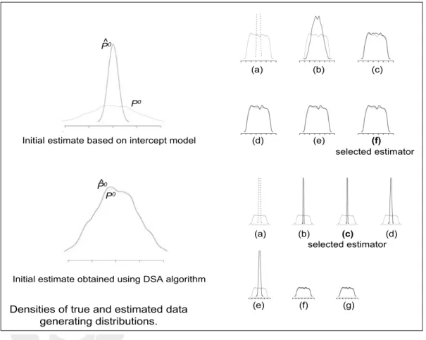
Figure 1 illustrates the collaborative nature of the construction of a se-quence of increasingly data-adaptive nuisance parameter estimators,
{gn1, . . . , gKn}, and its relation to the performance of the initial estimator. We generated 5000 observations of O = (W, A, Y) from data generating distribu-tion dP0 =Q0g0 defined as:
logit(g0(A|W)) = .15W1+.1W2+W3−W4
Q0(A, W) = A+ 3W1−6W2+ 4W3 −5W5+ 3W4
where W1 through W5 are independent random variables ∼ N(0,1), Y =
Q0(A, W) +, ∼ N(0,1), and g0 is the conditional density of A given
con-founding variables W = {W1, W2, W3, W4, W5}. We applied the C-TMLE to
estimate the effect of binary treatment A on outcome Y, adjusting for W, defined as ψ0 =EW (E(Y |A = 1, W)−E(Y |A = 0, W)).
A kernel density estimator was applied to Y and to the predicted values of two initial estimators ofQ0 =E0(Y |A, W), which we denote with ˆQ0n,poor,
and ˆQ0
n,good, respectively. These estimators were obtained with the D/S/A
algorithm (Sinisi and van der Laan, 2004), a data-adaptive machine learning approach to model selection that was set to search over all second degree polynomials of size six. The kernel density estimates are displayed in plots on the left hand side of the figure.
In addition, we plotted the kernel density estimates of the predicted values of each set of the collaboratively-constructed candidate ˆg estimators, and we can compare them with the density of the true predictionsg0(1|W) =P0(A=
1|W). These are plotted on the right hand side of the figure, overlaid with the density estimator applied to the true values g0(1 | W). When the initial fit
of Q0 is poor, the nuisance parameter estimator gkn converges quickly to g0 in
k, and the selected candidate estimator closely approximates g0. Plots in the
bottom half of the figure shows the behavior of the C-TMLE procedure when Q0n is a good estimate of Q0. When the initial fit of Q0 is good, the nuisance
parameter estimator grows slowly towards g0, and a candidate estimator that
estimates a true treatment mechanism that adjusts for fewer covariates than the true treatment mechanism g0 that was used to generate the data.
Densities of true and estimated data generating distributions. P^0 P0 (d) (e) (f) (a) (b) (c) selected estimator (a) (b) (c) (d) selected estimator (e) (f) (g) P^0 P0
Initial estimate obtained using DSA algorithm Initial estimate based on intercept model
Figure 1: Construction of a sequence of nuisance parameter estimators based on a poor initial fit of the density (top) and a good initial fit for the density (bottom). Kernel estimates of true densities Q0 and g0 are shown in gray.
2.6
Revisiting the additive causal effect example
Recall that the targeted maximum likelihood estimator applied to an esti-mator, Qn, of P(Y = 1 | A, W) is obtained by running a univariate logistic
regression ofY, with offset the initial estimator, on an estimate of the univari-ate clever covariunivari-ate hg0(A, W) = A/g0(1 | W)−(1−A)/g0(0 | W), implied
by the treatment mechanism estimator, using an estimator gn of treatment
mechanism P(A= 1|W).
The collaborative targeted maximum likelihood estimation procedure starts with computing Q0
n, an initial estimator of P(Y = 1 | A, W) using super
learning, and then collaboratively generating a sequence of targeted maxi-mum likelihood estimators. These use increasingly nonparametric estimators ofg0, applied to subsequent targeted maximum likelihood updates of the initial
estimator (as needed to guarantee the monotonicity in fit). In this way the se-quence of constructed targeted maximum likelihood estimators has increasing log-likelihood fit. The selection of the sequence of increasingly nonparametric treatment mechanism estimators was based on maximizing the fit of the cor-responding targeted maximum likelihood estimators of P(Y = 1 | A, W), as outlined in our template, thus very much driven by the outcome data. Like-lihood based cross-validation selects the wished targeted maximum likeLike-lihood estimator, with its paired treatment mechanism estimator, from this sequence. It is assumed that the resulting selection of the estimator ofg0 is
nonparamet-ric enough so that the collaborative double robustness of the efficient influence curve as presented in next section is utilized, and, thereby, that our asymptotic linearity theorem in later section can indeed be applied.
A collaborative targeted maximum likelihood estimator constructed in this manner has made every effort to make the estimator of the additive causal ef-fect as unbiased as possible. If we now construct a set of such collaborative targeted maximum likelihood estimators, possibly indexed by different initial estimators, and different ways of constructing the sequence of targeted max-imum likelihood estimators, we can then select among these estimators the estimator with minimal estimated variance (based on the influence curve). To obtain an honest estimate of the variance of the resulting estimator, just as one obtained honest cross-validated risk of an estimator that internally uses cross-validation, one uses the honest cross-validated variance of the influence curve of the complete estimator, including cross-validating this final selection step that involves minimizing the variance.
3
Collaborative double robustness of
estimating functions in CAR censored data
models
In this section we establish a new kind of collaborative robustness of the class of estimating functions in CAR-censored data models, where, as in van der Laan and Robins (2003), the class of estimating functions is implied by the orthogonal complement of the nuisance tangent space of the target parameter Ψ : M → IRd. This orthogonal complement of the nuisance tangent space equals the space spanned by the gradients of the pathwise derivative of Ψ, and thus includes the canonical gradient/efficient influence curve. The collab-orative robustness result teaches us that the censoring mechanism required to obtain an unbiased estimating function at a mis-specifiedQfor the parameter of interest need not always condition on the whole full data structure. In fact, it teaches us that the better Qapproximates Q0 the less of an adjustment by
full data random variables is necessary for the censoring mechanism to still obtain an unbiased estimating function for the parameter of interest. The precise collaborative property of (Q, g0(Q)) such that P0D(ψ0, g0(Q), Q) = 0
will be explicitly specified, where D represents the estimating function, such as the one implied by the canonical gradient.
3.1
The formal collaborative robustness result
The new form of double robustness we wish to establish is understood as follows. Consider an estimating function D(Ψ(Q), G, Q) for the parameter of interest ψ0 that is indexed by nuisance parameters (G0, Q0), and which is
already known to satisfy the classical double robustness property: for any G under which ψ0 is identifiable from PQ0,G, we haveE0D(ψ0, G, Q) = 0 if either
Q = Q0 or G = G0 (van der Laan and Robins (2003)). Given a Q, we are
interested in the question under what conditional distributionG0δ of censoring
variableC, given a reductionX(δ) ofX, will we still haveP0D(ψ0, G0δ, Q) = 0
and thereby that D is an unbiased estimating function for ψ at this mis-specified Q.
Firstly, we note that P0D(ψ0, G, Q) = P0{D(ψ0, G, Q)−D(ψ0, G, Q0)}+
P0D(ψ0, G, Q0), and the latter term is zero under any G that allows
iden-tifiability of ψ0. Thus, it remains to determine for what G0δ we will have
P0{D(ψ0, G0δ, Q)−D(ψ0, G0δ, Q0)} = 0. This choice of G0δ (e.g., it includes
G0 itself) is not unique but will be dependent on a difference Q−Q0 in the
By the general representation theorem for estimating functions that are orthogonal to the nuisance tangent space of the target parameter (Theorem 1.6, van der Laan and Robins (2003)), one can typically represent an esti-mating function D(ψ0, G, Q) as an Inverse Probability of Censoring Weighted
Estimating functionDIP CW(G, ψ0) plus a functionDCAR(Q, G) in the tangent
spaceTCAR(G) of the censoring mechanism atG. The functionDCAR(Q, G) is
defined as the projection of −DIP CW(G, ψ0) on the tangent space TCAR(G) =
{h(O) : EG(h(O) | X) = 0} of the censoring mechanism when only
assum-ing coarsenassum-ing at random, where this projection is carried out in the Hilbert space of all functions of O with mean zero and finite variance endowed with inner product the covariance operator hf1, f2i=EQ,gf1(O)f2(O). In other
in-stances, the DIP CW might depend on Q0 through another parameter beyond
ψ0, in which case it will need to be assumed that this parameter is correctly
specified.
This teaches us that P0{D(ψ0, G, Q)−D(ψ0, G, Q0)}=P0{DCAR(Q, G)−
DCAR(Q0, G)}, since the IPCW-difference equals zero. This representation
theorem also teaches us that for all Q we have that DCAR(Q, G) has
condi-tional mean zero underG, givenX. In addition, this same theorem also shows that Q → DCAR(Q, G) is linear in Q. Therefore, it remains to show that
P0DCAR(Q−Q0, G) = 0. Now, inspection of the proof that the conditional
mean of DCAR(Q0, G) under G equals zero for a Q0 involves typically
condi-tioning on a rich enough reduction ofX so that a particular function indexed by Q0 is fixed under the conditioning. Thus, the censoring mechanism only needs to condition on a particular function of Q−Q0.
This is best illustrated with a concrete censored data structure. For exam-ple, consider the right censored data structures O = (C,X¯(C)), where X(t) is a time dependent process, X = (X(t) : t) represents the full data structure, and ¯X(t) = {X(s) : s ≤ t} represents the sample path up till time t. For this censored data structure, one can represent the projection of DIP CW onto
TCAR as DCAR(Q, G) = R
HQ,G(u,X¯(u−))dMG(u), where
HQ,G(u,X¯(u−)) =EQ,G(DIP CW,G |C =u,X¯(u))−E(DIP CW,G |C ≥u,X¯(u))
dMG(u) = I(C =u)−I(C≥u)dΛC|X(u|X),
and ΛC|X is the cumulative hazard ofC, givenX. For details, we refer to
chap-ter 3 in van der Laan and Robins (2003). HeredMG(u) is a Martingale
satisfy-ing E(dMG(u)|X¯(u), C ≥u) = 0. Due to the linearity of the conditional
ex-pectation operator, we have DCAR(Q−Q0, G) =
R
HQ−Q0,G(u,X¯(u))dMG(u).
By conditioning onHQ−Q0,G(u,X¯(u)) within the integral, and usingE(dMG(u)|
¯
under a censoring mechanism s.t. λC(u | X) only depends on ¯X(u) (it
only depends on ¯X(u) by CAR) through HQ−Q0,G(u,X¯(u)). One can
fac-torize HQ−Q0,G = H1(G)H2(Q −Q0), so that adjustment in λC(u | X) by
the time-dependent covariate H2(Q−Q0)(u,X¯(u)) suffices. Alternatively, it
also suffices if the censoring mechanism uses a self-iterated adjustment by HQ−Q0,G as described later in this section. If Q approximates Q0, this
func-tionHQ−Q0,G(u,X¯(u)) will be shrunk to zero, so that less conditioning becomes
necessary.
The following much simpler (but in essence making the same point) ex-ample helps to further illustrate the general collaborative double robustness property of the efficient influence curve. Suppose the observed censored data structure isO = (W,∆,∆Y) andX = (W, Y) is the full data random variable, where ∆ is the censoring variable. Suppose one wishes to estimate ψ0 =E0Y.
The efficient influence curve is given by
D(ψ0,Π0, Q0) =DIP CW(ψ0,Π0) +DCAR(Q0,Π0), where DIP CW(ψ0,Π0) = Y ∆ Π0(W) −ψ0 DCAR(Q0,Π0) = −E(Y |∆ = 1, W) ∆ Π0(W) −1 , Π0(W) = P0(∆ = 1 | W) and Q0(W) = E0(Y | W,∆ = 1). Consider a Q.
We are interested in the question under what conditional distribution Π0δ of
∆, given a reduction W(δ) of W, will we still have P0D(ψ0,Π0δ, Q) = 0 and
thereby that D is an unbiased estimating function for ψ at this mis-specified Q. Firstly, we note that P0D(ψ0,Π, Q) =P0{D(ψ0,Π, Q)−D(ψ0,Π, Q0)}+
P0D(ψ0,Π, Q0), and the latter term is zero under any Π for whichP0(Π(W)>
0) = 1. Thus, it remains to determine for what Π0δ P0{D(ψ0,Π0δ, Q) −
D(ψ0,Π0δ, Q0)}= 0.
This teaches us that P0{D(ψ0,Π, Q)−D(ψ0,Π, Q0)}=P0{DCAR(Q,Π)−
DCAR(Q0,Π)}, since the IPCW-difference equals zero:
P0{D(ψ0,Π, Q)−D(ψ0,Π, Q0)}=
(Q−Q0)(W)
Π0(W)
(∆−Π0(W)).
Note that we used here that Q → DCAR(Q,Π) is linear in Q. Therefore, it
remains to show that P0DCAR(Q−Q0,Π) = 0. This can be represented as
H(Q−Q0,Π0)(W)(∆−Π0(W)) as above, with H(Q−Q0,Π0)(W) = (Q−