University of California, Berkeley
U.C. Berkeley Division of Biostatistics Working Paper Series
Year Paper
Variable Importance and Prediction Methods
for Longitudinal Problems with Missing
Variables
Ivan Diaz∗ Alan E. Hubbard†
Anna Decker‡ Mitchell Cohen∗∗
∗Department of Biostatistics, Johns Hopkins School of Public Health, [email protected]
†Division of Biostatistics, School of Public Health, University of California, Berkeley,
‡Division of Biostatistics, School of Public Health, University of California, Berkeley,
∗∗Department of Surgery, University of California, San Francisco, [email protected]
This working paper is hosted by The Berkeley Electronic Press (bepress) and may not be commer-cially reproduced without the permission of the copyright holder.
http://biostats.bepress.com/ucbbiostat/paper318 Copyright c2013 by the authors.
Variable Importance and Prediction Methods
for Longitudinal Problems with Missing
Variables
Ivan Diaz, Alan E. Hubbard, Anna Decker, and Mitchell Cohen
Abstract
In this paper we present prediction and variable importance (VIM) methods for longitudinal data sets containing both continuous and binary exposures subject to missingness. We demonstrate the use of these methods for prognosis of medical outcomes of severe trauma patients, a field in which current medical practice in-volves rules of thumb and scoring methods that only use a few variables and ignore the dynamic and high-dimensional nature of trauma recovery. Well-principled prediction and VIM methods can thus provide a tool to make care decisions in-formed by the high-dimensional patient’s physiological and clinical history. Our VIM parameters can be causally interpreted (under causal and statistical assump-tions) as the expected outcome under time-specific clinical interventions. The targeted MLE used is doubly robust and locally efficient. The prediction method, super learner, is an ensemble learner that finds a linear combination of a list of user-given algorithms and is asymptotically equivalent to the oracle selector. The results of the analysis show effects whose size and significance would have been not been found using a naive parametric approach, as well as improvements of up to 0.07 in the AUROC.
1
Introduction
A primary goal in evidence-based medicine is to design prognosis tools that take into account a possibly large set of measured characteristics in order to predict a patient’s most likely medical outcome. An equally important goal is to establish at each given time point which of those measured characteristics is decisive in the development of the predicted outcome. In the statistics literature these two goals have been called prediction and variable importance analysis, respectively. In addition to understanding the underlying biological mechanisms related to positive medical outcomes, the joint use of these tools can help doctors devise the optimal treatment plan according to the specific characteristics of the subject, simul-taneously taking into account hundreds of variables collected for each patient. Despite the current ability to measure a patient’s clinical history in detail, medical practice still involves care decisions based on physician’s experience and rules of thumb that use only a few vari-ables and therefore fail to take into consideration the possible intricate relations between all the measured underlying factors that determine a patient’s health status. In the last years researchers in the fields of biostatistics and bioinformatics have become increasingly more interested in developing mathematical and computational tools that help make optimal care decisions based on all the collected information about a patient’s health status and history which are currently beyond the computational ability of the clinician at the bedside. Because of the large number of variables and the complexity of the relations between them, predic-tion and variable importance would be impossible to achieve without the use of complex statistical algorithms accompanied by powerful computers able to carry out a large number of computations in large data sets within reasonable time frames that help doctors make the right treatment decisions in a timely fashion.
From a technical and practical point of view prediction and variable importance are different goals whose optimal achievement requires the use of different tools. The objective in prediction is to specify a well defined algorithm that is capable of doing accurate predictions, where accuracy can be defined in a variety ways. For prediction it is only relevant whether the prediction algorithm is accurate or not, it is unnecessary to use the intermediate calculations of the algorithm to find statistical or causal relations between the variables involved. In fact, variable importance measures defined in terms of these calculations are often inappropriate (e.g., with parametric models or non-probabilistic predictors), since their validity depends on correctness of the model assumed or their statistical aptness is tied to certain conditions (e.g., empirical process conditions) that may not be known. On the other hand, variable importance (VIM) methods are aimed to measure the degree to which changes in the prediction are caused by changes in each of the predictor variables. VIM methods often provide a ranking of the most likely causes of a the predicted outcome, and are intended to supply doctors with tools for making treatment decisions. This difference between prediction and VIM has two main consequences. First, VIM problems are of a causal nature, whereas prediction problems are merely associational. Second, in order to help the decision making process, VIM parameters must be as informative as possible, having an interpretation in terms of the expected change in the outcome under a given intervention. As explained below, a meaningful interpretation can only be obtained through an intelligible characterization of VIM as a statistical (or causal)
parameter defined as a mapping from a honest, tenable statistical model into an Euclidean space.
Current practice in biostatistics and bioinformatics involves the use of machine learning algorithms for prediction and the posterior computation of VIM quantities based on its output and intermediate calculations (see e.g., Breiman, 2001; Olden and Jackson, 2002; Olden et al., 2004; Strobl et al., 2007, for discussions on random forests and neural networks variable importance). Because these measures are defined in terms of an algorithm that was targeted to perform well at prediction, they result in variable importance measures that can seldom be considered estimates of a well defined causal or statistical parameter. As an example, consider the case of regression and classification trees (e.g., random forests), where the VIM for a variable X is defined as the difference between prediction error when X is perturbed versus the prediction error otherwise (Breiman, 2001; Ishwaran, 2007). The relevance of this quantity as a measure of VIM is unclear because: 1) it does not represent a statistical or causal parameter, 2) it does not have an interpretation in terms of the mechanistic process that generates the data, and 3) its interpretation may be difficult to communicate to the public, even the public trained in statistics. As an example of the technical difficulties arising from this practice, Strobl et al. (2007) discuss the “bias” of random forest VIM measures, missing the fact that bias can only be defined in terms of a target statistical parameter, which is never specified in random forest VIM analysis. Additionally, no formal inference (p-values) methods exist for regression and classification trees based VIM.
Furthermore, an algorithm designed to perform well at prediction is not guaranteed to also do a good job at estimating VIM measures, because good performance is defined differ-ently for each goal. Performance in prediction is typically assessed through quantities like the area under the ROC, the false positive rate, or the expected risk of a sensible loss function. Performance in estimation of Euclidean parameters is assessed in terms of statistical proper-ties like consistency and efficiency (related to bias and variance). Prediction algorithms are designed to perform well at estimating the entire regression model, resulting in an incorrect bias-variance trade-off for each VIM measure.
However, defining VIM parameters in terms of causal relations for continuous variables poses additional technical challenges. When researchers using causal inference methods are faced with exposures of continuous nature, the most common approach is to dichotomize the continuous exposure and consider the effect of its binary version on the outcome. This approach suffers from various flaws. First, the causal parameter does not answer questions about plausible modifications to the data generating mechanism. Stitelman et al. (2010) show that the additive causal effect of a dichotomized exposure compares an intervention in which the density of the exposure is truncated below the dichotomization threshold with an intervention in which the density is truncated above it. Such interventions are seldom realistic, and might not be of great interest for specific applications. Second, even if trun-cation interventions are realistic, the data analyst still has to choose a cutoff point for the dichotomization. Most of the times the decision about such cutoff point is data-driven (i.e., comparing quantiles), or made completely arbitrarily. This practice renders a parameter that is dependent on the data, making its interpretation in terms of the original, continuous expo-sure even more difficult. For instance, if VIM meaexpo-sures for continuous outcomes are defined
in terms of a dichotomization, it is often possible to define the right cutoff point that makes the continuous variable more important than a given binary variable of reference. It is thus necessary to argue why the chosen cutoff point makes these VIM measures comparable.
In this paper we explore a VIM problem in which it is necessary to rank a list of both continuous and binary variables in terms of their importance for developing a medical out-come, which is a very common problem in variable importance analysis. We use state of the art methods for causal inference to solve prediction and VIM problems and illustrate the use of our methods using a medical application, but the methods we develop and the arguments we present are completely general and can be applied to any prediction or VIM problem (e.g., the analysis of ecological data, genomics, educational and social research, economics). For prediction, we use a machine learning technique called super learning , which uses cross validation to choose an optimal convex combination of a list of prediction algorithms pro-vided by the user. The properties of this method have been extensively studied through analytical calculations as well as simulations by van der Laan and Dudoit (2003) and van der Laan et al. (2004, 2007), among others. We define VIM measures in terms of appropriate interventions in a causal model, which results in parameters that have a clear interpretation in terms of the expected outcome under a clinical intervention. VIM measures with causal interpretation are more relevant than their machine learning/modeling counterpart because they attempt to discover the factors that must be intervened upon in order to obtain a signifi-cant improvement in the outcome, and not just the factors that are associated to the outcome in question. We define VIM measures that respect the continuous or binary nature of the variable, and are comparable in the sense that their mathematical definition is equal up to first order, providing a valid ranking of the variables in terms of their causal importance. In order to find VIM estimators with the best possible statistical properties we use the tools for efficient inference in semi-parametric models described by Bickel et al. (1997); van der Laan and Robins (2003), and van der Laan and Rose (2011) among others, which allow us to use asymptotically linear estimators of the VIM parameters that are consistent and efficient in the non-parametric model (under regularity conditions).
We demonstrate the use of these techniques in an example predicting clinical outcomes and evaluating the VIM of a set of competing variables in severe trauma patients. Trauma is the leading cause of death between the ages of 1 and 44, according to the World Health Organization. The vast majority of these deaths take place quickly and much of the initial resuscitative and decision-making action takes place in the first minutes to hours after injury (Hess et al., 2006; Holcomb et al., 2007). In addition, it is clear that as patients progress through their initial resuscitation, the relative attention paid to different physiologic and biologic parameters and indeed the interventions themselves are dynamic. Different variables are important and drive future outcome in the first 30 minutes after injury than at 24 hours when a patient has survived long enough to receive large volume resuscitation, operative intervention and ICU care. While these dynamics are intuitive, most practitioners do not have the ability to know which parameters are important at any given time point. As a result, often the same vital signs and markers are followed throughout the patient’s hospital course independent of whether they are currently relevant. This results in practitioners who are often left making care decisions without knowledge of the current patient physiologic
state and which parameters are important at that moment. Left with this uncertainty and awash in constantly evolving multivariate data, practitioners make decisions based on clinical gestalt, a few favorite variables, and rules of thumb developed from clinical experience. To aid in prediction, the medical literature is filled with scoring systems and published associ-ations between these variables (physiology, biomarker, demographic, etc.) and outcomes of interest (Krumrei et al., 2012; Lesko et al., 2012; MacFadden et al., 2012; Nunez et al., 2009; Sch¨ochl et al., 2011). While numerous, these published statistical associations, given the re-ported methodology, often report misspecified and overfit models. In addition most of these statistical predictive models do not account for the rapidly changing dynamics of a severely injured patient, and fail to take into account the statistical issues discussed in the previous paragraphs. An ideal system would mimic the clinical decision making of an experienced practitioner by providing dynamic prediction (changing prediction at iterative time points) while evaluating the dynamic importance of each variable over time (Buchman, 2010). This then would mimic the implicit understanding a clinician brings to a patient where it is clear that the necessary focus of care must change over time.
The paper is organized as follows. In section 2 we describe the structure of the data and introduce the statistical problem using causal inference tools to define statistical parameters that measure the importance of a variable with respect to an outcome of interest. In section 3 we present various estimators for the variable importance parameters previously defined, and briefly describe the super learner (van der Laan et al., 2007), an ensemble learner whose asymptotic performance is optimal for prediction. In section 4 we describe the problem of prognosis for trauma patients and the dynamic importance of clinical factors, demonstrate the use of the methods previously presented, and compare the results with an approach that utilizes stepwise regression to estimate VIM measures and provides a comparison with common statistical practice. Finally, in section 5 we provide some concluding remarks.
2
Data, problem formulation, and parameters of
inter-est
In order to estimate the effect of a variable A on an outcome Y controlling for a set of variables W, it is common practice among data analysts to estimate the parameter β in a parametric regression model E(Y|A, W) =m(A, W|β) for a known functionm, for example,
E(Y|A, W) =β0+β1A+β2W. (1) It is also common to assume more complex models for the relation between (A, W) and Y
(e.g., by varying the amount of interaction terms, functional form ofm, or by using smoothing techniques), but the linear regression example suffices to introduce the problem. Under model (1), the estimate of β1 is interpreted as the expected change inY given a change of one unit in A:
β1 =E{E(Y|A+ 1, W)−E(Y|A, W)}. (2) Under small violations to the assumptions of model (1) the estimate of β1 cannot be inter-preted as in (2) anymore, therefore we note that the interest of the researcher is to estimate
the right hand side of this equation, not β1. Consider for example the following models:
E(Y|A, W) =β0(1)+β1(1)A+β2(1)W +β3(1)AW (3)
E(Y|A, W) =β0(2)+β1(2)log(A) +β2(2)W. (4) If the true conditional expectation is given by model (3), but (1) is estimated instead, neither the estimate of β1 in model (1) nor β
(1)
1 in (3) represent the quantity in the right hand side of (2), which is now given by β1(1)+β3(1)E(W). On the other hand, if the true model is (4), the parameter of interest is now given by β1(2){E(log(A+ 1))−E(logA)}.
In order to avoid these flaws, in this paper we will define parameters in terms of char-acteristics of the probability distribution of the data under a non-parametric model, as in equation (2). This practice allows the definition of the parameter of interest independently of (possibly) misspecified parametric models, and avoids dealing with different interpretations of regression parameters under incorrect model specifications.
The causal interpretation of statistical parameters (e.g., equation (2)) requires additional untestable assumptions about the distribution of counterfactual outcomes under a hypotheti-cal interventions that are often encoded in a structural equation model (NPSEM Pearl, 2000). In the remaining of the section we will describe the observed data, and define the variable importance measures. We will now introduce the example that motivated the development of these tools, and that will be analyzed in section 4. Since there is little knowledge about the causal structure of these data, we will introduce the variable importance measures by defin-ing them in terms of predictive variable importance. We will then provide the assumptions (NPSEM) that must be met in order to give them a causal interpretation. If the assumptions in the NPSEM do not hold, the estimates do not have a causal interpretation and must not be used to make treatment decisions. In that case, there are two main uses of these estimates. First, they can be used as tools for determining the best set of predictors variables by ruling out those whose with a zero non-significant variable importance. Second, they may be used as a tool for formulating causal hypothesis that may be tested in a subsequent randomized study or in an observational study in which the necessary causal assumptions are met.
Example. The data analyzed in this example were collected as part of the Activation
of Coagulation and Inflammation in Trauma (ACIT, see e.g., Bir et al., 2011; Cohen et al., 2009a,b) study, which is a prospective cohort study of severe trauma patients admitted to a single level 1 trauma center. Several physiological and clinical measurements were recorded at several time points for each patient after arrival to the emergency room. These variables include demographic variables (e.g., age, gender, etc.), baseline risk factors (e.g., asthma, chronic lung disease, Glasgow coma scale, diabetes, injury mechanism, injury severity score, etc.), longitudinally measured variables that account for the patient’s treatment and health status history (e.g., respiratory and heart rate, platelets, coagulation measures like prothrom-bin time and INR, activated protein C, etc.), and an indicator of the occurrence of death at each time interval. Because these data are often collected in a high-stress environment, it is common that some variables are missing for some patients at a given time point. The list of variables we analyzed presented in Appendix A.
and let T denote the time of death of a patient. The observed data for each patient is given by the random variable
O= (L0, C1, L1, Y1, . . . , CJ, LJ, YJ),
where L0 denotes a set of baseline variables recorded at admission to the hospital, Lj =
(Lj1, . . . , LjK) denotes a set of variables measured at time tj, Cj = (Cj1, . . . , CjK) where Cjk
denotes an indicator of missingness of Ljk, and Yj =I(tj < T ≤ tj+1) denotes an indicator of death occurring in the interval (tj, tj+1], for j = 0, . . . , J − 1. Once death occurs the random variables in the remaining time points of the vector O become degenerate so that this structure is well defined.
For the analysis of the ACIT data we have classified the variablesLjk in two non-mutually
exclusive categories: baseline and treatment variables. Baseline variables (L0) are causally related to the outcome but can seldom be manipulated by the physician and are rarely of interest as possible care targets. Although baseline variables are not of interest in themselves, controlling for them is crucial when estimating the effect of treatment variables, which are often longitudinal variables that represent possible targets for clinical care. The label of each variable according to this classification is shown in Table 3 of Appendix A.
We will define VIM measures in terms of the effect of Ljk on Yj0, for all j0 ≥ j and for all k. That is, we are interested in importance of a variable recorded at time point tj on
the hazard of death in each of the subsequent time intervals (tj, tj+1], . . . ,(tJ−1, tJ]. This
approach has the advantage that VIM can be seen as a dynamic process in which the factors that are decisive for developing/predicting a clinical outcome change as a function of time. The problem of variable importance for these data can thus be transformed into a series of cross-sectional problems as follows. For each patient still at risk at tj0, denote
A≡Ljk C ≡Cjk (5) W ≡(L0, Cj−1, Lj−1) Y ≡Yj0, and ¯ Q(A, C, W)≡E(Y|A, C, W), g(A|C, W)≡P(A|C, W) φ(C|W)≡P(C|W), QW(W)≡P(W).
Without loss of generality we will assume that the variable A is either binary or continuous in the interval (0,1). Recall that
E(Y) = EQW Eφ{Eg[ ¯Q(A, C, W)|C, W]}|W
. (6)
IfAis continuous it is possible to replace the conditional densityg(A|C, W) byg(A−δ|C, W), and the probability of missingness φ(C|W) by I(C = 1), obtaining
We define the variable importance measure for continuous variables as
Ψc( ¯Q, QW, g)≡EWEg{Q¯(A+δ,1, W)|C = 1, W} −E(Y), (7)
Indeed, this is a reasonable measure of conditional dependence, since for (A, C)⊥⊥ Y|W we have Ψc( ¯Q, QW, g) = 0. On the other hand, Ψc( ¯Q, QW, g)6= 0 measures the amount in which
small changes of δ inAaffect the expectation of the outcome. Likewise, variable importance measures for binary variables are defined as
Ψb( ¯Q, QW, g)≡EWEg{Q¯(A, C, W)|C = 1, W}+δ{E[ ¯Q(1,1, W)−Q¯(1,0, W)]} −E(Y), (8)
where the first two terms come from replacingg(A|C, W) byg(A|C, W)+(−1)Aδandφ(C|W)
by I(C = 1) in equation (6). The true value of these parameters will be denoted ψc,0 and
ψb,0, respectively.
Comparability We argue that the previous variable importance measures for continuous
and binary variables are comparable up to first order. First of all, note that, under the appropriate differentiability assumptions, for continuous A we have
Ψc( ¯Q, QW, g)≈EW{Q¯(A,1, W)|C = 1, W}+δ d dδEWE{ ¯ Q(A+δ,1, W)|C = 1, W} δ=0 .
This expression and (8) both have the forma+δ×b, whereb can be seen as the appropriate slope of E{Q¯(A, C, W)} as a function of its first argument, providing an argument that, at least in first order, these two VIM measures are comparable.
Underlying causal model In order to give a causal interpretation to the parameters
defined in the previous paragraphs, a series of assumptions about the structure of the data generating process must be true. We will present those assumptions in terms of a non-parametric structural equation model (NPSEM Pearl, 2000), given by
L0 =fL0(UL0)
Cjk =fCjk(Cj−1, Lj−1, L0, UCj) j = 1, . . . , J; k= 1, . . . , K
Ljk =CjkfLjk(Cj−1, Lj−1, L0, ULj) j = 1, . . . , J; k= 1, . . . , K (9)
Yj =fYj( ¯Cj,L¯j, L0, UYj) j = 1, . . . , J,
where, for a random variable X, fX denotes an unknown but fixed function, UX denotes all
the unmeasured factors that are causally related to X, and ¯Xj = (X1, . . . , Xj) denotes the
history of X up until time tj. As pointed out by Pearl (2000), this model assumes that the
data O for each patient are generated by the mechanistic process implied by the functions
fXj with a temporal order dictated by the ordering of the time points tj. In addition, this
NPSEM encodes two important conditional independence assumptions:
Ljk ⊥⊥Ljk∗|(L0, Lj−1) ∀j, k∗ 6=k, (10)
Assumption (10) means that the variables Ljk at time tj are drawn simultaneously as a
function of the past only, and that contemporary variables do not interact with each other. This is a very strong assumption for which there is no support in the severe trauma literature: the causal structure between variables measured contemporaneously is not well understood yet. Assumption (11) means that the value of a variableLjk is only affected by the immediate
past, and is not directly affected by any of the variables measured before or on time tj−2. As a consequence of these assumptions, the problem of estimating the causal effect of each Ljk on each Yj0 for j0 ≥j can be seen as a series of cross-sectional problems as follows. Note that Ljk∗ for k∗ 6= k are not confounders of the causal relation between Ljk and Yj0. To illustrate this, consider the NPSEM encoded in the directed acyclic graph of Figure 1, in which for simplicity we assume that all covariates are observed (i.e., C variables are not present) and that J = K = 2. It stems from the graph that the variable L22 plays no role as a confounder of the causal effect of L21 on Y2. Thus, for fixed j, j0 ≥ j, and k, and for
L0
L11
L12 L21
L22
Y1 Y2
Figure 1: Directed acyclic graph, the arrows in blue and red denote the relations that con-found the causal effect of L21 onY2
each patient still at risk attj0, using the notation introduced in (5), it suffices to consider the following simplified NPSEM:
W =fW(UW), C =fC(W, UC), A=CfA(W, UA), Y =fY(A, C, W, UY), (12)
where the U variables denote all the exogenous, unobserved factors associated to each of the observed variables, and the functions f are deterministic but unknown and completely unspecified. Some additional consequences of NPSEM (12) are:
(1) The missingness indicator C is allowed to depend on the covariates measured in the previous time point. In this way we take into account that a variable can be missing as a result of the previous health status of the patient, and also that it can be strongly correlated with previous missingness indicators.
(2) Missingness is informative. A patient’s missingness indicator C is allowed to affect the way Y is generated, therefore acknowledging that missingness can contain information about the health outcome (e.g., sicker patients who will die earlier might be more likely
to have missing values because information stops being recorded during life-threatening situations).
Continuous Variables. Consider an intervened system in which the variables are
gener-ated by the following system of equations
W =fW(UW)
CI = 1
AI =fA(W, UA) +δ (13)
YI =fY(AI, CI, W, UY),
which, for a small positive δ, can be interpreted as a model in which there is no missingness, and the distribution of the exposure variableAI is shifted to the right byδunits. This type of intervention has been previously discussed in the literature (D´ıaz and van der Laan, 2011a), and belongs to a wider class of interventions known as stochastic interventions (Korb et al., 2004; Didelez et al., 2006; Dawid and Didelez, 2010). The parameter E(YI)−E(Y) can be causally interpreted as the expected reduction in mortality rate gained by an increase of δ
units in the variable A for each patient. Since the counterfactual data OI = (W, CI, AI, YI) are not observed,E(YI) is not estimable without further untestable assumptions. Under the randomization assumption (see, e.g., Rubin, 1978; Pearl, 2000) that
(C, A)⊥YI|W, (14)
and the positivity assumption
g0(A|W)>0, and φ0(1|W)>0 for allA and W , (15) the expectation E(YI) is identified as E(YI) = EWE{Q¯(A + δ, C, W)|C = 1, W}, and
the parameter of interest is defined as (7). A proof of this result under the randomization assumption is presented by D´ıaz and van der Laan (2011a). That proof follows the arguments for identification of general causal parameters given by Pearl (2000), who provides a unified framework for identification of counterfactual parameters as function of the observed data generating mechanism.
Binary Variables For binary variables, following the structural causal model described in
(12), the VIM parameter is defined according to the following intervened system:
W =fW(UW) CI = 1 AI = ( 1 with probabilityg(1|1, W) +δ 0 with probabilityg(0|1, W)−δ YI =fY(AI, CI, W, UY),
where 0 < δ < supwg(0|1, w) is a user-given value. Under randomization assumption (14), and the positivity assumption
0< g0(1|W)<1, and φ0(1|W)>0 for all W , (16) the expectation ofYI is identified as a function of the observed data generating mechanism as
E(YI) =E
WE{Q¯(A, C, W)|C = 1, W}+δ{E[ ¯Q(1,1, W)−Q¯(1,0, W)]}, and the parameter
of interest is defined as (8).
In the following sections we will discuss double robust estimation methods for these pa-rameters.
3
Estimation and prediction methods
We will first discuss the consistent and efficient estimation of the VIM parameters defined in the previous section, and then we will proceed to discuss prediction methods for ¯Q0, g0 and
φ0.
3.1
VIM estimation
In order to define semi-parametric VIM estimates that have optimal asymptotic properties we first need to talk about the efficient influence function. The efficient influence function is a known function D of the data O and P0, and is a key element in semi-parametric efficient estimation, since it defines the linear approximation of all efficient regular asymptotically linear estimators (Bickel et al., 1997). This means that the variance of the efficient influ-ence function provides a lower bound for the variance of all regular asymptotically linear estimators, analogously to the Cramer-Rao lower bound in parametric models. The efficient influence functions of parameters Ψc and Ψb are presented in Appendix B.
We will use targeted minimum loss based estimators (TMLE, van der Laan and Rubin, 2006; van der Laan and Rose, 2011) of the parameters Ψcand Ψb. TMLE is a
substitution/plug-in estimation method that, given substitution/plug-initial estimators ( ¯Qn, QW,n, gn) of ( ¯Q, QW, g), finds updated
estimators ( ¯Q∗n, Q∗W,n, gn∗) and defines the estimator of Ψ as
ψn = Ψ( ¯Q∗n, Q
∗
W,n, g
∗
n).
TMLE is an estimation method that enjoys the best properties of both G-computation es-timators (Robins, 1986) and the estimating equation methodology (see e.g., van de Geer, 2000; van der Laan and Robins, 2003). On one hand, TMLE is similar to G-computation estimators (e.g., Ψ( ¯Qn, QW,n, gn)) in that it is a plug-in estimator, and therefore produces
estimates that are always within the range of the parameter of interest (e.g., it is always in the interval [0,1] if the estimand is a probability). On the other hand, under regularity conditions and consistency of ( ¯Qn, gn, φn), it is asymptotically linear with influence function
equal to the efficient influence function:
ψn−ψ0 = n X i=1 D(P0)(Oi) +oP(1/ √ n).
As a consequence, TMLE has the following properties: • It is a substitution/plug-in estimator.
• It is efficient if ¯Qn, gn, and φn are consistent for ¯Q0, g0, and φ0, respectively.
• It is consistent if either ¯Qn or both gn and φn are consistent. This property is referred
to as double robustness.
• It is more robust to empirical violations of the positivity assumptions (15) and (16). In Appendix B we describe an iterative procedure that transforms the initial estimates ¯Qnand
gninto targeted estimates ¯Q∗nandg
∗ nsuch that Ψ( ¯Q ∗ n, g ∗ n, Q ∗ W,n) is a TMLE of Ψ( ¯Q0, g0, QW,0), and discuss in more detail the properties of the TMLE. An R function that computes the TMLE of ψ0 can be found in http://works.bepress.com/ivan_diaz/5/.
Estimating equation (EE), Gcomp/IPMW, and unadjusted estimators In
addi-tion to the TMLE we will compute three addiaddi-tional estimates of the VIM, for comparison with other estimation methods. The first estimator, the estimating equation (EE) method-ology, is an estimator that uses the efficient influence function of the parameter in order to define the estimator as the solution of the corresponding estimating equation. Because the EE is also asymptotically linear with influence function equal to the efficient influence function, it is consistent and asymptotically efficient. However, the estimating equation that defines the EE may not have a solution in the parameter space, in which case the EE does not exist. The second estimator, a mixture of the G-computation formula and the inverse probability of missingness weighted estimator IPMW (Gcomp/IPMW) represents a choice that could have been made in common practice in statistics. The Gcomp/IPMW estimator uses initial estimators φn and ¯Qn of φ0 and ¯Q0 obtained through step-wise regression, and is defined as ψc,n,GI = 1 n n X i=1 Ci φn(Wi) ¯ Qn(Ai+δ,1, Wi)−Yi ψb,n,GI = 1 n n X i=1 Ci φn(Wi) ¯ Qn(Ai,1, Wi) +δ[ ¯Qn(1,1, Wi)−Q¯n(0,1, Wi)]−Yi ,
for Ψc and Ψb, respectively. This estimator is consistent only if both the model for φ0 and the model for ¯Q0 have been correctly specified. The unadjusted estimator is identical to the Gcomp/IPMW estimator but including only the intercept term in the vector W.
Since the consistency of the initial estimators of ¯Q0, g0 and φ0 is key to attain estimators with optimal statistical properties (i.e., consistency and efficiency), we will carefully discuss the construction of such estimators in the next subsection. In particular, the next subsection deals with the construction of an estimator for ¯Q0, the predictor of death in our working example.
3.2
Prediction
As explained in the previous section, the consistency of the initial estimators ¯Qn, gn and ψn
determine the statistical properties of the estimators of ψc,0 and ψb,0. Common practice in statistics involves the estimation of models like
logit ¯Q(A, W) = β0 +β1A+β2W +β3AW. (17)
This approach that has gained popularity among researchers in epidemiology and biostatis-tics, partly because of the analysis of its statistical properties requires simple mathematical methods, and partly because it is readily available in every statistical software. Neverthe-less, as it is also well known among their users, parametric models of the type described by (17) are rarely correct, and their choice is merely based on their computational advantages and other subjective criteria. This practice leads to regression estimator whose usefulness is highly questionable given that the assumptions it entails (linearity, normality, link function, etc.) do not originate in legitimate knowledge about the phenomena under study, but rather come from analytical tractability and computational convenience.
In this paper we will use the super learner (van der Laan et al., 2007) for estimation of ¯Q0,
g0, andψ0. Super learner is a methodology that uses cross-validated risks to find an optimal combination of a list of user-supplied estimation algorithms. One of its most important the-oretical properties is that its solution converges to the oracle estimator (i.e., the candidate in the library that minimizes the loss function with respect to the true probability distribution), thus providing the closest approximation to the real data generating mechanism. Proofs and simulations regarding these and other asymptotic properties of the super learner can be found in van der Laan et al. (2004) and van der Laan and Dudoit (2003).
To implement the super learner predictor it is necessary to specify a library of candidate predictors algorithm. In the case of the conditional expectations ¯Q0, φ0, and g0 for binary A, the candidates can be any regression or classification algorithm. Examples include random forests, logistic regression, k nearest neighbors, Bayesian models, etc. For estimation of the conditional densities g0 we will also use the super learner, with candidates given by several histogram density estimators, which yields a piece-wise constant estimator of the conditional density. The choice of the number of bins and their location is indexed by two tuning parameters. The implementation of this density estimator is discussed in detail by D´ıaz and van der Laan (2011b), and will be omitted in this paper.
4
Data Analysis
In this section we analyze the data described in the example of Section 2. The sample size wasn= 918 patients, and measurements of the variables described in Appendix A were taken at 6, 12, 24, 48, and 72 hours after admission to the emergency room.
The main objective of the study was the construction of prediction models for the risk of death of a patient in a certain time interval given the variables measured up to the start of the interval, as well as the definition and estimation of VIM measures that provide an
account of the longitudinal evolution of the relation between these physiological and clinical measurements and the risk of death at a certain time point.
The data set was partitioned in 6 different data sets according to the time intervals defined by the time points in which measurements were taken, each of these 6 datasets contained only the patients that were at risk of death (alive) at the start of the time interval. Each of the continuous covariates was rescaled by subtracting the minimum and dividing by the range so that all of the covariates range between zero and one. The methods described in the previous sections were applied to each variable in each of these datasets.
The candidate algorithms for prediction of death used in the super learner predictor are as follows:
• Logistic regression with main terms (GLM) • Stepwise logistic regression (SW)
• Bayesian logistic regression (BLR) • Generalized additive models (GAM) • Earth (Earth)
• Sample mean (MEAN),
from which the first three represent common practice in epidemiology and statistics, GAM and Earth are algorithms that intend to capture non-parametric structures of the data, and the sample mean is included for contrast.
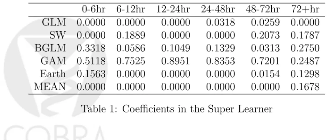
Table 1 shows the coefficients of each candidate algorithm in the super learner predictor of E(Yj|L¯j,C¯j, L0). The variability in these coefficients shows that no single algorithm is optimal for prediction at each time point, and that each algorithm describes certain features of the data generating mechanism that the others are not capable of unveiling.
0-6hr 6-12hr 12-24hr 24-48hr 48-72hr 72+hr GLM 0.0000 0.0000 0.0000 0.0318 0.0259 0.0000 SW 0.0000 0.1889 0.0000 0.0000 0.2073 0.1787 BGLM 0.3318 0.0586 0.1049 0.1329 0.0313 0.2750 GAM 0.5118 0.7525 0.8951 0.8353 0.7201 0.2487 Earth 0.1563 0.0000 0.0000 0.0000 0.0154 0.1298 MEAN 0.0000 0.0000 0.0000 0.0000 0.0000 0.1678
Table 1: Coefficients in the Super Learner
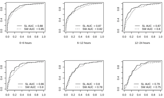
Figure 2 presents the ROC curves for the cross-validated super learning predictions of death, as well as the cross-validated predictions based on a logistic model with AIC-based stepwise selection of variables, for comparison with common practice. The super learner prediction methods outperforms the stepwise prediction in all cases, with AUC ROC (area
under the ROC curve) differences ranging from 0.02 to 0.07. Though this differences might be small, an interpretation of their meaning reveals the clinical relevance of a slight improvement in prediction. The AUC ROC can be interpreted as the proportion of times that a patient who will die obtains a higher prediction score than a patient who will survive. In practice, an AUC ROC difference of 0.02 means that in 100 pairs of patients (pairs formed by one patient who will die and one who will not) the super learner classifier will correctly classify two pairs more than the step-wise classifier, which could potentially lead to live-saving treatments for these two patients.
0−6 hours 0.0 0.2 0.4 0.6 0.8 1.0 0.0 0.4 0.8 SL AUC = 0.88 SW AUC = 0.85 6−12 hours 0.0 0.2 0.4 0.6 0.8 1.0 0.0 0.4 0.8 SL AUC = 0.87 SW AUC = 0.82 12−24 hours 0.0 0.2 0.4 0.6 0.8 1.0 0.0 0.4 0.8 SL AUC = 0.87 SW AUC = 0.8 24−48 hours 0.0 0.2 0.4 0.6 0.8 1.0 0.0 0.4 0.8 SL AUC = 0.86 SW AUC = 0.8 48−72 hours 0.0 0.2 0.4 0.6 0.8 1.0 0.0 0.4 0.8 SL AUC = 0.8 SW AUC = 0.78 72+ hours 0.0 0.2 0.4 0.6 0.8 1.0 0.0 0.4 0.8 SL AUC = 0.79 SW AUC = 0.75
Figure 2: ROC curves of cross-validated prediction for the super learner (SL) and the logistic step-wise regression (SW), for different time intervals.
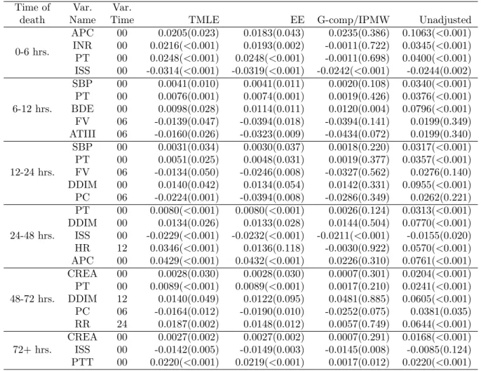
The VIM-TMLE measures that were significant at 0.05 were ranked according to their magnitude. Table 2 presents the first five (whenever five or more were significant) most important variables for prediction of death at each time interval, according to the TML estimator presented in Section 3. Recall that all the continuous variables were re-scaled between zero and one; the value δ = 0.01 was used for all the estimates. The interpretation of the values in the first row of Table 2, for example, is that if APC were to increase by 1% for every patient, the mortality rate in the first time interval would be augmented by 2%. The TMLE and the EE produced generally similar results, whereas the Gcomp/IPMW estimator produced results that are somewhat different and not significant more frequently. Note that several of the Gcomp/IPMW point estimates coincide with the TMLE and EE, but p-values generally larger. This could be due to the fact that the TMLE and EE are efficient estimators, and therefore provide more powerful hypothesis tests. In light of the superior
theoretical properties of the TMLE and EE, we prefer to rely on estimates obtained through these methods.
Time of Var. Var.
death Name Time TMLE EE G-comp/IPMW Unadjusted
0-6 hrs. APC 00 0.0205(0.023) 0.0183(0.043) 0.0235(0.386) 0.1063(<0.001) INR 00 0.0216(<0.001) 0.0193(0.002) -0.0011(0.722) 0.0345(<0.001) PT 00 0.0248(<0.001) 0.0248(<0.001) -0.0011(0.698) 0.0400(<0.001) ISS 00 -0.0314(<0.001) -0.0319(<0.001) -0.0242(<0.001) -0.0244(0.002) 6-12 hrs. SBP 00 0.0041(0.010) 0.0041(0.011) 0.0020(0.108) 0.0340(<0.001) PT 00 0.0076(0.001) 0.0074(0.001) 0.0019(0.426) 0.0376(<0.001) BDE 00 0.0098(0.028) 0.0114(0.011) 0.0120(0.004) 0.0796(<0.001) FV 06 -0.0139(0.047) -0.0394(0.018) -0.0394(0.141) 0.0199(0.349) ATIII 06 -0.0160(0.026) -0.0323(0.009) -0.0434(0.072) 0.0199(0.340) 12-24 hrs. SBP 00 0.0031(0.034) 0.0030(0.037) 0.0018(0.220) 0.0317(<0.001) PT 00 0.0051(0.025) 0.0048(0.031) 0.0019(0.377) 0.0357(<0.001) FV 06 -0.0134(0.050) -0.0246(0.008) -0.0327(0.562) 0.0276(0.140) DDIM 00 0.0140(0.042) 0.0134(0.054) 0.0142(0.331) 0.0955(<0.001) PC 06 -0.0224(0.001) -0.0394(0.008) -0.0286(0.349) 0.0262(0.221) 24-48 hrs. PT 00 0.0080(<0.001) 0.0080(<0.001) 0.0026(0.124) 0.0313(<0.001) DDIM 00 0.0134(0.026) 0.0133(0.028) 0.0144(0.504) 0.0770(<0.001) ISS 00 -0.0229(<0.001) -0.0232(<0.001) -0.0211(<0.001) -0.0155(0.020) HR 12 0.0346(<0.001) 0.0136(0.118) -0.0030(0.922) 0.0570(<0.001) APC 00 0.0429(<0.001) 0.0432(<0.001) 0.0226(0.310) 0.0761(<0.001) 48-72 hrs. CREA 00 0.0028(0.030) 0.0028(0.030) 0.0007(0.301) 0.0204(<0.001) PT 00 0.0089(<0.001) 0.0089(<0.001) 0.0017(0.210) 0.0241(<0.001) DDIM 12 0.0140(0.049) 0.0122(0.095) 0.0481(0.885) 0.0605(<0.001) PC 06 -0.0164(0.012) -0.0190(0.010) -0.0252(0.075) 0.0381(0.035) RR 24 0.0187(0.002) 0.0148(0.012) 0.0057(0.749) 0.0644(<0.001) 72+ hrs. CREA 00 0.0027(0.002) 0.0027(0.002) 0.0007(0.291) 0.0168(<0.001) ISS 00 -0.0142(0.005) -0.0149(0.003) -0.0145(0.008) -0.0085(0.124) PTT 00 0.0220(<0.001) 0.0219(<0.001) 0.0017(0.012) 0.0220(<0.001) Table 2: VIM estimates for the most important variables for prediction of death at each time interval according to TML estimate (p-values in parentheses and truncated at 0.001).
In addition to the previous tables, Figure 3 shows heat maps of the VIM measures. For example, Figure 3a shows the importance of each of the variables measured at baseline on the outcome between 0-6 hours, 6-12 hours, 12-24 hours, 24-48 hours, 48-72 hours, and 72+ hours. Additionally, the dendrogram plotted in the left margin of Figure 3a shows a hierarchical clustering of the variables according to the profile of their effect on the longitudinal outcome. At each time point, variables that less than 15% of observed values were not included in the analysis. For this reason, and because missingness was more common in later measurement times, the number of variables included in Figure 3 decreases as the time of measurement increases. Additionally, the output for variables measured at 48 and 72 hours is not shown because none of the results were significant.
* *** *** *** * *** *** *** *** *** * *** * *** *** *** *** *** *** * * * *** *** *** *** *** *** * * * *** *** *** *** *** ***
Hour 00 Hour 06 Hour 12 Hour 24 Hour 48 Hour 72 APC HCT CREA HGB ISS PTT BUN GCS PLTS RR HR SBP INR PT DDIM ATIII FV PC BDE FVIII −0.06 −0.04 −0.02 0 0.02 0.04 0.06
(a) Variables measured at admission
*** * * * *** * *
Hour 06 Hour 12 Hour 24 Hour 48 Hour 72
HR SBP BDE RR APC PC FV FVIII ATIII DDIM −0.02 −0.01 0 0.01 0.02
(b) Variables measured at 6 hours
***
*
Hour 12 Hour 24 Hour 48 Hour 72
HR BDE RR SBP APC DDIM ATIII FV FVIII PC −0.03 −0.02 −0.01 0 0.01 0.02 0.03
(c) Variables measured at 12 hours
*
***
***
Hour 24 Hour 48 Hour 72
BDE DDIM HR RR FV ATIII SBP APC FVIII PC −0.02 −0.01 0 0.01 0.02
(d) Variables measured at 24 hours
Figure 3: VIM estimates of measured variables according to TMLE. ‘***’ indicates p-value ≤ 0.001, ‘**’ indicates 0.001 <p-value ≤ 0.01, and ‘*’ indicates 0.01< p-value ≤ 0.05.
These graphs confirm the hypothesis that the main drivers of recovery after trauma are dynamic over time. For example, the variables in the top of Figure 2 (APC, HCT, CREA, HGB), measured at baseline, do not have an immediate effect on the hazard of death in the first six hours, but result very relevant to predict the outcome between 6 and 24 hours. Note that these variables are mostly related to the coagulation cascade and inflammation. On
the other hand, variables like HR and RR that are related to the general health status of a patient play an important role only when measured 12 after admission.
Due to the severity of the missingness at later time points, it is not possible to perform a comparison of the time trajectory of each variable based on these data. However, these results provide useful tools to formulate hypothesis that may be tested in subsequent studies.
5
Discussion
In this paper we addressed the problem of estimating variable importance parameters for longitudinal data that are subject to missingness. We present variable importance parameters that have a clear interpretation either as purely statistical parameters or as causal effects, depending on the assumptions about the data generating mechanism that the researcher is willing to make. These are important characteristics that advance the field in various fronts. First, unlike VIMs derived from machine learning and data-adaptive predictors (e.g., random forests), the VIMs defined in this paper have a concise definition as statistical parameters, which allowed the study of its mathematical properties and ultimately led to the construction of estimators with desirable statistical properties like consistency and efficiency. Second, the assumptions required to give a causal interpretation to statistical parameters are often concealed, and the language used attempts to imply causal relations without clearly stating the necessary assumptions. The framework we present endows the user with the necessary tools to decide whether it is correct or not to interpret the estimates in terms of causal relations. Additionally, the parameters that we present have a purely statistical interpretation as a measure of conditional dependence, interpretation that must be used when there is not enough knowledge about the causal structure. We provide a methodology that can be used to compare continuous and binary variables in terms of their effect on an outcome, guaranteeing that the results will be mathematically comparable.
We illustrate the use of the methods through the analysis of an example related to recovery after sever trauma, and present the results of the analysis. These analyses provide a significant contribution to the field of trauma injury, by bringing state-of-the-art statistical methods to a field in which the large dimensionality of the problem constitutes a limiting factor for understanding the intricate relations between the variables involved. We propose a “black-box” prognosis algorithm (super learner) that can take into account the complexity of the problem, and represents an alternative to the scoring methods based on rules of thumb that are currently used in this setting. The results of the variable importance analysis corroborate the hypothesis that recovery after severe trauma is a dynamic process in which the decisive factors change over time, and provides provisional answers to various questions about recovery after severe trauma. Because the structural causal assumptions required are not met, the estimated VIMs can only be used as predictive performance measures and used to postulate hypothesis about causal relations that can be tested in more carefully designed studies. An additional advantage of a more carefully designed study is the possibility of performing a detailed comparison of the trajectories of each variable, using data that is not subject to missingness, or in which the amount of missingness is controlled.
We proposed a TMLE and an estimating equation estimator. Both of these estimators are doubly robust and efficient under certain regularity and consistency conditions of the ini-tial estimators, but the TMLE has the theoretical advantage that it is a bounded estimator. However, we did not observe any relevant difference between them in the illustration example. D´ıaz and van der Laan (2011a) have already compared these two estimators through a sim-ulation study under no missingness of the treatment variable, finding no difference between them. We proposed the G-comp/IPMW, an additional estimator that represents an easy al-ternative to the TMLE or EE. Although we found various differences in the magnitude of the estimates between the TMLE and the G-comp/EE, the main discrepancy was with respect to the standard errors and p-values. We hypothesize that these differences are a consequence of the inefficiency of the G-comp/IPMW, which results in hypothesis tests with less power.
Appendix A
The variables analyzed in the ACIT study are presented in Table 3. Variable Type Description
Age Baseline Age in years
GCS Baseline/Treatment Arrival Glascow Comma Score ISS Baseline/Treatment Injury Severity Score
Asthma Baseline Indicator of previous Asthma
COPD Baseline Indicator of previous Chronic Obstructive Pulmonary Disease OCLG Baseline Indicator of Other Chronic Lung Disease
CAD Baseline Coronary Artery Disease CHF Baseline Congestive Heart Failure ESRD Baseline End Stage Renal Disease CIRR Baseline Cirrhosis
DIAB Baseline Diabetes
HPAN Baseline Hypoalbuminemia Gender Baseline Gender
MECH Baseline Injury mechanism: blunt or penetrating HR Treatment Heart Rate
RR Treatment Respiratory Rate
SBP Treatment Spontaneous Bacterial Peritonitis BDE Treatment Base Deficit/Excess
BUN Treatment Blood Urea Nitrogen CREA Treatment Creatinine
HGB Treatment Hemoglobin HCT Treatment Hematocrit PLTS Treatment Platelets
PT Treatment Prothrombin Time PTT Treatment Partial Prothrombin Time INR Treatment International Normalized Ratio FV Treatment Factor III
FVIII Treatment factor VIII ATIII Treatment Antithrombin III PC Treatment Protein C DDIM Treatment D-Dimer
TPA Treatment Tissue Plasminogen Activator PAI Treatment Plasminogen Activator Inhibitor SEPCR Treatment Soluble Endothelial Protein C Receptor STM Treatment Soluble Thrombomodulin
APC Treatment Activated Protein C
Appendix B
The efficient influence function of parameters (7) and (8) are given by
Dc( ¯Q, QW, g, φ)(O) = Dc1( ¯Q, g, φ)(O) +Dc2( ¯Q, g, φ)(O) +Dc3( ¯Q, QW, g)(O) (18) Db( ¯Q, QW, g, φ)(O) = Db1( ¯Q, g, φ)(O) +Db2( ¯Q, g, φ)(O) +Db3( ¯Q, QW, g)(O), (19) respectively, where Dc1( ¯Q, g, φ)(O) = C φ(1|W) g(A−δ|1, W) g(A|1, W) {Y − ¯ Q(A,1, W)} Dc2( ¯Q, g, φ)(O) = C φ(1|W) ¯ Q(1, A+δ, W)−Eg{Q¯(1, A+δ, W)|C = 1, W} (20) Dc3( ¯Q, QW, g)(O) =Eg{Q¯(1, A+δ, W)|C= 1, W} −Y −Ψc( ¯Q, QW, g), and Db1( ¯Q, g, φ)(O) = C φ(1|W) δ 2A−1 g(A|1, W) + 1 {Y −Q¯(A,1, W)} Db2( ¯Q, g, φ)(O) = C φ(1|W)[ ¯Q(A,1, W)−Eg{ ¯ Q(A,1, W)|C = 1, W}] (21) Db3( ¯Q, QW, g)(O) =δ{Q¯(1,1, W)−Q¯(0,1, W)}+Eg{Q¯(A,1, W)|C= 1, W} −Y −Ψb( ¯Q, QW, g).
Result 1 provides the conditions under which these estimating equations have expectation zero, therefore leading to consistent, triply robust estimators.
Result 1. Let D be either Dc or Db presented in equations (18) and (19). We have that
EP0{D(O|φ, g,Q, ψ¯ 0)}= 0
if either (Q¯= ¯Q0 and φ =φ0) or (Q¯ = ¯Q0 and g =g0) or (g =g0 and φ=φ0).
Recall that an estimator that solves an estimating equation will be consistent if the expectation of the estimating equation equals zero. As a consequence of this result, and under the conditions on ¯Q,g andφ stated in Theorem 5.11 and 6.18 of van der Vaart (2002), an estimator that solves the efficient influence function D will be consistent if either two of the three initial estimators are consistent, and it will be efficient if all of them are consistently estimated. Mathematical proofs of the efficiency of these estimators are out of the scope of this paper, but the general theory underlying their asymptotic properties can be found in van der Laan and Robins (2003), among others.
Appendix B.1
TMLE algorithm
In order to define a targeted maximum likelihood estimator for ψ0, we need to define three elements: (1) A loss functionL(Q) for the relevant part of the likelihood required to evaluate
Ψ(P), which in this case isQ= ( ¯Q, g, QW). This function must satisfyQ0 = arg minQEP0L(Q)(O),
where Q0 denotes the true value of Q; (2) An initial estimator Q0n of Q0; (3) A parametric fluctuationQ() throughQ0
n such that the linear span of d
dL{Q()}|=0 contains the efficient
influence curve D(P) defined by either (18) or (19), depending on whether A is continuous or binary. These elements are defined below:
Loss Function
As loss function for Q, we will consider L(Q) =LY( ¯Q) +LA(g) +LW(QW), where LY( ¯Q) =
Y log{Q¯(A, W)} + (1 − Y) log{1 − Q¯(A, W)}, LA(g) = −logg(A|W), and LW(QW) =
−logQW(W). It can be easily verified that this function satisfiesQ0 = arg minQEP0L(Q)(O).
Parametric Fluctuation
Given an initial estimator Qk
n ofQ0, with components ( ¯Qkn, gnk, QkW,n), we define the (k+ 1)th
fluctuation of Qkn as follows: logit ¯Qkn+1(1)(A, W) = logit ¯Qkn(A, W) +1H1k(C, A, W) gkn+1(1)(A|W)∝exp{1H2k(A, W)}g k n(A|W) QkW,n+1(2)(W)∝exp{2H3k(W)}Q k W,n(W),
where the proportionality constants are so that the left hand side terms integrate to one, for continuous A H1k(A, C, W) = C φn(1|W) gk n(A−δ|,1W) gk n(A|,1, W) , for binary A H1k(A, C, W) = C φn(1|W) δ 2A−1 gk n(A|1, W) + 1 ,
H2k(A, W) =D2(Pk)(O), and H3(W) =D3(Pk)(O), with D2 and D3 defined as in (20) and (21). We define these fluctuations using a two-dimensional with two different parameters1 and 2, though it is theoretically correct to define these fluctuations using any dimension for
, as far as the condition D(P)∈< ddL{Q()}|=0 > is satisfied, where <·> denotes linear span. The convenience of the particular choice made here will be clear once the targeted maximum likelihood estimator (TMLE) is defined.
Targeted Maximum Likelihood Estimator
The TMLE is defined by the following iterative process: 1. Initialize k= 0.
2. Estimate ask
n = arg minPnL{Qkn()}.
3. ComputeQk+1
n =Qkn(kn).
First of all, note that the value of2that minimizes the part of the loss function corresponding to the marginal distribution ofW in the first step (i.e.,−PnlogQW,n1 (2)) is12 = 0. Therefore, the iterative estimation of only involves the estimation of1. Thekth step estimation of 1 is obtained by minimizingPn(LY( ¯Qkn(1)) +LA(gnk(1))), which implies solving the estimating equation Sk(1) = n X i=1 Yi−expit{logit ¯Qkn(Ai, Wi) +1H1k(Oi)} H1k(Oi) +D2(Pnk)(Oi)− R AD2(P k n)(Yi, a, Wi) exp{1D2(Pnk)(Yi, a, Ci, Wi)} gnk(a|1, Wi)dµ(a) R Aexp{1D2(Pnk)(Yi, a, Ci, Wi)} gkn(a|1, Wi)dµ(a) (22) where D2(Pnk)(O) = ¯Q k n(A+δ,1, W)− Z A ¯ Qkn(a+δ,1, W)gkn(a|1, W)dµ(a).
The TMLE ofψ0 is defined asψn≡limk→∞Ψ(Pnk), assuming this limit exists. In practice,
the iteration process is carried out until convergence in the values of k is achieved, and an
estimator Q∗n is obtained. Under the conditions of Theorem 2.3 of van der Laan and Robins (2003), a conservative estimator of the variance of ψn is given by
1 n n X i=1 D2( ¯Q∗n, QW,n, gn∗, φn)(Oi).
References
P.J. Bickel, C.A.J. Klaassen, Y. Ritov, and J. Wellner. Efficient and Adaptive Estimation for Semiparametric Models. Springer-Verlag, 1997.
Nastasha Bir, Mathieu Lafargue, Marybeth Howard, Arnaud Goolaerts, Jeremie Roux, Michel Carles, Mitchell J Cohen, Karen E Iles, Jos´e A Fern´andez, John H Griffin, et al. Cytoprotective-selective activated protein c attenuates pseudomonas aeruginosa–induced lung injury in mice. American journal of respiratory cell and molecular biology, 45(3):632, 2011.
Leo Breiman. Random forests. Machine Learning, 45:5–32, 2001. ISSN 0885-6125.
T.G. Buchman. Novel representation of physiologic states during critical illness and recovery.
Crit. Care, 14:127, 2010.
Mitchell Cohen, Karim Brohi, Carolyn Calfee, Pamela Rahn, Brian Chesebro, Sarah Chris-tiaans, Michel Carles, Marybeth Howard, and Jean-Fran¸cois Pittet. Early release of high mobility group box nuclear protein 1 after severe trauma in humans: role of injury severity and tissue hypoperfusion. Critical Care, 13(6):R174, 2009a.
Mitchell J Cohen, Natasha Bir, Pamela Rahn, Rachel Dotson, Karim Brohi, Brian B Chese-bro, Robert Mackersie, Michel Carles, Jeanine Wiener-Kronish, and Jean-Fran¸cois Pittet. Protein c depletion early after trauma increases the risk of ventilator-associated pneumonia.
The Journal of Trauma and Acute Care Surgery, 67(6):1176–1181, 2009b.
A. Philip Dawid and Vanessa Didelez. Identifying the consequences of dynamic treatment strategies: A decision-theoretic overview. CoRR, abs/1010.3425, 2010.
Iv´an D´ıaz and Mark van der Laan. Population intervention causal effects based on stochastic interventions.Biometrics, page In press., 2011a. ISSN 1541-0420. doi: 10.1111/j.1541-0420. 2011.01685.x. URLhttp://dx.doi.org/10.1111/j.1541-0420.2011.01685.x.
Iv´an D´ıaz and Mark van der Laan. Super learner based conditional density estimation with application to marginal structural models. The International Journal of Biostatistics, 7 (1):38, 2011b.
Vanessa Didelez, A. Philip Dawid, and Sara Geneletti. Direct and indirect effects of sequential treatments. In UAI, 2006.
J.R. Hess, J.B. Holcomb, and D.B. Hoyt. Damage control resuscitation: the need for specific blood products to treat the coagulopathy of trauma. Transfusion, 46:685–686, May 2006. J.B. Holcomb, N.R. McMullin, L. Pearse, J. Caruso, C.E. Wade, L. Oetjen-Gerdes, H.R. Champion, M. Lawnick, W. Farr, S. Rodriguez, et al. Causes of death in us special operations forces in the global war on terrorism: 2001–2004. Annals of surgery, 245(6): 986, 2007.
Hemant Ishwaran. Variable importance in binary regression trees and forests. Electronic Journal of Statistics, pages 519–537, 2007.
Kevin. Korb, Lucas. Hope, Ann. Nicholson, and Karl. Axnick. Varieties of causal intervention. In Chengqi Zhang, Hans W. Guesgen, and Wai-Kiang Yeap, editors,PRICAI 2004: Trends in Artificial Intelligence, volume 3157 of Lecture Notes in Computer Science, pages 322– 331. Springer Berlin / Heidelberg, 2004.
N.J. Krumrei, M.S. Park, B.A. Cotton, and M.D. Zielinski. Comparison of massive blood transfusion predictive models in the rural setting. The Journal of Trauma and Acute Care Surgery, 72(1):211, 2012.
M.M. Lesko, T. Jenks, S. O’Brien, C. Childs, O. Bouamra, M. Woodford, and F. Lecky. Comparing model performance for survival prediction using total gcs and its components in traumatic brain injury. Journal of Neurotrauma, (ja), 2012.
L.N. MacFadden, P.C. Chan, K.H.H. Ho, and J.H. Stuhmiller. A model for predicting primary blast lung injury. The Journal of Trauma and Acute Care Surgery, 2012.
T.C. Nunez, I.V. Voskresensky, L.A. Dossett, R. Shinall, W.D. Dutton, and B.A. Cotton. Early prediction of massive transfusion in trauma: simple as abc (assessment of blood consumption)? The Journal of Trauma and Acute Care Surgery, 66(2):346–352, 2009. Julian D Olden and Donald A Jackson. Illuminating “the black box”: a randomization
approach for understanding variable contributions in artificial neural networks. Ecological Modelling, 154:135 – 150, 2002. ISSN 0304-3800.
Julian D Olden, Michael K Joy, and Russell G Death. An accurate comparison of meth-ods for quantifying variable importance in artificial neural networks using simulated data.
Ecological Modelling, 178:389 – 397, 2004. ISSN 0304-3800.
J. Pearl. Causality: Models, Reasoning, and Inference. Cambridge University Press, Cam-bridge, 2000.
J.M. Robins. A new approach to causal inference in mortality studies with sustained expo-sure periods - application to control of the healthy worker survivor effect. Mathematical Modelling, 7:1393–1512, 1986.
D.B. Rubin. Bayesian inference for causal effects: the role of randomization. Annals of Statistics, 6:34–58, 1978.
H. Sch¨ochl, B. Cotton, K. Inaba, U. Nienaber, H. Fischer, W. Voelckel, and C. Solomon. Fibtem provides early prediction of massive transfusion in trauma. Crit care, 15(6):R265, 2011.
Ori M. Stitelman, Alan E. Hubbard, and Nicholas P. Jewell. The impact of coarsening the explanatory variable of interest in making causal inferences: Implicit assumptions behind dichotomizing variables. U.C. Berkeley Division of Biostatistics Working Paper Series, 2010. Working Paper 264.
Carolin Strobl, Anne-Laure Boulesteix, Achim Zeileis, and Torsten Hothorn. Bias in random forest variable importance measures: Illustrations, sources and a solution. 2007.
S.A. van de Geer. Empirical Processes in M-Estimation. Cambridge Series on Statistical and Probabilistic Mathematics. Cambridge University Press, 2000. ISBN 9780521650021. M.J. van der Laan and S. Dudoit. Unified cross-validation methodology for selection among
estimators and a general cross-validated adaptive epsilon-net estimator: Finite sample oracle inequalities and examples. Technical report, Division of Biostatistics, University of California, Berkeley, November 2003.
M.J. van der Laan and J.M. Robins. Unified methods for censored longitudinal data and causality. Springer, New York, 2003.
M.J. van der Laan and S. Rose. Targeted Learning: Causal Inference for Observational and Experimental Data. Springer, New York, 2011.
M.J. van der Laan and D. Rubin. Targeted maximum likelihood learning. The International Journal of Biostatistics, 2(1), 2006.
M.J. van der Laan, S. Dudoit, and S. Keles. Asymptotic optimality of likelihood-based cross-validation. Statistical Applications in Genetics and Molecular Biology, 3, 2004. M.J. van der Laan, E. Polley, and A. Hubbard. Super learner. Statistical Applications in
Genetics and Molecular Biology, 6(25), 2007. ISSN 1.
Aad van der Vaart. Semiparameric statistics. InLectures on Probability Theory and Statistics, volume 1781 ofLecture Notes in Mathematics, pages 331–457. Springer Berlin / Heidelberg, 2002.