A Birth-Death Process for Feature Allocation
Konstantina Palla1 David Knowles2 Zoubin Ghahramani3 4
Abstract
We propose a Bayesian nonparametric prior over feature allocations for sequential data, the birth-death feature allocation process (BDFP). The BDFP models the evolution of the feature al-location of a set of N objects across a covari-ate (e.g. time) by creating and deleting features. A BDFP is exchangeable, projective, stationary and reversible, and its equilibrium distribution is given by the Indian buffet process (IBP). We show that the Beta process on an extended space is the de Finetti mixing distribution underlying the BDFP. Finally, we present the finite approx-imation of the BDFP, the Beta Event Process (BEP), that permits simplified inference. The utility of the BDFP as a prior is demonstrated on real world dynamic genomics and social network data.
1. Introduction - Problem Statement
We are interested in time series settings where we observe
data {Yt ∈ Y : t = 1, . . . , L}. We consider problems
where the observations are explained by a latent structure which assigns objects to features and this feature alloca-tion changes over time. For instance, consider the top-ics covered by a number of newspapers over time; some topics “die” while new ones are “born”. The topic cov-erage of each paper is its latent feature allocation which could be modelled with an Indian buffet process (Griffiths & Ghahramani,2011, IBP). While static feature allocation models are well studied, these are not able to handle the time series nature of many datasets. We propose a process that extends the IBP by allowing the feature allocation to evolve over the covariate as a result of “birth” and “death” of features.
1
University of Oxford, Oxford, UK2Stanford University,
Cali-fornia, USA3University of Cambridge, Cambridge, UK4Uber AI
Labs, SF, California, USA. Correspondence to: Konstantina Palla
Proceedings of the 34th
International Conference on Machine
Learning, Sydney, Australia, PMLR 70, 2017. Copyright 2017
by the author(s).
2. Related Work
We target problems where the data depends on a covariate, such as time or space, and is explained by a latent struc-ture, in particular a (multi-membership) clustering of the data points. The observations are result of the underlying partitioning and its evolution over the covariate. Typical models fall in two main categories: clustering and feature allocation. The former allow each data point to belong to one and only one class (cluster), while the latter let each data point belong to multiple groups (features). Bayesian nonparametric approaches are primarily based on the Chi-nese restaurant process (CRP,Aldous,1983) or the Indian buffet process (IBP, Griffiths & Ghahramani,2005) cor-responding to the two categories. In particular, a sam-ple from a CRP is an assignment of data points to dis-joint classes (a clustering), while a sample from an IBP is an allocation of the data points to (possibly) overlapping classes (a feature allocation). Dependent nonparametric processes extend distributions over partitions to distribu-tions over collecdistribu-tions of partidistribu-tions indexed by locadistribu-tions in some covariate space, such asR+ (e.g. continuous time), Z(e.g. discrete time), orRd (e.g. geographical location).
Teh et al.(2013) define such a process based on the du-ality between Kingman’s coalescent (Kingman,1982) and the Dirichlet diffusion tree (Neal,2003). In the resulting “Fragmentation-Coagulation” process (FCP) a partitioning of the data points evolves over the covariate undergoing fragmentation and coagulation events while maintaining CRP marginals. More recently,Palla et al.(2013) derived a dependent partition-valued process (DPVP) on an arbi-trary covariate space which, like the FCP, is exchangeable and has CRP distributed marginals. In the setting of fea-ture allocations, Williamson et al. (2010) propose a non-parametric process, the dependent IBP (dIBP), with IBP distributed marginals and in which the feature allocations are coupled over the covariate space using a Gaussian pro-cess (GP,Rasmussen & Williams,2006). In a similar vein, Van Gael et al.(iFHMM,2009) define the Markov Indian Buffet process (mIBP), a probability distribution over a po-tentially infinite number of binary Markov chains evolving in discrete time. They use the mIBP to extend the facto-rial hidden Markov model (FHMM,Ghahramani & Jordan, 1997) to the infinite FHMM (iFHMM).
binary latent feature models. We propose a process that ex-tends the IBP by allowing features to be “born” and “die” at times learnt by the model, while maintaining the essen-tial mathematical properties of the IBP. The process is a Markov Jump process (MJP) where the events are the birth or the death of a feature. The idea is closely related to the FCP where the events are either a fragmentation of a clus-ter or a coagulation of two clusclus-ters. The partitions at each location in the FCP are marginally a sample from a Chi-nese restaurant process, while the feature allocations in the BDFP are marginally samples from an IBP. Compared to the dIBP, both processes model feature allocations evolv-ing over the covariate. However, while in the dIBP the assignment of data points to a feature might change over the covariate, in our process, it remains the same until the feature dies. In the case of the iFHMM, the authors model the dependence of a feature allocation on a discrete time variable as opposed to our process where continuous co-variate space is assumed. Moreover, in the iFHMM, the marginal distribution of a feature allocation is analogous but not equal to an IBP. We call the proposed process the birth-death feature allocation process (BDFP). The BDFP is exchangeable, projective, stationary and reversible, and its equilibrium distribution is given by the Indian buffet process.
3. Feature Allocations and the Indian Buffet
Process
Consider a dataset withN data points indexed by integers
[N] := {1,2, . . . , N} (allowing N → ∞). Each
data-point n is associated with a binary vector Zn of length
K that defines its feature allocation; Znk = 1 if
data-point nhas feature k andZnk = 0otherwise. The
po-tential total number of features K may be infinite. The binary matrixZ[N] = [ZT1,ZT2, . . . ,ZTN]T specifies a
ran-dom feature allocation of[N], whileZN denotes the space
of all feature allocations of[N], i.e. Z[N] ∈ ZN. We
de-fine mk as the number of datapoints that possess feature
k,K+ =
P2N−1
h=1 Khas the number of features for which
mk > 0 andKh as the multiplicity of feature h, that is
the number of times the same binary columnhappears in
Z[N]. Under the IBP (Griffiths & Ghahramani,2011), the probability of a matrixZ[N]is g([Z[N]];α) = αK+ QH h=1Kh! exp(−αHN) K+ Y k=1 (N−mk)!(mk−1) N! (1) where α > 0 is the concentration parameter, HN =
PN
j=1 1
j is theNth harmonic number andH ≤ 2 N −1
is the number of distinct nonzero features in the allocation. Thibaux & Jordan(2007) showed one can construct the In-dian buffet process from a Beta-Bernoulli process using the
following two stage sampling process forn= 1, . . . , N:
B|c, µ0∼BP(c, µ0) Zn|B∼BeP(B) (2)
where B = P∞
k=1ωkδθk and Z = P ∞
k=1fkδθk. First
a draw B is sampled from the Beta process BP(cµ0) (Hjort,1990) withµ0 as the base distribution. B is a set of pairs (ωk, θk) sampled from a Poisson process on the
product space[0,1]×Θwith L´evy intensityν(dω,dθ) =
cω−1(1−ω)c−1dωµ
0(dθ). Then,Bis used as the atomic hazard measure for a Bernoulli process BeP(B). Each
Zn is a draw from the Bernoulli process and constitutes
a collection of atoms of unit mass on Θ. Then, Zn is
a binary vector containing the {fk}∞k=1 values resulting from tossing a countably infinite sequence of (condition-ally independent) coins with success probabilitiesωk, i.e.
fk|ωk ∼Bernoulli(ωk). This construction allows the use
of de Finetti’s theorem (de Finetti,1931) that lets the joint distribution of the rows to be written as
P(Z1, . . . ,ZN) = Z h N Y n=1 P(Zn|B) i dP(B) (3)
whereB is the random measure that renders the variables
Znconditionally independent. Equation (3) shows the
ex-changeability of the rows of Zn, since they can be
de-scribed as a mixture of Bernoulli processes.
4. Birth-Death Process for Feature Allocation
We consider a continuous-time Markov process(Z(t))t≥0 in which each Z(t) is a random feature allocation tak-ing values in the discrete space ZN. The state space iscountably infinite; it is determined by all the possible fea-ture allocations defined byN datapoints and K features, whereK → ∞. The Markov process(Z(t))evolves over time jumping to different states (feature allocations). Let
{t1, . . . , tJ ∈R:J ∈N}denote the times when the chain
jumps such thattj = inf{τ ≥ tj−1 : Z(τ) 6= Z(tj−1)} andZ(tj) ∈ ZN. These jumps are a result of abirthor
adeathof a feature. The process(Z(t))can only jump to neighbouring states, i.e. if the chain is currently at state
Z(tj) =s, then at timetj+1it transitions toZ(tj+1) =s0 where a new feature is created or an existing feature is deleted after a birth or a death event respectively. Let Zs
N ⊂ ZN be the discrete space of neighboring states to
states. The process is time homogeneous with transition probabilitiesP(Z(t+y) = s0|Z(y) = s) = P(Z(t) =
s0|Z(0) =s) = pss0(t)for allt, y, wheres, s0 ∈ ZN. At timetj+1the process jumps to the next stateZ(tj+1) =s0 with rate determined by the current stateZ(t) =sand the corresponding event, i.e birth or death. More specifically,
• Birth: Supposes ∈ ZN is a feature allocation with
allocation that differs fromsin having one additional feature of size|a|so thatKs0 = Ks+ 1. We choose
the transition rate fromstos0as
qss0 =R
(|a| −1)!(N− |a|)!
N! (4)
where R > 0 is a parameter governing the birth rate. The new featureais a binary column of length
N. There are |Na|
binary formulations for this fea-ture and 2N −1 = PN
n=1
N n
for all possible fea-ture births and thus, the total birth rate from s is PN n=1 N n R(n−1)!(NN! −n)! =RPN n=1 1 n =R·HN whereHN =P N
n=11/nis theN-th harmonic num-ber andn=|a|.
• Death:The rate of transitioning froms0tosis
qs0s=
Rr
α (5)
whereD= Ra is a parameter governing the death rate andris the multiplicity of the feature ins0that dies. The multiplicityris the combinatorial factor that ac-counts for all the possible ways of obtaining the same equivalence class as defined in Griffiths & Ghahra-mani(2011) . There areKs0 features (including repe-titions of the same feature) ins0that might “die”, thus the total death rate froms0is RKs0
α .
The total rate of transition out of states∈ ZN is the sum
of the total birth and death rates, qs = RHN + RKsα =
RHN+Ksα
.We call(Z(t))t>=0abirth-death feature allocation processwith birth rateRand death rateRα and writeBDFP(α, R).
Theorem 1. The Markov process(Z(t))t≥0is irreducible and has stationary distributionIBP(α). Furthermore, it is reversible.
Proof. A continuous time Markov chain is irreducible if it is possible to eventually get from every state to every other state with positive probability. It is reversible if detailed balance holds, i.e. there is a probability distributionπon ZNsuch thatπsqss0 =πs0qs0sfor alls, s0∈ ZN. Thenπis also the invariant (equilibrium) distribution of the Markov chain. The chain inBDFPis irreducible, because for any
T >0and any two distinct feature allocationsγ, ρ∈ ZN,
there is a positive probability that if it starts atγ ∈ ZN,
it will end atρ ∈ ZN. Reversibility and the equilibrium
distribution can be demonstrated by detailed balance. Sup-poseγ,ρare feature allocations such thatγ,ρ∈ ZN andρ
differs fromγin that it has one additional featureaof size |a|. The number of (nonzero) features inρisKρ=Kγ+1.
Then, g(γ;α)qγρ= αKγ ΠHγ h=1Kh! exp (−αHN) Kγ Y k=1 (N−mk)!(mk−1)! N! R (|a| −1)!(N− |a|)! N! mKγ+1=|α| = α Kγ+1 αΠHγ h=1Kh! exp (−αHN) Kγ+1 Y k=1 (N−mk)!(mk−1)! N! R = α Kρ rαΠHγ h=1Kh! exp (−αHN) Kρ Y k=1 (N−mk)!(mk−1)! N! R αra rα=Kα = α Kρ ΠHρ h=1Kh! exp (−αHN) Kρ Y k=1 (N−mk)!(mk−1)! N! R αra =g(ρ;α)qργ (6)
whereg(γ;α) is the probability of a feature allocationγ
under the IBP as defined in Equation (1),qγρis the
transi-tion rate from stateγto stateρ,Hγ,Hρare the number of
distinct features in statesγandρrespectively andrais the
multiplicity (the times the feature is present at the current feature allocation) of featureathat dies. Detailed balance holds, and as such the process is reversible and the equilib-rium distribution isIBP[N](α).
Assume that (z(t))is a realization of the BDFP (Z(t)) over the finite interval [0, T], T > 0 and we write (z(t))0≤t≤T. With probability one the sample path
(z(t))0≤t≤T will only contain a finite number of jump
events, each of which is either a birth or a death event. We writeB andQto denote the set of the features created or turned off by birth or death events respectively.
Proposition 1. Writingq(t) = qz(t) to denote the total transition rate out of statez(t), the probability of a real-ization(z(t))under the law of theBDFPis:
R|B|+|Q| α A−|B|−|Q| QA∗−|B∗| h=1 Kh! exp (−αHN) exp − Z T 0 q(t)dt×. . . Y b∈B∪{z(t=0)} (|b| −1)!(N− |b|)! N! Y d∈D rd (7) whereA =K0+|B| =KT +|Q|,A∗ =H0+|B∗| =
HT+|Q∗|.B∗,Q∗are the sets of features with zero
mul-tiplicity at their creation time or with mulmul-tiplicity of one at their death time respectively, and{z(t)}denotes the set of features at timet.
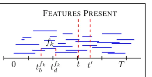
4.1. Dependent Beta Process Construction
The BDFP process can be constructed using a nonho-mogenous Poisson process Π. Consider the L´evy mea-sureν(dωdxdtbdtω)on a product space[0,1]⊗X⊗R⊗
[0,∞). A sample corresponds to set of points Π = {ωk, xk, tkb, t
k
ω}kwhere the range ofkis countably infinite.
Each atom corresponds to a feature and is associated with a weight ωk ∈ [0,1], a locationxk, a birth timetkb ∈ R
and a life-spantk
ω ∈[0,∞)(Figure1). The L´evy measure
x
tb
ω
–1
Figure 1.Cartoon for the dependent Beta process construction of
the BDFP: a realisation of a Poisson processΠover the product
space[0,1]⊗X⊗R⊗[0,∞)is drawn. Thetωdimension over
the space[0,∞)is omitted in the axis representation. However,
eachtωcorresponding to each point (feature) is drawn as ablue
line of lengthtωstarting at the associated birth time point.
corresponds to a Beta process on the combined spaceΘ =
X⊗R⊗[0,∞)withρ(dω) =αω−1(1−ω)α−1andbase
measureµ(dθ) =µ(dxdtbdtw). Settingg(dtb) = dtband
β(dtω) =Dexp−Dtωdtω, the base measure isµ(dθ) =
µ0(dx)g(dtb)β(dtω) =µ0(dx)dtbDexp−Dtωdtω, where
Dis the death rate. The constant measureg(dtb)over the
real lineRis infinite butσ-finite, that is the total measure
g(R) = ∞, but there is a measurable partition(Ek)ofR
with eachg(Ek)<∞. Sinceν(dωdθ)integrates to
infin-ity but satisfiesR[0,1]RΘ(1∧ |ω|)ν(dωdθ)<∞, a count-ably infinite number of i.i.d. random points{(ωk,θk)}∞k=1 are obtained from the Poisson process andP∞
k=1ωkis
fi-nite with probability one. A Beta process is a completely random measure (Kingman,1967) and, as such, a sample can be expressed as B = P∞
k=1ωkδθk|α, µ ∼ BP(αµ),
where the atoms θk = {xk, tkb, t k
ω} ∈ Θ and weights
ωk ∈[0,1].
Having drawn a sampleBwe can construct the feature al-locations over an index spaceRas follows:
B= ∞ X k=1 ωkδθk |α, µ∼BP(αµ) Sn:= ∞ X k=1 bnkδθ |B ∼BeP(ωk) Znk(t) =SnkI(tkb < t < t k b+t k ω) (8)
withbnk|ωk ∼Bernoulli(ωk)andn= 1, . . . , N. The
bi-nary matrixSof dimensionN×K, is afeature potential matrix. Each binary elementSnkindicates whether object
npossesses featurefk. Sis a global variable and doesn’t
depend on timet. At any timet, the feature allocation ma-trixZ(t)is a deterministic function of the current features present att, that is{fk :tkb < t < t
k b +t
k
w, k= 1, . . . ,∞}
and the feature potential matrix S, i.e. Znk(t) = 1iff
Snk= 1andtkb < t < tkb +tkω.
The resulting feature allocation process(zn(t))Tis
equiva-lent to the following: every time a new featurefkis created,
each objectnjoins with probabilityωk, i.e. znk(tkb)|ωk ∼
Bernoulli(ωk). Ifznk(tkb) = 1, objectnwill possess
fea-turefk untiltkb +t k
ω. Repeat this process for all objects.
Proposition 2. TheBDFPis exchangeable and the Beta processBP(αµ)onX⊗R⊗[0,∞)describes its underlying
mixing measure.
Proof. Consider a sequence of variables (zn(t))T with
n= 1,2, . . . , Nsuch that each(zn(t))Tis the feature
allo-cation evolution of objectnover the index spaceT. These
variables are not independent since each(zn(t))Tdepends
on theZ|[n−1](t) = (z1:(n−1)(t))T. However, given a
sam-ple from theB ∼BP(αµ)described in Section4.1, each variable(zn(t))T becomes conditionally independent and
the following holds
P((z1(t))T,(z2(t))T, . . . ,(zN(t))T) = Z N Y n=1 P((zn(t))T|B)φ(dB) (9) whereφ= BP(αµ).
Equation (9) is the de Finetti representation of theBDFP and as such the BDFP is exchangeable and the BP on Θ = X⊗R⊗[0,∞)is its underlying mixing measure.
Restricting our focus on each indext, the overall Beta pro-cessBP(αµ)onX⊗R⊗[0,∞)results in a set of
depen-dentrandom measures overX, oneBtfor eacht∈T, such
that eachBtis marginally a Beta process. Consider a fixed
time pointt ∈Tand the space[0,1]⊗X(the red vertical
plane in Figure1). The point process on this plane (where blue lines intersect the plane) corresponds to features alive at timet, i.e. t ∈[tb, tb+tω]. The L´evy measure on this
plane, is calculated by projecting the overall L´evy measure onto the plane,
νt(dωdx) = Z ∞ 0 Z t t−tω ν(dωdxdtbdtω) =αω−1(1−ω)α−1µ0(dx) D (10)
whereνtis a measure over[0,1]⊗Xfor a specifict ∈T.
More specifically, it is the L´evy measure of a Beta process onXwithρ(dω) = αω−1(1−ω)α−1 and base measure
µt(dx) = µ0D(dx). Thus we have that marginally
Bt|α, µt∼BP(αµt),∀t∈T. (11)
The restricted and projected measure at any indext∈T
de-fines a Beta process. Two draws,BtandBs, witht, s∈T,
will be dependent with the amount of dependence decreas-ing as|s−t|increases.
Proposition 3. The dependent Beta process construction presented hasIBPmarginals at anyt.
Proof. At anyt ∈T,Bt|α, µt∼BP(αµt). It is
straight-forward to see that, marginally, the feature allocation ma-trix Zt obtained using the generative process in
Equa-tion(8)is equivalent toZt|Bt ∼ BeP(Bt)and therefore
Zt∼IBP(α), ∀t∈T.
Corollary 1. At anyt ∈ T, the feature allocation matrix
Ztcan be generated by the following generative model as
K→ ∞: ωk|α∼Beta R K , Znk|ωk∼Bernoulli(ωk) (12) fork= 1, . . . , Kandn= 1, . . . , N
The proof of the corollary in included in the supplementary material. Note that the above is true only marginally, i.e. at timet∈Tand it doesn’t generste dependence structure
betweenZt’s.
We underline the dependence ofZsandZtwhen|s−t| →
0, ∀s, t ∈ T. The closer s, t are, the more the atoms
(features)Bs andBtshare. If we independently sampled
Zs|Bs ∼ BeP(Bs) andZt|Bt ∼ BeP(Bt) thenZs, Zt
would be dependent, but not equal, even as|s−t| → 0. However, in the BDFP the presence of the same features re-sults in thesame(not just similar) allocation as|s−t| →0. In both cases, the marginal distribution of the feature al-location matrix at any t ∈ T is Zt|Bt ∼ BeP(Bt) and
Zt|α∼IBP(α). The BDFP results in a continuous
evolu-tion of theZ(t)overT: formallyZt d
→Zsast→s.
This construction of the BDFP resembles the spatial nor-malised Gamma process (SNΓP) by (Rao & Teh, 2009). The main difference lies in the marginal distribution; the SNΓP admits DP marginals as opposed to the Beta process marginals of the dependent Beta process as shown in Equa-tion (11).
Proposition 4. The feature allocation process described by Equation(8)withB∼BP(αµ), has the same birth and death rates as theBDFprocess.
5. Finite Model
For the BDFP, the inference simplifies considerably if we consider a finite approximation which gives the count-ably infinite model in the limit. Consider the space
S = [0,1]⊗X⊗[0, T]⊗[0,∞), where we restrict the
space of tb to be [0, T] instead of the whole real line R. This accounts for typical applications of the model
where we observe data at distinct times over a finite time range. Consider the L´evy measure ν(dωdxdtbdtω)
on the space S. Then, under the dependent Beta
pro-cess representation (see section 4.1), the expected num-ber of atoms present in S is RSν(dωdxdtbdtω) =
R1 0 ρ(dω) R Xµ0(dx) RT 0 g(dtb) R∞ 0 β(dtω) = KT, where fk tfk b t fk d FEATURESPRESENT t t0 0 T
Figure 2.Cartoon for the Beta event construction of the BDFP: A Poisson(KT) number of features are uniformly distributed
across the time range[0, T](bluelines). Each feature is assigned
a weight sampled fromBeta(R
K,1). The leftmost point of each
line corresponds to the time of birth of that feature, while the length of each line indicates the life span of each feature
sam-pled fromExponential(D). To sample feature allocations from
the process, we consider random time points across time, e.g.t, t0
and draw imaginaryredlines. The feature allocation matrix att
involves the features that are crossing the red line att. The
mem-bership of the objectsn= 1, . . . , Nto those features is defined
by the values of the corresponding elemnts in the potential matrix
S.
K → ∞sinceR01ρ(dω) = ∞. By considering finiteK
we allow inference on a finite model which approximates the infinite case with increasing fidelity asK→ ∞. The process is depicted in Figure2and the infinite case can be derived as the limitK→ ∞of the following:
• Consider a time range[0, T]and a set of featuresF, such that|F | ∼Poisson(KT). Assign to each feature
fk ∈ F, k = 1, . . .|F |a weightω, such thatωk ∼
Beta KR,1
andΩ= [ω1, ω2. . . ω|F |].
• Associate each featurefk ∈ F, k = 1, . . .|F |with
a birth time tk b uniformly sampled in [0, T]; t k b ∼ U(0, T)andtb= [t1b. . . t |F | b ].
• For each fk ∈ F, sample its life span tkw ∼
Exponential(D), whereDis the death rate. Define the time of death tkd as tkd = tkb +tkw and tw =
[t1
w. . . t
|F | w ].
We call the sequence of the above stepsBeta Event Pro-cess (BEP). Putting everything together, generate a sample
B={F,Ω,tb,tw} ∼BEP(α, R, K, T)as follows: |F | ∼Poisson(KT) ωk ∼Beta R K,1 , tkb ∼ U(0, T), tkω∼Exponential(D) (13)
for k = 1, . . . ,|F |. Having drawn a sampleB from the
BEP, we can construct the feature allocations over time as follows Snk|ωk∼Bernoulli(ωk) Znk(t) =SnkI(tkb < t < t k b+t k ω) (14)
wheren= 1, . . . , N. The feature potential matrix (as de-fined in section4.1) has nowN × |F |dimensions. More-over, each Z(t) for t ∈ T is a matrix of dimensions
N ×F(t)andF(t) ≤ |F |. Figure3(a) show the graphi-cal model for the BEP.
R ω S tw Zt tb Yt A σ α t (a) R ω S tw
Z
t tb Yt Wt s α t (b)Figure 3.Graphical representation of the BEP for a time pointt and for (a) a linear-Gaussian likelihood and (b) a sigmoid
likeli-hood. The time seriesZandYare represented as single nodes
indexed by the time locationt. The birth and life span times of
the totalKT features are depicted using vector notationtband
tw. The black (Zt) and grey (Yt) nodes indicate deterministic
and observed parameters respectively.
Proposition 5. In the finite model, the expected number of features present at any t ∈ Tis E[Nf] = KD and for
D= Rα we haveE[Nf] = KαR .
Hyperpriors. We put gamma priors onαandR.
Likelihood models. We consider two different likelihood models: linear-Gaussianfor real data andlogisticfor bi-nary network data.
For the linear-Gaussian likelihood model, consider a se-quence of observations{Yt∈ Y :t= 1, . . . , L}generated
as
Yt=ZtA+t (15)
whereYtis aN×M observation matrix at each timet=
1, . . . , L,Ais a factor loading matrix of dimension|F | ×
Mshared across time andt∼ N 0, σ2
is Gaussian white noise. We choose a Gaussian prior over A, i.eAf m ∼
N(0,1).
In the case of dynamic binary network data we extend the latent feature relational model (LFRM) proposed by (Miller et al.,2009). LetYt be theN ×N binary matrix
that contains links, i.e. ytij =Yt(i, j) = 1iff we observe
a link from entityito entityjat timet. We assume that the matricesYtare symmetric and ignore diagonal elements
(self-links). The probability of a link from one entity to an-other is determined by the combined effect of all pairwise feature interactions. LetWt be a |F | × |F |real-valued
weight matrix whereWt(k, k0) is the weight that affects
the probability of there being a link from entityito entity
jif entityihas featurekon, i.e. Ztik =Zt(i, k) = 1and
entityj has featurek0on, i.e. Ztjk0 =Zt(j, k0) = 1. The links are independent conditioned onZtandWt, and only
the features that are on for the entitiesiandjat timet in-fluence the probability of a link between those entities at that time (see Figure3(b)). Formally,
P(ytij= 1|Zt,Wt) =σ X kl ZtikZtjlWtkl+s (16)
fork, l = 1, . . . ,|F |, wheresis a bias term andσ(x) =
(1 +e−x)−1 is the sigmoid function. For completeness, we assume the priors wt(k, l) ∼ N µw, σ2w
and s ∼ N µs, σs2 . 5.1. Inference
As with many other Bayesian models, exact inference is intractable so we employ Markov Chain Monte Carlo (MCMC) for posterior inference over the latent variables of the finite model. A detailed description is provided in the supplementary material.
6. Experiments
We experimentally evaluate the BEP model on real-world genomics and social network data. To evaluate the model fit, we compared the BEP model to independent models at each time point.
6.1. Circadian Rhythm Dataset
Here we used a subset of the gene expression data from Piechota et al.(2010), includingN = 500genes inD = 4 different conditions (exposure to different drugs) overL= 24time intervals. The measurements indicate how active a gene is at different times. We created7train-test splits holding out 20% of the data, and ran700 MCMC itera-tions. We see that in terms of predictive performance the BEP outperforms independent IBP models (Table1). The genes belonging to each factor show enrichment for differ-ent known biological pathways (Figure4). Of particular note are the tryptophan metabolism genes enriched in fac-tor 2, given tryptophan’s suspected effects on drowsiness;
the vasopressin regulated water reabsorption, given this hormone’s known circadian regulation (Earnest & Sladek, 1986; Yamaguchi et al.,2013); and the regulation of in-sulin producing beta cells, another hormone with circadian variation (Shi et al.,2013).
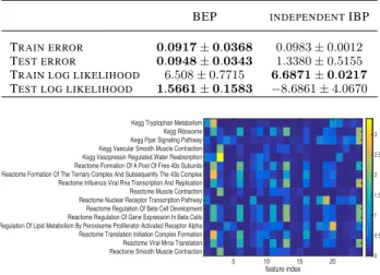
Table 1. Circadian dataset results using 20% held out data, a
trun-cation level ofK= 10,|F |= 24,700iterations and a burnin of
500. Results are the average over 7 MCMC chains.
BEP INDEPENDENTIBP
TRAIN ERROR 0.0917±0.0368 0.0983±0.0012 TEST ERROR 0.0948±0.0343 1.3380±0.5155 TRAIN LOG LIKELIHOOD 6.508±0.7715 6.6871±0.0217
TEST LOG LIKELIHOOD 1.5661±0.1583 −8.6861±4.0670
feature index
5 10 15 20 Kegg Tryptophan Metabolism
Kegg Ribosome Kegg Ppar Signaling Pathway Kegg Vascular Smooth Muscle Contraction Kegg Vasopressin Regulated Water Reabsorption Reactome Formation Of A Pool Of Free 40s Subunits Reactome Formation Of The Ternary Complex And Subsequently The 43s Complex Reactome Influenza Viral Rna Transcription And Replication Reactome Muscle Contraction Reactome Nuclear Receptor Transcription Pathway Reactome Regulation Of Beta Cell Development Reactome Regulation Of Gene Expression In Beta Cells Reactome Regulation Of Lipid Metabolism By Peroxisome Proliferator Activated Receptor Alpha Reactome Translation Initiation Complex Formation Reactome Viral Mrna Translation Reactome Smooth Muscle Contraction
0 0.5 1 1.5 2 2.5 3
Figure 4.Circadian dataset: many of the features uncovered show enrichment in known biological pathways from Reactome and
KEGG. Values here are−log10pfrom a hypergeometric test for
enrichment of the genes in each factor against the 500 background genes.
6.2. ChIP-seq Epigenetic Marks
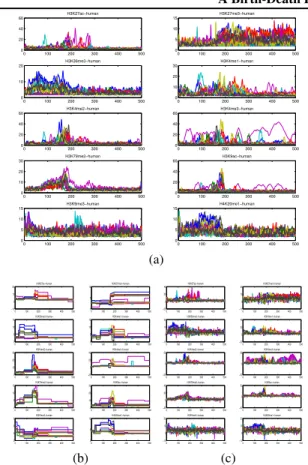
For this experiment we used ChIP-seq (chromatin immuno-precipitation sequencing) data downloaded from the EN-CODE project (Consortium, 2007), representing histone modifications and transcription factor binding in human neural crest cell lines (see (Park,2009) for a nice review). The observations involve counts associated withN = 14 (human) cell lines andD = 10proteins. The counts indi-cate what proteins, with what chemical modifications, are bound to DNA along the genome. The measurements are stored in N ×D matrix of countsYt: for each cell line,
how many reads for each of the 10 proteins mapped to bint
(100base pair (bp) region of the genome).t = 1, . . . ,500 bins were considered at the start of chromosome 1 (50K bp in total). In Figure5(a) each subfigure corresponds to one of the10proteins and in each subfigure the counts for the N = 14 cell lines are plotted over the genome sec-tion of length 50Kbp. Before inference, the raw counts were square-root transformed (a standard variance stabi-lizing transform for Poisson data) to make the Gaussian likelihood appropriate. We ran7 different held-out tests, holding out a different20%of the data each time. Results, using700MCMC iterations, are presented in Table2. The
BEP outperforms the independent IBP model in both test likelihood and error with a statistically significant differ-ence. The independent IBP appears to have better results in train error and likelihood, again suggesting overfitting. Comparing the plots of the true measurements to the learnt ones by the BEP and independent IBP model in Figure5 we see that both models successfully reproduce the data but the BEP reconstructions provide a cleaned up picture of the meaningful signal.
The features found by the model in the different genome locations correspond to different states associated with the specific genome location. Genes and regulatory DNA ele-ments such as enhancers, silencers and insulators are em-bedded in genomes. These genomic elements on the DNA have footprints for the transacting proteins involved in scription, either for the positioning or regulation of the tran-scriptional machinery. For instance, promoters are regions of DNA which recruit proteins required to initiate transcrip-tion of a particular gene and located near the transcriptranscrip-tion start sites. Enhancers are regions of DNA that can be bound by proteins which activate transcription of a distal gene. So a cell line, at specific genome location (recall that here each location corresponds to 100 base pairs), will have un-derlying feature membership (some promoters and some enhancer for example) that determines whether particular protein are found there using ChIP-seq.
Genomic annotations, from ChromHMM (Ernst et al., 2011), are shown in Figure8in the supplementary docu-ment for the region we model. Different levels of the marks in these different regions are much easier to see in the re-constructed signal using BEP in Figure5(b).
Table 2.Quantitative results for the ChIP-seq dataset . 20% held
out data, a truncation level ofK = 3,|F | = 21,700iterations
and a burnin of500. Results are the average over 7 held out sets.
BEP INDEPENDENTIBP
TRAIN ERROR 0.4459±0.0229 0.032±0.0089
TEST ERROR 0.4574±0.018 0.7746±0.013
TRAIN LOG LIKELIHOOD −12.4979±0.1439 −0.5916±0.0979
TEST LOG LIKELIHOOD −3.1666±0.0318 −175.7968±4.49
7. van de Bunt’s Dataset
In van de Bunt et al.(1999), 32 university freshman stu-dents in a given discipline at a Dutch university were sur-veyed at seven time points about who in their class they considered as friends. Initially, i.e.t1, most of the students were unknown to each other. The first four time points are three weeks apart, whereas the last three time points are six weeks apart as showin in Figure11in the supplementary matrial. We symmetrise the matrix by assuming friendship if either individual reported it. We test the performance of BEP using the sigmoid likelihood model as in Equation
0 100 200 300 400 500 0 20 40 60 0 100 200 300 400 500 0 5 10 15 0 100 200 300 400 500 0 10 20 H3K36me3−human 0 100 200 300 400 500 0 10 20 30 H3K4me1−human 0 100 200 300 400 500 0 20 40 60 H3K4me2−human 0 100 200 300 400 500 0 20 40 60 H3K4me3−human 0 100 200 300 400 500 0 10 20 30 H3K79me2−human 0 100 200 300 400 500 0 20 40 60 H3K9ac−human 0 100 200 300 400 500 0 5 10 15 H3K9me3−human 0 100 200 300 400 500 0 5 10 15 H4K20me1−human (a) 0 100 200 300 400 500 −10 0 10 20 H3K27ac−human 0 100 200 300 400 500 0 5 10 H3K27me3−human 0 100 200 300 400 500 0 5 10 15 H3K36me3−human 0 100 200 300 400 500 0 5 10 15 H3K4me1−human 0 100 200 300 400 500 0 10 20 30 H3K4me2−human 0 100 200 300 400 500 −20 0 20 40 H3K4me3−human 0 100 200 300 400 500 0 5 10 15 H3K79me2−human 0 100 200 300 400 500 0 10 20 30 H3K9ac−human 0 100 200 300 400 500 2 4 6 8 H3K9me3−human 0 100 200 300 400 500 0 5 10 H4K20me1−human (b) 0 100 200 300 400 500 −20 0 20 40 H3K27ac−human 0 100 200 300 400 500 −10 0 10 20 H3K27me3−human 0 100 200 300 400 500 −10 0 10 20 H3K36me3−human 0 100 200 300 400 500 −20 0 20 40 H3K4me1−human 0 100 200 300 400 500 −50 0 50 H3K4me2−human 0 100 200 300 400 500 −50 0 50 H3K4me3−human 0 100 200 300 400 500 −20 0 20 40 H3K79me2−human 0 100 200 300 400 500 −50 0 50 H3K9ac−human 0 100 200 300 400 500 −10 0 10 20 H3K9me3−human 0 100 200 300 400 500 −10 0 10 20 H4K20me1−human (c)
Figure 5.ChIP-seq data: The observed (a) and reconstructed ob-servations (b), (c). The BEP reconstructions smooth out the noise making the meaning signal much easier to visualize. In both mod-els, the noise signal was removed from the reconstructions.
(16) by holding out10%of all links across all time points. We ran each model for 1000MCMC iterations. The re-sults are shown in Table3. The independent network LFR models outperform BEP in the train setting and the test er-ror while BEP outperforms in the test likelihood. How-ever, here the results are comparable. Looking at Figure 6, both models provide the same picture of the allocation. It is possible the stationary assumption hurts the BEP: in the VDB dataset the number of links almost exclusively in-creases over time.
Table 3.van de Bunt’s dataset results using 10% held out data, a
truncation level ofK= 4,|F |= 20,1000iterations and a burnin
of200. Results are the average over 7 MCMC chains.
BEP INDEPENDENTLFRM
TRAIN ERROR 1.7009±0.0850 1.3413±0.1147 TEST ERROR 1.9107±0.1321 1.7891±0.1131 TRAIN LOG LIKELIHOOD −1044.4943±41.6363 −839.4544±56.9877 TEST LOG LIKELIHOOD −345.7038±49.9882 −438.5848±74.6396
2 4 6 8101214161820 5 10 15 20 25 30 2 4 6 8101214161820 5 10 15 20 25 30 2 4 6 8101214161820 5 10 15 20 25 30 2 4 6 8101214161820 5 10 15 20 25 30 2 4 6 8101214161820 5 10 15 20 25 30 2 4 6 8101214161820 5 10 15 20 25 30 2 4 6 8101214161820 5 10 15 20 25 30 0.5 1 1.5 2 2.5 5 10 15 20 25 30 1 2 3 4 5 6 7 8 910 5 10 15 20 25 30 0.5 1 1.5 2 2.5 3 3.5 5 10 15 20 25 30 1 2 3 4 5 6 7 8 5 10 15 20 25 30 1 2 3 4 5 6 5 10 15 20 25 30 0.5 1 1.5 2 2.5 3 3.5 5 10 15 20 25 30 0.5 1 1.5 2 2.5 3 3.5 4 4.5 5 10 15 20 25 30
Figure 6.Inferred feature allocation matrices for the seven time points (from left to right) in the van De Bunt friendship dataset.
First two rows: Feature allocation matrices inferred by BEP.
Last two rows:Feature allocation matrices inferred by indepen-dent LFRM.
8. Discussion
Many modern machine learning and statistics tasks involve multidimensional data positioned along some linear covari-ate: we have shown functional genomics data where the co-variate is position in the genome, and network data where links change over time. To model such data we need pri-ors that utilize the dependencies through time, while han-dling high dimensionality. The BDFP is an expressive new Bayesian non-parametric prior that fulfills these criteria. It outputs time-evolving feature allocations, which can then be effectively used to model high-dimensional time-series data. Since the number of latent features is unbounded, like other Bayesian non-parametric methods, the model can adapt its complexity to the data. While the combi-natorial BDFP may seem like a complex object to handle computationally, our theoretical results showing that the de Finetti measure underlying the BDFP is a specific beta pro-cess, which can be well approximated by a finiteKmodel, the BEP. Our experimental results, compared to indepen-dent feature allocations, provides evidence that effectively modeling dependency in the feature allocation through the birth-death mechanism is appropriate for a wide range of statistical applications. Moreover, the BEP provides an in-terpretable structure using parameters not found, to the best of our knowledge, in existing models, i.e. birth and death rate of features. We are interested in scaling inference un-der the BEP to larger datasets, for example using (stochas-tic) variational inference methods that have been successful for the IBP (Doshi et al.,2009).
Acknowledgements Konstantina’s research leading to these results has received funding from the European Research Coun-cil under the European Union’s Seventh Framework Programme (FP7/2007-2013) ERC grant agreement no. 617411.
References
Aldous, D J. Exchangeability and related topics. InEcole d’Ete de
Probabilities de Saint-Flour, volume XIII, pp. 1–198. Springer,
1983.
Consortium, The ENCODE Project. Identification and analysis of functional elements in 1% of the human genome by the
EN-CODE pilot project.Nature, 447(7146):799–816, 06 2007.
de Finetti, B.Funzione Caratteristica Di un Fenomeno Aleatorio,
pp. 251–299. 6. Memorie. Academia Nazionale del Linceo, 1931.
Doshi, F., Miller, K. T., Van Gael, J., and Teh, Y. W. Variational
inference for the Indian buffet process. InProceedings of the
International Conference on Artificial Intelligence and
Statis-tics, volume 12, 2009.
Earnest, David J and Sladek, Celia D. Circadian rhythms of vaso-pressin release from individual rat suprachiasmatic explants in
vitro.Brain research, 382(1):129–133, 1986.
Ernst, Jason, Kheradpour, Pouya, Mikkelsen, Tarjei S, Shoresh, Noam, Ward, Lucas D, Epstein, Charles B, Zhang, Xiaolan, Wang, Li, Issner, Robbyn, Coyne, Michael, et al. Mapping and analysis of chromatin state dynamics in nine human cell types.
Nature, 473(7345):43–49, 2011.
Ghahramani, Zoubin and Jordan, Michael. Factorial hidden
markov models.Machine Learning, 29(2-3):245–273, 1997.
Griffiths, Thomas L. and Ghahramani, Zoubin. Infinite latent
fea-ture models and the indian buffet process. InIn NIPS, pp. 475–
482. MIT Press, 2005.
Griffiths, Thomas L. and Ghahramani, Zoubin. The indian
buf-fet process: An introduction and review. Journal of Machine
Learning Research, 12:1185–1224, July 2011.
Hjort, N. L. Nonparametric Bayes estimators based on Beta
pro-cesses in models for life history data. Annals of Statistics, 18:
1259–1294, 1990.
Kingman, J.F.C. The coalescent. Stochastic Processes and their
Applications, 13(3):235 – 248, 1982.
Kingman, John F. C. Completely Random Measures.Pacific
Jour-nal of Mathematics, 21(1):59–78, 1967.
Miller, Kurt, Griffiths, Thomas, and Jordan, Michael.
Nonpara-metric latent feature models for link prediction. InAdvances in
Neural Information Processing Systems 22, 2009.
Neal, Radford M. Density Modeling and Clustering Using
Dirich-let Diffusion Trees. In Bayesian Statistics 7, pp. 619–629,
2003.
Palla, Konstantina, Knowles, David A., and Ghahramani, Zoubin. A dependent partition-valued process for multitask clustering and time evolving network modelling, 2013.
Park, Peter J. Chip–seq: advantages and challenges of a maturing
technology.Nature Reviews Genetics, 10(10):669–680, 2009.
Piechota, Marcin, Korostynski, Michal, Solecki, Wojciech, Gieryk, Agnieszka, Slezak, Michal, Bilecki, Wiktor, Zi-olkowska, Barbara, Kostrzewa, Elzbieta, Cymerman, Iwona, Swiech, Lukasz, et al. The dissection of transcriptional mod-ules regulated by various drugs of abuse in the mouse striatum.
Genome Biology, 11(5):R48, 2010.
Rao, Vinayak and Teh, Yee Whye. Spatial normalized gamma processes. 2009.
Rasmussen, Carl Edward and Williams, Christopher K I.
Gaus-sian processes for machine learning. MIT Press, 2006.
Shi, Shu-qun, Ansari, Tasneem S, McGuinness, Owen P, Wasser-man, David H, and Johnson, Carl Hirschie. Circadian
disrup-tion leads to insulin resistance and obesity. Current Biology,
23(5):372–381, 2013.
Teh, Y. W., Elliott, L. T., and Blundell, C. Bayesian nonpara-metric modelling of genetic variations using fragmentation-coagulation processes. Submitted, 2013.
Thibaux, Romain and Jordan, Michael I. Hierarchical beta
pro-cesses and the indian buffet process. InProceedings of the
Eleventh International Conference on Artificial Intelligence
and Statistics (AISTATS), volume 2, pp. 564–571, 2007.
van de Bunt, Gerhard G, Van Duijn, Marijtje AJ, and Snijders, Tom AB. Friendship networks through time: An actor-oriented
dynamic statistical network model. Computational &
Mathe-matical Organization Theory, 5:167–192, 1999.
Van Gael, J., Teh, Y. W., and Ghahramani, Z. The infinite
facto-rial hidden Markov model. InAdvances in Neural Information
Processing Systems, volume 21, 2009.
Williamson, Sinead, Orbanz, Peter, and Ghahramani, Zoubin.
De-pendent Indian buffet processes. InProceedings of the
Thir-teenth International Workshop on Artificial Intelligence and
Statistics, AISTATS, 2010.
Yamaguchi, Yoshiaki, Suzuki, Toru, Mizoro, Yasutaka, Kori, Hi-roshi, Okada, Kazuki, Chen, Yulin, Fustin, Jean-Michel, Ya-mazaki, Fumiyoshi, Mizuguchi, Naoki, Zhang, Jing, et al. Mice genetically deficient in vasopressin v1a and v1b
![Figure 1. Cartoon for the dependent Beta process construction of the BDFP: a realisation of a Poisson process Π over the product space [0, 1] ⊗ X ⊗ R ⊗ [0, ∞) is drawn](https://thumb-us.123doks.com/thumbv2/123dok_us/1989409.2795490/4.918.82.423.93.312/figure-cartoon-dependent-process-construction-realisation-poisson-process.webp)