Model confidence sets and forecast combination: an application to age-specific mortality

City, University of London Institutional Repository

Citation

: Haberman, S. ORCID: 0000-0003-2269-9759 and Shang, H.L. (2018). Model

This is the accepted version of the paper.

This version of the publication may differ from the final published

version.

Permanent repository link:

Link to published version

:

Copyright and reuse:

City Research Online aims to make research

outputs of City, University of London available to a wider audience.

Copyright and Moral Rights remain with the author(s) and/or copyright

holders. URLs from City Research Online may be freely distributed and

linked to.

City Research Online: http://openaccess.city.ac.uk/ [email protected]

Model confidence sets and forecast combination:

An application to age-specific mortality

September 28, 2018

Abstract

Background: Model averaging combines forecasts obtained from a range of models, and it often produces more accurate forecasts than a forecast from a single model.

Objective: The crucial part of forecast accuracy improvement in using the model averaging lies in the determination of optimal weights from a finite sample. If the weights are selected sub-optimally, this can affect the accuracy of the model-averaged forecasts. Instead of choosing the optimal weights, we consider trimming a set of models before equally averaging forecasts from the selected superior models.Motivated byHansen et al.(2011), we apply and evaluate the model confidence set procedure when combining mortality forecasts.

Data & Methods: The proposed model averaging procedure is motivated bySamuels and Sekkel(2017) based on the concept of model confidence sets as proposed by Hansen et al.

(2011) that incorporates the statistical significance of the forecasting performance. As the model confidence level increases, the set of superior models generally decreases. The proposed model averaging procedure is demonstrated via national and sub-national Japanese mortality for retirement ages between 60 and 100+.

Results: Illustrated by national and sub-national Japanese mortality for ages between 60 and 100+, the proposed model-average procedure gives the smallest interval forecast errors, especially for males.

Conclusion: We find that robust out-of-sample point and interval forecasts may be obtained from the trimming method. By robust, we mean robustness against model misspecification. Keywords: Equal predictability test; Japanese Human Mortality Database; Mean interval score; Model averaging; Root mean square forecast error.

1

Introduction

Because of declining mortality rates in mainly developed countries, the improvement in human survival probability contributes significantly to an aging population. As a consequence, pension funds and insurance companies face longevity risk. The longevity risk is a potential risk attached to the increasing life expectancy of policyholders, which can eventually result in a higher payout ratio than expected (Crawford et al.,2008). The concerns about longevity risk have led to a surge in interest among pension funds and insurance companies in accurately modeling and forecasting age-specific mortality rates (or death counts or survival probabilities). Any improvement in the forecast accuracy of mortality rates will be beneficial for determining the allocation of current and future resources at the national and sub-national levels (see, e.g.,Koissia,2006;Denuit et al.,2007;

Hanewald et al.,2011).

Many different models for forecasting age-specific mortality rates have been proposed in the literature (seeBooth,2006;Booth and Tickle,2008;Currie et al.,2004;Girosi and King,2008;Shang et al.,2011;Tickle and Booth,2014, for reviews). Of these, a significant milestone in demographic modeling and forecasting was the work byLee and Carter(1992). They implemented a principal component method to model age-specific mortality and extracted a single time-varying index representing the trend in the level of mortality rates, from which the forecasts are obtained by a random walk with drift. While the Lee-Carter method is simple and robust in situations where age-specific log mortality rates have linear trends (Booth,2006), it has the limitation of attempting to capture the patterns of mortality rates using only one principal component and its associated scores. To rectify this deficiency, the Lee-Carter method has been extended and modified. For example, from a discrete data matrix perspective,Booth et al.(2002),Renshaw and Haberman

(2003a) andCairns et al.(2006,2009) proposed the use of more than one component in the Lee-Carter method to model age-specific mortality rates;Renshaw and Haberman(2006) proposed an age-period-cohort extension to the Lee-Carter model under a Poisson error structure, whilePlat

(2009b) extended this model by incorporating the dependence between ages. Cairns et al.(2006) used a logistic transformation to model the relationship between the death probability and age observed over time, whileCairns et al.(2009) extended this model by incorporating the cohort effect. Girosi and King(2008) andWi´sniowski et al.(2015) considered a Bayesian paradigm for the Lee-Carter model estimation and forecasting. Hatzopoulos and Haberman(2009) followed a Generalized Linear Model approach which leads to models that have a similar structure to the Lee-Carter model but with a generalized error structure.Hunt and Blake(2014) presented a general structural form of mortality models. From a continuous function perspective,Hyndman

and Ullah(2007) proposed a functional data model that utilizes nonparametric smoothing and higher-order principal components, while Shang et al. (2011) and Shang (2016) considered a multilevel functional data model to model mortality rates jointly for multiple populations.

There exist many papers on comparing the forecast accuracy among several mortality forecast-ing methods. However, the most accurate forecastforecast-ing method has been determined based on an aggregate loss function. Instead of identifying the most accurate method,Shang(2012) considered a model averaging approach to combine forecasts from a range of methods, such as the Lee-Carter and functional time series methods. In this paper, we propose a new model averaging approach motivated bySamuels and Sekkel(2017). The proposed model averaging method uses the model confidence set procedure to select a set of superior models and combines the forecasts by assigning equal weights to the set of superior models. In contrast withShang(2012), the problem is centered not on the selection of optimal weights, but on the selection of superior models. In Section6, we compare the forecast accuracy between the existing and proposed model average methods.

With the aim of evaluating and comparing the forecast accuracy of different forecasting meth-ods, forecast competition has a long history. The “M” competition originated fromMakridakis et al.(1979) was the first attempt at a large empirical comparison of forecasting methods. In that “M” competition, there were 1001 time series for which participants were invited to submit their forecasts. Later, the results were published in Makridakis et al. (1982). The “M” competition has progressed slowly over the years, with the most recent M4 competition taken place in 2018. The top-performing teams all combine forecasts from a range of statistical and machine learning methods via some model averaging to improve the point and interval forecast accuracies.

Despite the popularity of model averaging in statistical and forecasting literature (see, e.g.,

Bates and Granger, 1969; Dickinson, 1975; Clemen, 1989), model averaging has not received increasing attention in the demographic literature with the noticeable exceptions ofShang(2012,

2015) in the context of mortality forecasting, Bijak(2011, Chapter 5) in the context of migration forecasting,Abel et al.(2013) andShang et al.(2014) for the overall population growth rate. Shang

(2012) revisited many statistical methods and combined their forecasts based on two weighting schemes, one of which has been adapted for comparison in Section6. Both weighting schemes determine the weights by using either in-sample forecast accuracy or in-sample goodness-of-fit. Because of the finite sample, the weight assigned to the worst model is often small but not zero. In turn, this may lead to inferior forecast accuracy than the one based on Oracle weights. This motivates us to consider an alternative model averaging idea. Instead of assigning weights to the forecasts from all models, we trim out the worse performing models based on a statistical significance test, such as the model confidence set procedure of Hansen et al.(2011) (see also

Samuels and Sekkel,2017).

While most attention has been paid to selecting model combination weights (see, e.g.,Fischer and Harvey, 1999; Genre et al.,2013),Aiolfi et al. (2010) pointed out that there has been little research focusing on which models to include in the model pool. Graefe(2015) asserted that a simple average of the forecasts produced by individual models is a benchmark, and commonly outperforms more complicated weighting schemes that rely on the estimation of theoretically optimal weights. The simple average of the forecasts performs well when the model fits the data poorly; when the sample number per predictor is low and when the predictors are highly correlated (Graefe,2015).

This paper focuses on a statistical significance approach to select the models to be included in the forecast combination. Via the model confidence set procedure ofHansen et al.(2011), we determine a set of statistically superior models, conditional on the model’s in-sample performance for forecasting age-specific mortality rates. By equally averaging the forecasts from the superior models, we evaluate and compare point and interval forecast accuracies, as measured by the root mean square forecast error and mean interval score, respectively.

The outline of this paper is described as follows: From the Japanese national and sub-national age-specific mortality data in Section2, we first visualize the heterogeneity in age-specific mortality rates among 47 prefectures. Then, we revisit some commonly used multivariate and functional time-series extrapolation methods for forecasting age-specific mortality rates in Section3. Using the model confidence set procedure ofHansen et al. (2011) described in Section4, we select a set of superior models based on their point or interval forecast accuracy and demonstrate the robust accuracy of the proposed model averaging method in Section5. In Section6, we present an adaption of an existing model-averaging method where optimal weights are estimated based on in-sample forecast accuracy and assigned to the forecasts from all models. In Section7, we conclude and outline how the methodology presented here can be further extended.

2

Japanese national and sub-national age-specific mortality data

We study the Japanese age-specific mortality rates from 1975 to 2015, obtained from theJapanese Mortality Database(2017). We consider ages from 60 to 99 in single years of age, while the last age group contains all ages at and beyond 100 (abbreviated as 100+). We consider modeling mortality at older ages, as the mortality forecasts are an important input for calculating annuity prices for retirees and the corresponding reserves held by insurance companies and pension funds. Some of the models considered were designed for modeling mortality at older ages, such as the

Cairns-Blake-Dowd models.

We split the Japanese mortality rates by sex and prefecture. We are also interested in the mortality data at the sub-national (i.e., prefecture) level. The mortality forecasts at the prefecture level are more useful than the mortality forecasts at the national level for local policy making and planning.

In the supplement, we have plotted the geographic locations (from North to South) of the 47 prefectures within eight regions of Japan. Also, we present the names of prefecture within each of the eight regions of Japan.Shang and Haberman(2017) andShang and Hyndman(2017) present plots of the ratio of mortality between each prefecture and Japan by age or year.

3

Time-series extrapolation models

We study some time-series extrapolation methods for modeling and forecasting age-specific mortality rates. The models that we have considered are subjective and far from extensive, but they suffice to serve as a test bed for demonstrating the performance of forecast combination. From actuarial science, we consider a family of Renshaw-Haberman (RH) models (see, e.g.,Renshaw and Haberman,2003a,b,2006,2008;Haberman and Renshaw,2008,2009) and a family of Cairns-Blake-Dowd (CBD) models (Cairns et al.,2006). These two models perform well for mortality at higher ages, such as between 60 and 100+. From demography, we consider a family of Lee-Carter (LC) models (see, e.g.,Lee and Carter,1992;Booth et al.,2006;Zhao,2012;Zhao et al.,2013). From statistics, we consider a family of functional time-series models (see, e.g.,Hyndman and Booth,

2008;Hyndman and Shang,2009;Hyndman et al.,2013). For implementation, we use the StMoMo package of Villegas et al.(2018) for the RH and CBD models; we use the demography package ofHyndman(2017) for the LC models for the Gaussian error setting and functional time-series models.

3.1

Notations

Let the random variableDx,t be the number of death counts in a population at agex and year

t. A rectangular data array (dx,t,ex,t) is available for data analysis where dx,t is the observed

number of deaths and ex,t is the corresponding exposure to risk (Hatzopoulos and Haberman, 2009). The force of mortality and central mortality rates are given by µx,t and mx,t = dx,t/ex,t,

respectively. Cross-classification is by individual calendar yeart ∈ [t1,tn](rangen) and by age

x ∈ [x1,xk], either grouped intok(ordered) categories, or by individual year (rangek), in which

Hatzopoulos and Haberman,2009).

3.2

Lee-Carter model under a Gaussian error setting

With the central mortality ratesmx,t, the LC model structure is

mx,t =expαx+β

(1)

x κ(_t1)+εx,t_{, (1)}

lnmx,t =αx+β(x1)κ_t(1)+εx,t

subject to the identification constraints

tn

∑

∑

Note thatαx is the age pattern of the log mortality rates averaged across years; β(x1) is the first

principal component capturing relative change in the log mortality rate at each agex;κ(_t1)is the

first set of principal component scores measuring general level of the log mortality rate at yeart; bilinear termsβ(x1)κ(_t1)incorporating the age-specific period trends (Pitacco et al.,2009, Section 6.2);

andεx,tis the model residual at agexand yeart.

In the demographic forecasting literature, the LC model adjusts κt by refitting to the total

number of deaths (seeLee and Carter,1992). In theLee and Miller’s (2001) method, the adjustment ofκt involves fitting life expectancy at birth in the yeart. In theBooth et al.’s (2006) method, the

adjustment ofκt involves fitting to the age distribution of deaths rather than to the total number of

deaths.

The adjusted principal component scores{κ1, . . . ,κn}are then extrapolated by a random walk

with drift method, from which forecasts are obtained by (1) with the estimated mean functionαx

and principal componentβx. That is,

lnmbx,n+h|n =bαx+βbxbκn+h|n,

where bκn+h|n denotes forecasts of principal component scores obtained from a univariate time

series forecasting method, such as the random walk with drift.

Two sources of uncertainty ought be considered: estimation errors in the parameters of the LC model and forecast errors in the forecast principal component scores. Because of orthogonality between the first principal component and the error term in (1), the overall forecast variance can be approximated by the sum of the two variances (see alsoLee and Carter,1992). Conditioning on the past dataJ = (m₁, . . . ,m_n)and the first principal componentbx, we obtained the overall

forecast variance of ln(mx,n+h), var ln(mx,n+h) J,b_x ≈b2_xu_n+h|n+vx, (2)

whereb2xis the variance of the first principal component, calculated as the square of theβxin (1);

u_n+h|n = var(κn+h|κ1, . . . ,κn) can be obtained from the univariate time-series model; and the

model residual variancevx is estimated by averaging the residual squares{e2_x,1, . . . ,e2x,n}for each

xin (1).

3.3

Renshaw-Haberman model under a Poisson error setting

Renshaw and Haberman(2006) generalizes the LC model structure to include age-period-cohort modeling by formulating the mortality reduction factor as

lnmx,t =αx+β(x1)κ_t(1)+β(x0)γt−x, (3)

where αx is an age function capturing the general shape of mortality by age; a time index κ(_t1)

specifies the mortality trend andβ(x1) modulates its effect across ages; andγt−xdenotes a random

cohort effect as a function of the birth-year(t−x)(see alsoVillegas et al.,2018). To estimate the parameters in (3),Renshaw and Haberman(2006) assume a Poisson distribution of deaths and use a log-link function targeting the force of mortality.

To facilitate the model identifiability, a set of parameter constraints are imposed by setting

∑

∑

∑

∑

3.3.1 Age-period-cohort (APC) model

The APC model studied byClayton and Schifflers(1987a,b) can be derived from theRenshaw and Haberman(2006) model. The APC model corresponds toβ(x1) =β(x0) =1 in (3), that is

lnmx,t =αx+κ(_t1)+γt−x.

To ensure the model identifiability, a set of parameters are constrained by setting

∑

∑

∑

3.4

Cairns-Blake-Dowd (CBD) model

While the LC model is a data-driven method, the CBD model attempts to find factors that may affect age-specific log mortality rates. The former approach is nonparametric, while the latter one is parametric. Note that in the original CBD model, the authors proposed the modeling of age-specific death probabilityqx,t. Here, for the sake of comparison, we use the CBD model to

model and forecast age-specific log mortality rates.Let the pre-specific age-modulating parameters beβ(x1) =1 andβ(x2) = x−x¯, the CBD model can be expressed as

lnmx,t =κ(_t1)+ (x−x¯)κ(_t2), (4)

where ¯x is the average age in the sample range. While κ_t(1) can be viewed as a time-varying

interpret, κ_t(2) can be viewed as a time-varying slope. Cairns et al. (2006) produce mortality

forecasts by projectingκ(_t1) andκ(_t2)jointly using a bivariate random walk with drift.

3.4.1 M7: Quadratic CBD model with cohort effects

Cairns et al.(2009) extend the original CBD model in (4) by adding a cohort effect and a quadratic age effect to form

lnmx,t =κ(_t1)+ (x−x¯)κ_t(2)+ [(x−x¯)2−bσ 2 x]κ (3) t +γt−x, wherebσ 2

x is the average value of(x−x¯)2. To ensure the model identifiability,Cairns et al.(2009)

impose a set of constraints:

tn−x1

∑

∑

∑

In addition to M7 model,Cairns et al.(2009) also consider two simpler predictors given by

lnmx,t =κ_t(1)+ (x−x¯)κ(_t2)+γt−x, (5)

lnmx,t =κ_t(1)+ (x−x¯)κ(_t2)+ (xc −x)γt−x, (6)

wherexc is a constant parameter to be estimated. Equations (5) and (6) are referred to as M6 and

M8, respectively.

3.4.2 Plat model

By combing the features of the LC and CBD models,Plat(2009a) proposed the following model

lnmx,t =αx+κ(_t1)+ (x¯−x)κ_t(2)+ (x¯−x)+κ(_t3)+γt−x. (7)

where(x¯−x)+ =max(x¯−x, 0). To ensure the model identifiability, the following set of parameter constraints have been imposed

∑

∑

∑

∑

∑

∑

In the families of the RH and CBD models,Cairns et al.(2006,2011),Haberman and Renshaw

(2011) andVillegas et al.(2018) assume that the period indexes follow a multivariate random walk with drift. For the cohort index, they assume it follows a univariate autoregressive integrated moving average model.

3.5

The functional time-series models for one population

3.5.1 Functional principal component analysis

Hyndman and Ullah(2007) consider a functional time-series model for forecasting age-specific mortality rate, where age is treated as a continuum. The functional time-series model allows one to smooth the observed data points, in order to reduce or eliminate measurement error. To smooth data,Hyndman and Ullah(2007) suggest the use of a penalized regression spline with monotonic constraints applied to age-specific log mortality rates denoted by lnmt(x) (see Hyndman and Ullah,2007, for detail). Here, we propose to smooth age-specific mortality rates from ages 0 to 100+, and then truncate the smoothed mortality rates from 60 to 100+.

With smoothed age-specific log mortality curves (lnmt(x)), we obtain a mean function denoted

byµ(x). With the de-centered smoothed data, we apply a functional principal component analysis to reduce dimensionality to some functional principal components (i.e,φk(x)) and their associated

scores (βk = (β1,k, . . . ,βn,k)). The functional principal component is constructed by sample

variance of discretized functional data. Conditioning on the observed data and the estimated principal components, the point forecast of future mortality curves can be obtained by forecasting estimated principal component scores via a univariate time-series method. The prediction interval can be constructed similarly to the way of constructing prediction intervals for the Lee-Carter method in Section2.

3.5.2 Robust functional principal component analysis

Because the presence of outliers can seriously affect the performance of modeling and forecasting, it is important to eliminate the effect of outliers where possible. As considered inHyndman and Ullah(2007), the robust functional time-series method calculates the integrated squared error for each year, that is

Z I h lnmt(x)−µ(x)− K

∑

The integrated squared error provides a measure of estimation accuracy for the functional principal component approximation of the functional data. Outliers are those years that have a larger integrated squared error than a critical value calculated from aχ2distribution (seeHyndman and

Ullah,2007, for details). By assigning zero weight to outliers, we can again apply the functional time-series method to model and forecast age-specific mortality rates.

3.6

The functional time-series models for multiple subpopulations

When forecasting age-specific mortality for multiple subpopulations, it is advantageous to use a model that can capture correlation among subpopulations as the covariance of the multiple subpopulations often exhibits cross-correlation. By modeling the cross-correlation, it may improve forecast accuracy. Here, we consider the problem of jointly modeling and forecasting female and male mortality in order to produce coherent forecasts. Note that coherent forecasts can also be achieved by jointly modeling female or male mortality for all 47 prefectures.

3.6.1 Product-ratio method ofHyndman et al.(2013)

InHyndman et al.(2013), they define the square roots of the product and ratio functions of the smoothed mortality rates for female and male data:

pt(x) = q mM_t (x)mF_t(x), rt(x) = q mM_t (x)/mF_t(x).

Instead of modeling female and male mortality data, we model the product and ratio functions. The advantage of this approach is that the product and ratio functions tend to behave roughly independently of each other, provided that the multiple subpopulations have approximately equal variances. On the logarithmic scale, these are sums and differences that are nearly uncorrelated. The functional time-series method in Section3.5can be applied to forecast the product and ratio functions (seeHyndman et al.,2013, fore details).

3.6.2 Multivariate functional time-series method

We consider data where each observation consists ofw ≥2 functions,[lnm(1)(x), . . . , lnm(w)(x)]> ∈

Rw. These multivariate functions are defined over the same domainI (e.g.,Jacques and Preda,

2014;Chiou et al.,2014;Shang and Yang,2017).

We followShang and Yang(2017) and consider the stacking of multiple subpopulations into a long vector of functions, i.e., we stack the discretized data points of each sub-population together for the same year. Then, we perform a multivariate functional principal component analysis to reduce dimensionality and summarize the main mode of information. With the extracted principal components and their scores, a functional time-series method in Section3.5can be applied again.

3.6.3 Multilevel functional time-series method

The multilevel functional data model has a strong resemblance to a two-way functional analysis of variance model studied byMorris et al.(2003);Cuesta-Albertos and Febrero-Bande(2010) and (Zhang,2014, Section 5.4). It is a special case of the general ‘functional mixed model’ proposed in

Morris and Carroll(2006). In the case of two subpopulations, the basic idea is to decompose age-specific log mortality curves among different subpopulations into a sex-age-specific averageµj(x), a

common trend across subpopulationsRt(x), a sex-specific residual trendU_tj(x), and measurement

errorej_t(x)with finite variance(σ2)j(see, e.g.,Hatzopoulos and Haberman,2013;Shang,2016). The common and sex-specific residual trends are modeled by projecting them onto the eigenvectors of covariance operators of the aggregate and population-specific centered stochastic processes, respectively.

4

Model confidence set

The model confidence set procedure proposed byHansen et al.(2011) consists of a sequence of tests permitting the construction of a set of “superior” models, where the null hypothesis of equal predictive ability (EPA) is not rejected at a specified confidence level. The EPA test statistic can be evaluated for any arbitrary loss function, such as the square or absolute loss function.

Let Mbe some subset of original models denoted by M0and letmbe the number of models in

M, and letdρξ,`denote the loss differential between two modelsρandξ, that is

dρξ,` =lρ,`−lξ,`, ρ,ξ =1, . . . ,m, `=1, . . . ,N,

and calculate

dρ·,` =

1

m_ξ

∑

as the loss of modelρrelative to any other modelξat time point`. Letcρξ =E(dρξ)andcρ. =E(dρ.)

be finite and not time dependent. The EPA hypothesis for a set of Mcandidate models can be formulated in two ways:

H0,M : cρξ =0, for all ρ,ξ =1, 2, . . . ,m

HA,M : cρξ 6=0, for some ρ,ξ =1, 2, . . . ,m. (8)

or

H0,M : cρ. =0, for all ρ=1, 2, . . . ,m

Based oncρξ orcρ., we construct two hypothesis tests as follows: tρξ = dρξ q d Var(dρξ) , (10) tρ. = dρ. q d Var(dρ.) , (11)

where dρ. = _m1 ∑ξ∈Mdρξ is the sample loss of the ρth model compared to the averaged loss

across models, and dρξ = _m1 ∑

m

`=1dρξ,` measures the relative sample loss between the ρ

th _and

ξth models. Note that Vard dρ. and dVar dρξ

are the bootstrapped estimates of Vardρ.

and Vardρξ

, respectively. Bernardi and Catania(2014) perform a block bootstrap procedure with 5,000 bootstrap samples by default, where the block length is given by the maximum number of significant parameters obtained by fitting an autoregressive process on all thedρξ terms. For both

hypotheses in (8) and (9), there exist two test statistics:

TR,M = max ρ,ξ∈M t_ρξ , T_max,M =max ρ∈M tρ.,

where tρξ and tρ. are defined in (10) and (11), respectively. WhileTR,M uses the loss differential

between modelsρandξ,Tmax,Muses the aggregated loss differential between modelsρandξ over

ξ. Oftentimes but not always, the models selected on the basis ofTR,M form a subset of the models

selected on the basis ofTmax,M.

The Model Confidence Set (MCS) procedure is a sequential testing procedure, which eliminates the worst model at each step until the hypothesis of equal predictive ability is accepted for all the models belonging to a set of superior models. The selection of the worst model is determined by an elimination rule that is consistent with the test statistic,

eR,M =argmax ρ∈M        sup ξ∈M dρξ r d Vardρξ        , emax,M =argmax ρ∈M dρ. d Vardρ. .

5

Forecast results

5.1

Point forecast evaluation

An expanding window analysis of a time series model is commonly used to assess model and parameter stabilities over time. It assesses the constancy of a model’s parameter by computing parameter estimates and their corresponding forecasts over an expanding window of a fixed size through the sample size (see Zivot and Wang, 2006, Chapter 9 for details). Using the first 21

observations from 1975 to 1995 in the Japanese age-specific mortality rates, we produce one-step-ahead point forecasts. Through an expanding window approach, we re-estimate the parameters in the time series forecasting models using the first 22 observations from 1975 to 1996. Forecasts from the estimated models are then produced for one-step-ahead. We iterate this process by increasing the sample size by one year until reaching the end of the training data period in 2005. This process produces ten one-step-ahead forecasts in the validation data period from 1996 to 2005. We compare these forecasts with the holdout samples to determine the point and interval forecast accuracies. By using the MCS procedure, we identify a superior set of models for averaging. Through the expanding window approach, we evaluate the out-of-sample point and interval forecast accuracies for the testing data from 2006 to 2015.

To evaluate the point forecast accuracy, we use the root mean squared forecast error (RMSFE). The RMSFE measures how close the forecasts are in comparison to the actual values of the variable being forecast. For each series, they can be written as

RMSFEξ = v u u t 1 41 41

∑

whereY_n+ξ(xj)represents the actual holdout sample for thejthage andξthcurve of the forecasting

period, whileYb_n+ξ(x_j)represents the point forecasts for the holdout sample.

5.2

Interval forecast evaluation

In addition to point forecasts, we also evaluate the pointwise interval forecast accuracy using the interval score ofGneiting and Raftery(2007) (see alsoGneiting and Katzfuss,2014). For each year in the forecasting period, the one-step-ahead prediction intervals were calculated at the 100(1−α)%

nominal coverage probability. We consider the common case of symmetric 100(1−α)% prediction interval, with lower and upper bounds that are predictive quantiles atα/2 and 1−α/2, denotes by

b

Yl

n+ξ(xi)andYb

u

n+ξ(xi). As defined byGneiting and Raftery(2007), a scoring rule for thepointwise

interval forecast at time pointxi is

Sα h b Y_nl_+ξ(xi),Yb_nu_+ξ(x_i);Y_n+ξ(xi) i =hYb_nu_+ξ(x_i)−Yb_nl_+ξ(x_i) i +2 α h b Y_nl_+ξ(xi)− Yn+ξ(xi) i 1nYb_n+ξ(xi)<Yn+ξ(xi) o +2 α h Yn+ξ(xi)−Yb_nu_+ξ(x_i) i 1nYn+ξ(xi)>Yb_n+ξ(xi) o ,

whereαdenotes the level of significance, customarilyα =0.2; and1{·}denotes a binary indicator.

The optimal interval score is achieved whenYn+ξ(xi)lies betweenYb_nl₊

ξ(xi)andYb

u

n+ξ(xi), with

We define the mean interval score for different points in a curve and different lengths in the forecasting period as Sα,ξ = 1 41 41

∑

denotes the interval score at the ξth curve of the

fore-casting period.

5.3

Determining a superior set of models

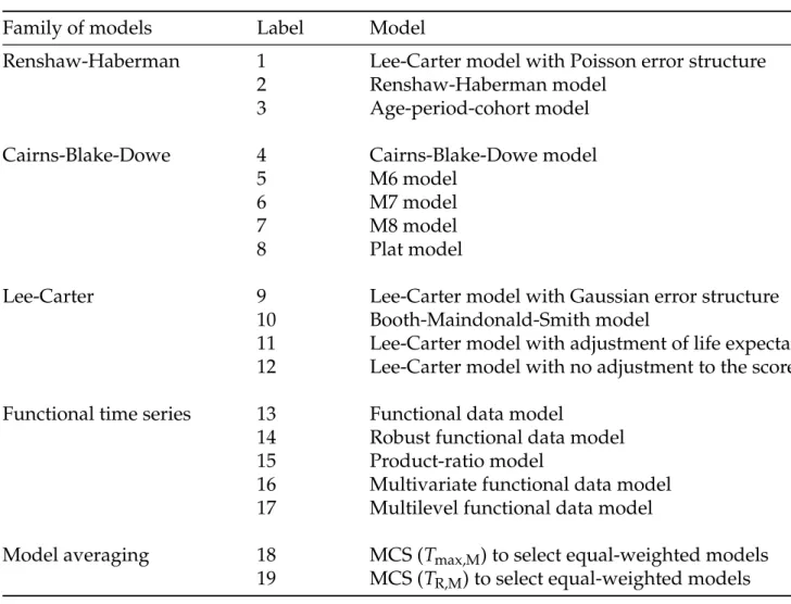
Based on the RMSFE error measure in the training data, we examine statistical significance in point forecast accuracy among the 17 time-series extrapolation methods. The 17 models considered are listed in Table1.

[Table 1 about here.]

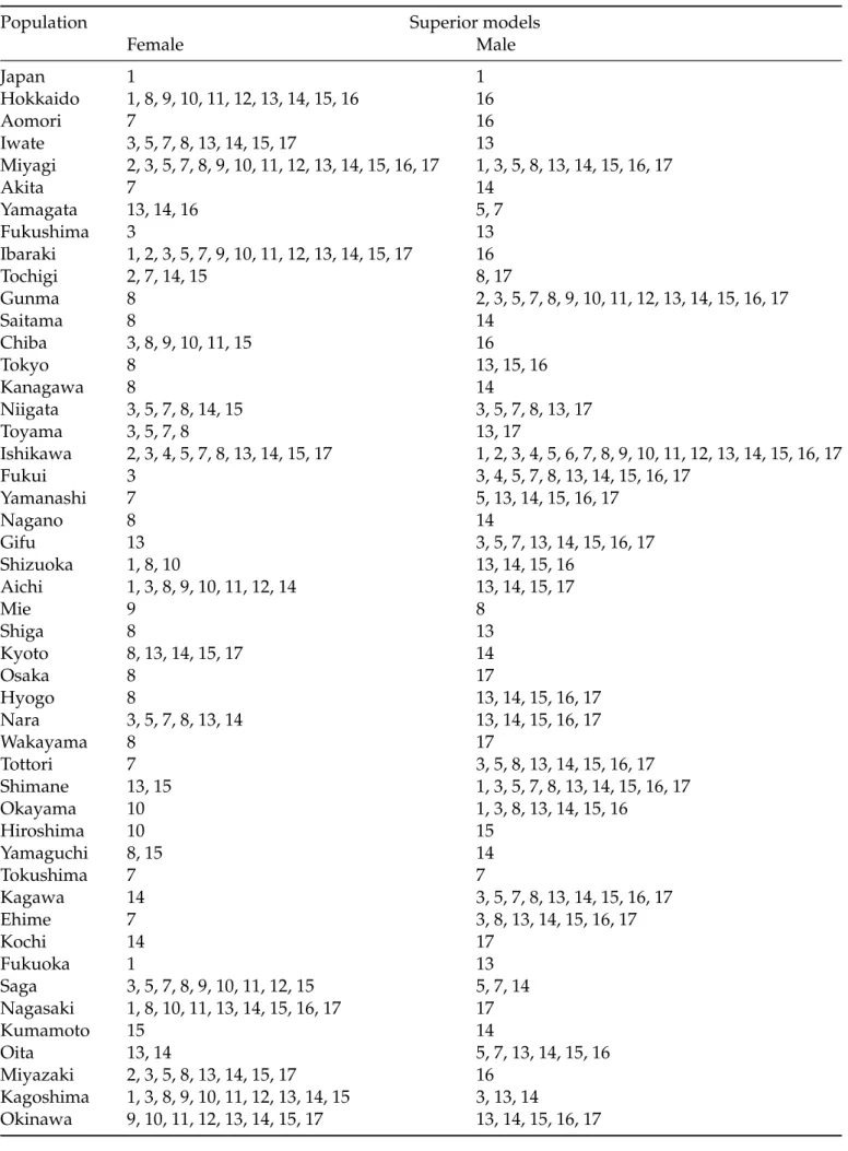
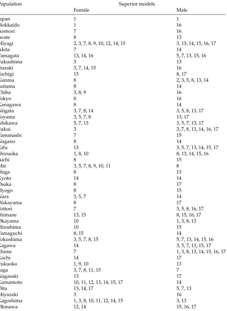
With the 90% confidence level of the MCS tests, we identify the set of superior models regarding point forecast accuracy. In Tables2and3, we determine the set of superior models among the 17 models considered using theTmax,MandTR,Mtests.

[Table 2 about here.]

[Table 3 about here.]

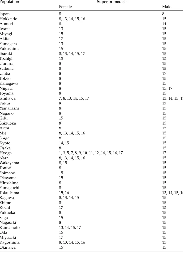
Based on the mean interval scores in the validation period, we examine statistical significance in interval forecast accuracy among the time-series extrapolation methods. With the 90% confidence level of the MCS tests, we identify the set of superior models regarding interval forecast accuracy. In Tables4and5, we determine the set of superior models using both theTmax,MandTR,Mtests

among the 17 models considered.

[Table 4 about here.]

5.4

Point and interval forecast comparison

Based on the selected set of superior models, we produce model-averaged point and interval forecasts using equal weights. In Table6, we compute the point and interval forecast accuracies for female and male data.

[Table 6 about here.]

As measured by the mean RMSFE over ten years in the forecasting period, the Plat model gives the most accurate point forecasts for the whole of Japan. For the average of 47 prefectures in Japan, the Plat model gives the most accurate point forecasts for females, while the multilevel functional time-series method performs the best for males. Although the model-averaging methods are not the best model, in this case, they rank among the top-performing methods. Between the two statistical significance tests, there is a marginal difference in the point forecast accuracy.

As measured by the mean interval scores over ten different horizons, the Plat model produces the most accurate interval forecasts for the whole of Japan and its prefectures for females. For males, the model-averaging methods perform the best for the whole of Japan and rank as the second best after the product-ratio method for the average of 47 prefectures. Again, there is a marginal difference between the two statistical significance tests regarding interval forecast accuracy.

6

A competing model averaging method

An existing model averaging method combines forecasts from the top two methods (seeShang,

2012). Given the top two methods are arbitrary from sample to sample, we have decided to combine forecasts from all methods and assign weights differently. Among all methods, we determine point or interval forecast accuracy as measured by the corresponding forecast errors in the validation set, and assign the weights to be the inverse of their forecast errors. We then standardize all weights so that the weights sum to 1. Conceptually, the method that performs better in the validation set receives a higher weight in the combined forecasts. The point and interval forecast accuracies of this model-averaging method are presented in Table7.

[Table 7 about here.]

Compared to our proposal model averaging method, the existing model averaging method assigns different weights to different models. From the in-sample forecast errors, the existing model averaging method assigns higher weights for those more accurate models and lower

weights for those less accurate models. By contrast, our proposed model averaging method selects a superior subset of models and assign equal weights. From the results, we find that the proposed model averaging method gives a smaller forecast error than the existing model averaging method.

7

Discussion

We first revisit four families of stochastic mortality models, namely the Renshaw-Haberman models, the Cairns-Blake-Dowd models, the Lee-Carter models, and the functional time-series models. From the viewpoint of actuarial science, mortality forecasts are an important input for determining annuity prices and reserves. From the viewpoint of demography, mortality forecasts are vital for policy-making at the national and national levels. Using the national and sub-national Japanese mortality rates, we evaluate and compare point and interval forecast accuracies, as measured by the root mean squared error and mean interval score, among the 17 time-series extrapolation methods and two model-averaging methods considered.

From the viewpoint of the point forecast accuracy, the Plat model gives the smallest point forecast errors, followed by the Lee-Carter and model-averaged method for Japanese females and males. In this case, because the superior set of the models was determined from in-sample forecast errors, it is the case where the best model for the in-sample forecasts may not be the best model for out-of-sample forecasts. This affects the forecast accuracy of the model-averaged method. Also, the Lee-Carter method with the Poisson error structure is more accurate than the version with the Gaussian error structure. For modeling sub-national Japanese females, the Plat model also performs the best; while the multilevel functional time-series model performs the best for males. From the viewpoint of the interval forecast accuracy, the Plat model gives the smallest interval forecast errors, followed by the model-averaged methods for Japanese females. For Japanese males, the model-averaged methods produce the smallest interval forecast errors for Japan and are on a par with the product-ratio method for Japanese sub-national data. To our surprise, the Renshaw-Haberman methods produce relatively worse interval forecast accuracy than that produced by the Lee-Carter and functional time-series methods. The result could be due to the instability of parameter estimation.

From Tables2,3and4,5, the best model for producing point forecasts does not necessary the same as the best model for producing interval forecasts, and the best model for producing the national series does not necessarily perform the best for the sub-national series, as the features of the data may be different.

method to select a set of superior model based on the model confidence set. The model confidence set is a procedure that determines a set of superior models based on the in-sample forecast errors.

For producing point forecasts, the selected superior sets of models are more diverse. For producing interval forecasts, the selected superior set of models often includes the product-ratio method, especially for male series. Given the product-ratio method is a joint modeling and coherent forecasting method, it achieves better forecast accuracy for males with a small sacrifice in terms of the female results. By coherent, we believe within each prefecture, female and male subpopulations share the similar characteristics, such as health facilities. Generally, the joint modeling methods, which also include the multivariate and multilevel functional time-series methods, often but not always outperform the model without incorporating correlation among subpopulations. The model-averaged forecasts may not perform the best for females and males, but they tend to give an aggregate best performance.

We show that potential gains in forecast accuracy can be achieved by discarding the worse per-forming models before combining the forecasts equally. By contrast, an existing model-averaging method assigning different weights for all models performs worse than the proposed method. We find that the proposed model-averaging method offers a more robust procedure for selecting the forecasting models based on their in-sample performances. By robustness, the model-averaged methods are protected against model misspecification. The advantage of the model-averaged methods is more apparent for males than females.

The accurate forecasting of mortality at retirement ages is essential to determine life, fixed-term and delayed annuity prices for various maturities and starting ages (see, e.g.,Shang and Haberman,2017). In the online supplement, we present a study on calculating single-premium fixed-term immediate annuity. To forecast mortality rates, we suggest considering the notion of model averaging.

In our modeling and analysis, we have made several choices. Below, we set out the ways in which the different choices could potentially have affected our results/overall conclusions.

1) We considered ages from 60 and 100+ to study the mortality pattern of retirees. We could apply the model averaging idea to other age groups,such as ages from 0 to 100+. With different age groups, the point and interval forecast results may be different.

2) Other age-specific mortality forecasting models could be incorporated into the model av-eraging. We consider only time-series extrapolation methods, and did not consider the expectation or explanation methods. For long-term forecasts and the expectation, expectation method has been used by theThe Institute and Faculty of Actuaries and the CMI(2018).

The inclusion of the expectation or explanation methods may alter the selection of superior models.

3) We modeled age-specific mortality rates, but the focus could also be on death counts or survival probabilities. For example, when we model age-specific death counts, there are other models, such as compositional data analysis, that could be included in the initial model pool.

4) After selecting the superior set of models, one could assign different weights instead of equal weights considered.With different weights, our forecast results may be improved as considered inShang(2012).

5) In applying the model confidence set procedure ofHansen et al. (2011), we consider the 90% confidence level. Considering other levels of confidence is possible. In general, as the confidence level increases, the number of superior models decreases.

6) We evaluated and compared one-step-ahead, five-step-ahead, and ten-step-ahead point and interval forecast accuracies. Considering other forecast horizons is also possible. For the longer term, the extrapolation methods may not perform well.

7) We evaluated point forecast accuracy by the root mean square error and interval forecast accuracy by the mean interval score and coverage probability deviance, respectively. Consid-ering other forecast error criteria, such as mean absolute percentage error or mean absolute scaled error, is also possible. With different error measures, the point and interval forecast results may be different.

We believe the present work paves the way for the above possible future research directions, and the proposed model-averaging method should be a welcome addition to the demographic modeling and forecasting.

SUPPLEMENTARY MATERIAL

Code for Shiny application The R code to produce a Shiny user interface for plotting every series in the Japanese human mortality data. (shiny.R)

Geography locations of the 47 prefectures in Japan We present a graphical display of the 47 pre-fectures within eight regions in Japan and include a table documenting the names of the 47 prefectures. (supplement MCS.pdf)

Detailed point and interval forecast results While Table6presents a summary of the point and interval forecast accuracies, we present the detailed forecast results for ten years in the forecasting period. (supplement MCS.pdf)

Calculation for single-premium fixed-term immediate annuity The forecasted mortality rate is an essential input for determining temporary annuity prices for various maturities and starting ages of the annuitant. (supplement MCS.pdf)

References

Abel, G. J., Bijak, J., Forster, J. J., Raymer, J., Smith, P. W. F. and Wong, J. S. T. (2013), ‘Integrating uncertainty in time series population forecasts: An illustration using a simple projection model’,

Demographic Research29, 1187–1226.

Aiolfi, M., Capistr´an, C. and Timmermann, A. G. (2010), Forecast combinations, Working paper 2010-21, CREATES.

URL:https://papers.ssrn.com/sol3/papers.cfm?abstract_id=1609530

Bates, J. M. and Granger, C. W. J. (1969), ‘The combination of forecasts’, Operational Research Quarterly20(4), 451–468.

Bernardi, M. and Catania, L. (2014), The model confidence set package for R, Technical report, Sapienza University of Rome.

URL:https://arxiv.org/abs/1410.8504

Bijak, J. (2011),Forecasting International Migration in Europe: A Bayesian View, Springer, New York.

Booth, H. (2006), ‘Demographic forecasting: 1980 to 2005 in review’,International Journal of Forecast-ing22(3), 547–581.

Booth, H., Hyndman, R. J., Tickle, L. and De Jong, P. (2006), ‘Lee-Carter mortality forecasting: A multi-country comparison of variants and extensions’,Demographic Research15, 289–310.

Booth, H., Maindonald, J. and Smith, L. (2002), ‘Applying Lee-Carter under conditions of variable mortality decline’,Population Studies56(3), 325–336.

Booth, H. and Tickle, L. (2008), ‘Mortality modelling and forecasting: A review of methods’,Annals of Actuarial Science3(1-2), 3–43.

Cairns, A. J. G., Blake, D. and Dowd, K. (2006), ‘A two-factor model for stochastic mortality with parameter uncertainty: Theory and calibration’,The Journal of Risk and Insurance73(4), 687–718.

Cairns, A. J. G., Blake, D., Dowd, K., Coughlan, G. D., Epstein, D. and Khalaf-Allah, M. (2011), ‘Mor-tality density forecasts: An analysis of six stochastic mor‘Mor-tality models’,Insurance: Mathematics & Economics48(3), 355–367.

Cairns, A. J. G., Blake, D., Dowd, K., Coughlan, G. D., Epstein, D., Ong, A. and Balevich, I. (2009), ‘A quantitative comparison of stochastic mortality models using data from England and Wales

Chiou, J.-M., Chen, Y.-T. and Yang, Y.-F. (2014), ‘Multivariate functional principal component analysis: A normalization approach’,Statistica Sinica24(4), 1571–1596.

Clayton, D. and Schifflers, E. (1987a), ‘Models for temporal variation in cancer rates. I: Age-period and age-cohort models’,Statistics in Medicine6(4), 449–467.

Clayton, D. and Schifflers, E. (1987b), ‘Models for temporal variation in cancer rates. II: Age-period-cohort models’,Statistics in Medicine6(4), 469–481.

Clemen, R. T. (1989), ‘Combining forecasts: A review and annotated bibliography’,International Journal of Forecasting5(4), 559–583.

Crawford, T., de Haan, R. and Runchey, C. (2008), Longevity risk quantification and management: A review of relevant literature, Technical report, Society of Actuaries.

URL:https://www.soa.org/research-reports/2009/research-long-risk-quant/

Cuesta-Albertos, J. A. and Febrero-Bande, M. (2010), ‘A simple multiway ANOVA for functional data’,Test19(3), 537–557.

Currie, I. D., Durban, M. and Eilers, P. H. C. (2004), ‘Smoothing and forecasting mortality rates’,

Statistical Modelling4(4), 279–298.

Denuit, M., Devolder, P. and Goderniaux, A. C. (2007), ‘Securitization of longevity risk: Pricing survivor bonds with Wang transform in the Lee-Carter framework’, The Journal of Risk and Insurance74(1), 87–113.

Dickinson, J. P. (1975), ‘Some statistical results in the combination of forecasts’,Operational Research Quarterly24(2), 253–260.

Fischer, I. and Harvey, N. (1999), ‘Combining forecasts: What information do judges need to outperform the simple average?’,International Journal of Forecasting15(3), 227–246.

Genre, V., Kenny, G., Meyler, A. and Timmermann, A. (2013), ‘Combining expert forecasts: Can anything beat the simple average?’,International Journal of Forecasting29(1), 108–121.

Girosi, F. and King, G. (2008),Demographic forecasting, Princeton University Press, Princeton.

Gneiting, T. and Katzfuss, M. (2014), ‘Probabilistic forecasting’,Annual Review of Statistics and Its Application1, 125–151.

Gneiting, T. and Raftery, A. E. (2007), ‘Strictly proper scoring rules, prediction and estimation’,

Graefe, A. (2015), ‘Improving forecasts using equally weighted predictors’,Journal of Business Research68(8), 1792–1799.

Haberman, S. and Renshaw, A. (2008), ‘Mortality, longevity and experiments with the Lee-Carter model’,Lifetime Data Analysis14(3), 286–315.

Haberman, S. and Renshaw, A. (2009), ‘On age-period-cohort parametric mortality rate projections’,

Insurance: Mathematics & Economics45(2), 255–270.

Haberman, S. and Renshaw, A. (2011), ‘A comparative study of parametric mortality projection models’,Insurance: Mathematics & Economics48(1), 35–55.

Hanewald, K., Post, T. and Gr ¨undl, H. (2011), ‘Stochastic mortality, macroeconomic risks and life insurer solvency’,The Geneva Papers on Risk and Insurance-Issues and Practice36(3), 458–475.

Hansen, P. R., Lunde, A. and Nason, J. M. (2011), ‘The model confidence set’,Econometrica79(2), 453– 497.

Hatzopoulos, P. and Haberman, S. (2009), ‘A parameterized approach to modeling and forecasting mortality’,Insurance: Mathematics and Economics44(1), 103–123.

Hatzopoulos, P. and Haberman, S. (2013), ‘Common mortality modeling and coherent forecasts. An empirical analysis of worldwide mortality data’,Insurance: Mathematics & Economics52(2), 320– 337.

Hunt, A. and Blake, D. (2014), ‘A general procedure for constructing mortality models’,North American Actuarial Journal18(1), 116–138.

Hyndman, R. and Booth, H. (2008), ‘Stochastic population forecasts using functional data models for mortality, fertility and migration’,International Journal of Forecasting24(3), 323–342.

Hyndman, R. J. (2017),demography: Forecasting Mortality, Fertility, Migration and Population Data. R package version 1.20.

URL:https://CRAN.R-project.org/package=demography

Hyndman, R. J., Booth, H. and Yasmeen, F. (2013), ‘Coherent mortality forecasting: the product-ratio method with functional time series models’,Demography50(1), 261–283.

Hyndman, R. J. and Shang, H. L. (2009), ‘Forecasting functional time series (with discussions)’,

Hyndman, R. and Ullah, M. (2007), ‘Robust forecasting of mortality and fertility rates: A functional data approach’,Computational Statistics & Data Analysis51(10), 4942–4956.

Jacques, J. and Preda, C. (2014), ‘Model-based clustering for multivariate functional data’, Compu-tational Statistics & Data Analysis71, 92–106.

Japanese Mortality Database (2017),National Institute of Population and Social Security Research. Avail-able athttp://www.ipss.go.jp/p-toukei/JMD/index-en.html(data downloaded on Septem-ber 1, 2017).

Koissia, M. C. (2006), ‘Longevity and adjustment in pension annuities, with application to Finland’,

Scandinavian Actuarial Journal2006(4), 226–242.

Lee, R. D. and Carter, L. R. (1992), ‘Modeling and forecasting U.S. mortality’,Journal of the American Statistical Association87(419), 659–671.

Lee, R. D. and Miller, T. (2001), ‘Evaluating the performance of the Lee-Carter method for forecast-ing mortality’,Demography38(4), 537–549.

Makridakis, S., Andersen, A., Carbone, R., Fildes, R., Hibon, M., Lewandowski, R., Newton, J., Parzen, E. and Winkler, R. (1982), ‘The accuracy of extrapolation (time series) methods: Results of a forecasting competition’,Journal of Forecasting1(2), 111–153.

Makridakis, S., Hibon, M. and Moser, C. (1979), ‘Accuracy of forecasting: An empirical investiga-tion’,Journal of the Royal Statistical Society: Series A142(2), 97–145.

Morris, J. S. and Carroll, R. J. (2006), ‘Wavelet-based functional mixed models’,Journal of the Royal Statistical Society: Series B68(2), 179–199.

Morris, J. S., Vannucci, M., Brown, P. J. and Carroll, R. J. (2003), ‘Wavelet-based nonparametric modeling of hierarchical functions in colon carcinogenesis’, Journal of the American Statistical Association98(463), 573–583.

Pitacco, E., Denuit, M., Haberman, S. and Olivieri, A. (2009),Modelling Longevity Dynamics for Pensions and Annuity Business, Oxford University Press, Oxford.

Plat, R. (2009a), ‘On stochastic mortality modeling’,Insurance: Mathematics & Economics45(3), 393– 404.

Plat, R. (2009b), ‘Stochastic portfolio specific mortality and the quantification of mortality basis risk’,Insurance: Mathematics and Economics45(1), 123–132.

Renshaw, A. E. and Haberman, S. (2003a), ‘Lee-Carter mortality forecasting with age-specific enhancement’,Insurance: Mathematics & Economics33(2), 255–272.

Renshaw, A. E. and Haberman, S. (2006), ‘A cohort-based extension to the Lee-Carter model for mortality reduction factors’,Insurance: Mathematics and Economics38(3), 556–570.

Renshaw, A. E. and Haberman, S. (2008), ‘On simulation-based approaches to risk measurement in mortality with specific reference to Poisson Lee-Carter modelling’,Insurance: Mathematics & Economics42(2), 797–816.

Renshaw, A. and Haberman, S. (2003b), ‘Lee-Carter mortality forecasting: A parallel generalized linear modelling approach for England and Wales mortality projections’, Journal of the Royal Statistical Society: Series C (Applied Statistics)52(1), 119–137.

Samuels, J. D. and Sekkel, R. M. (2017), ‘Model confidence sets and forecast combination’, Interna-tional Journal of Forecasting33(1), 48–60.

Shang, H. L. (2012), ‘Point and interval forecasts of age-specific life expectancies: A model averag-ing approach’,Demographic Research27, 593–644.

Shang, H. L. (2015), ‘Statistically tested ccomparison of the accuracy of forecasting methods for age-specific and sex-specific mortality and life expectancy’,Population Studies69(3), 317–335.

Shang, H. L. (2016), ‘Mortality and life expectancy forecasting for a group of populations in developed countries: A multilevel functional data method’, The Annals of Applied Statistics

10(3), 1639–1672.

Shang, H. L., Booth, H. and Hyndman, R. J. (2011), ‘Point and interval forecasts of mortality rates and life expectancy: A comparison of ten principal component methods’,Demographic Research

25, 173–214.

Shang, H. L. and Haberman, S. (2017), ‘Grouped multivariate and functional time series forecasting: An application to annuity pricing’,Insurance: Mathematics & Economics75, 166–179.

Shang, H. L. and Hyndman, R. J. (2017), ‘Grouped functional time series forecasting: An application to age-specific mortality rates’,Journal of Computational and Graphical Statistics26(2), 330–343.

Shang, H. L., Wi´sniowski, A., Bijak, J., Smith, P. W. F. and Raymer, J. (2014), Bayesian functional models for population forecasting,inM. Marsili and G. Capacci, eds, ‘Proceedings of the Sixth Eurostat/UNECE Work Session on Demographic Projections’, Istituto Nazionale di Statistica.

Shang, H. L. and Yang, Y. (2017), Grouped multivariate functional time series method: An applica-tion to mortality forecasting,inG. Aneiros, E. G. Bongiorno, R. Cao and P. Vieu, eds, ‘Functional Statistics and Related Fields’, Springer, pp. 233–241.

The Institute and Faculty of Actuaries and the CMI (2018), Continuous Mortality Investigation. Accessed at September 15, 2018.

URL:https://www.actuaries.org.uk/learn-and-develop/continuous-mortality-investigation

Tickle, L. and Booth, H. (2014), ‘The longevity prospects of Australian seniors: An evaluation of forecast method and outcome’,Asia-Pacific Journal of Risk and Insurance8(2), 259–292.

Villegas, A. M., Kaishev, V. K. and Millossovich, P. (2018), ‘StMoMo: An R package for stochastic mortality modeling’,Journal of Statistical Software84(3), 1–38.

Wi´sniowski, A., Smith, P. W. F., Bijak, J., Raymer, J. and Forster, J. (2015), ‘Bayesian population forecasting: Extending the Lee-Carter method’,Demography52(3), 1035–1059.

Zhang, J.-T. (2014),Analysis of Variance for Functional Data, Chapman & Hall, Boca Raton.

Zhao, B. B. (2012), ‘A modified Lee-Carter model for analysing short-base-period data’,Population Studies66(1), 39–52.

Zhao, B. B., Liang, X., Zhao, W. and Hou, D. (2013), ‘Modeling of group-specific mortality in China using a modified Lee-Carter model’,Scandinavian Actuarial Journal2013(5), 383–402.

Table 1: A list of the 19 models considered.

Family of models Label Model

Renshaw-Haberman 1 Lee-Carter model with Poisson error structure 2 Renshaw-Haberman model

3 Age-period-cohort model

Cairns-Blake-Dowe 4 Cairns-Blake-Dowe model 5 M6 model

6 M7 model 7 M8 model 8 Plat model

Lee-Carter 9 Lee-Carter model with Gaussian error structure 10 Booth-Maindonald-Smith model

11 Lee-Carter model with adjustment of life expectancy 12 Lee-Carter model with no adjustment to the score

Functional time series 13 Functional data model

14 Robust functional data model 15 Product-ratio model

16 Multivariate functional data model 17 Multilevel functional data model

Model averaging 18 MCS (Tmax,M) to select equal-weighted models

Table 2: MCS procedure using the Tmax,Mtest applied to the RMSFE in the validation set from 1996 to

2005 for forecasting the Japanese female and male national and sub-national mortality for ages between 60 and 100+. From the 17 models, below is the selected superior set of the model(s).

Population Superior models

Female Male Japan 1 1 Hokkaido 1, 8, 9, 10, 11, 12, 13, 14, 15, 16 16 Aomori 7 16 Iwate 3, 5, 7, 8, 13, 14, 15, 17 13 Miyagi 2, 3, 5, 7, 8, 9, 10, 11, 12, 13, 14, 15, 16, 17 1, 3, 5, 8, 13, 14, 15, 16, 17 Akita 7 14 Yamagata 13, 14, 16 5, 7 Fukushima 3 13 Ibaraki 1, 2, 3, 5, 7, 9, 10, 11, 12, 13, 14, 15, 17 16 Tochigi 2, 7, 14, 15 8, 17 Gunma 8 2, 3, 5, 7, 8, 9, 10, 11, 12, 13, 14, 15, 16, 17 Saitama 8 14 Chiba 3, 8, 9, 10, 11, 15 16 Tokyo 8 13, 15, 16 Kanagawa 8 14 Niigata 3, 5, 7, 8, 14, 15 3, 5, 7, 8, 13, 17 Toyama 3, 5, 7, 8 13, 17 Ishikawa 2, 3, 4, 5, 7, 8, 13, 14, 15, 17 1, 2, 3, 4, 5, 6, 7, 8, 9, 10, 11, 12, 13, 14, 15, 16, 17 Fukui 3 3, 4, 5, 7, 8, 13, 14, 15, 16, 17 Yamanashi 7 5, 13, 14, 15, 16, 17 Nagano 8 14 Gifu 13 3, 5, 7, 13, 14, 15, 16, 17 Shizuoka 1, 8, 10 13, 14, 15, 16 Aichi 1, 3, 8, 9, 10, 11, 12, 14 13, 14, 15, 17 Mie 9 8 Shiga 8 13 Kyoto 8, 13, 14, 15, 17 14 Osaka 8 17 Hyogo 8 13, 14, 15, 16, 17 Nara 3, 5, 7, 8, 13, 14 13, 14, 15, 16, 17 Wakayama 8 17 Tottori 7 3, 5, 8, 13, 14, 15, 16, 17 Shimane 13, 15 1, 3, 5, 7, 8, 13, 14, 15, 16, 17 Okayama 10 1, 3, 8, 13, 14, 15, 16 Hiroshima 10 15 Yamaguchi 8, 15 14 Tokushima 7 7 Kagawa 14 3, 5, 7, 8, 13, 14, 15, 16, 17 Ehime 7 3, 8, 13, 14, 15, 16, 17 Kochi 14 17 Fukuoka 1 13 Saga 3, 5, 7, 8, 9, 10, 11, 12, 15 5, 7, 14 Nagasaki 1, 8, 10, 11, 13, 14, 15, 16, 17 17 Kumamoto 15 14 Oita 13, 14 5, 7, 13, 14, 15, 16 Miyazaki 2, 3, 5, 8, 13, 14, 15, 17 16 Kagoshima 1, 3, 8, 9, 10, 11, 12, 13, 14, 15 3, 13, 14 Okinawa 9, 10, 11, 12, 13, 14, 15, 17 13, 14, 15, 16, 17

Table 3: MCS procedure using the TR,Mtest applied to the RMSFE in the validation set from 1996 to 2005

for forecasting the Japanese female and male national and sub-national mortality for ages between 60 and 100+.

Population Superior models

Female Male Japan 1 1 Hokkaido 1 16 Aomori 7 16 Iwate 8 13 Miyagi 2, 3, 7, 8, 9, 10, 12, 14, 15 3, 13, 14, 15, 16, 17 Akita 7 14 Yamagata 13, 14, 16 5, 7, 13, 15, 16 Fukushima 3 13 Ibaraki 3, 7, 14, 15 16 Tochigi 15 8, 17 Gunma 8 2, 3, 5, 8, 13, 14 Saitama 8 14 Chiba 3, 8, 9 16 Tokyo 8 16 Kanagawa 8 14 Niigata 3, 7, 8, 14 3, 5, 8, 13, 17 Toyama 3, 5, 7, 8 13, 17 Ishikawa 5, 7, 13 3, 5, 7, 13, 17 Fukui 3 3, 7, 8, 13, 14, 16, 17 Yamanashi 7 15 Nagano 8 14 Gifu 13 3, 5, 7, 13, 14, 15, 17 Shizuoka 1, 8, 10 8, 13, 14, 15, 16 Aichi 8 15 Mie 3, 5, 7, 8, 9, 10, 11 8 Shiga 8 13 Kyoto 14 14 Osaka 8 17 Hyogo 8 15 Nara 3, 5, 7 14 Wakayama 8 17 Tottori 7 3, 5, 8, 16, 17 Shimane 13, 15 8, 15, 16, 17 Okayama 10 1, 3, 8, 13 Hiroshima 10 15 Yamaguchi 8, 15 14 Tokushima 3, 5, 7, 8, 15 5, 7, 13, 14, 15, 16 Kagawa 14 3, 5, 7, 13, 15, 17 Ehime 7 1, 3, 8, 13, 14, 15, 16, 17 Kochi 14 17 Fukuoka 1, 9, 10 13 Saga 3, 7, 8, 11, 15 7 Nagasaki 13 17 Kumamoto 10, 11, 12, 13, 14, 15, 17 14 Oita 13, 14, 17 5, 7, 13 Miyazaki 3 16 Kagoshima 1, 3, 8, 10, 11, 12, 14, 15 3, 13 Okinawa 12, 14 15, 16, 17

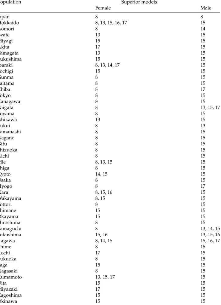
Table 4: MCS procedure using the Tmax,Mtest applied to the mean interval score in the validation set from

1996 to 2005 for forecasting the Japanese female and male national and sub-national mortality rates for ages between 60 and 100+.

Population Superior models

Female Male Japan 8 8 Hokkaido 8, 13, 14, 15, 16 15 Aomori 8 14 Iwate 13 15 Miyagi 15 15 Akita 17 15 Yamagata 13 15 Fukushima 15 15 Ibaraki 8, 13, 14, 15, 17 15 Tochigi 15 15 Gunma 8 15 Saitama 8 15 Chiba 8 17 Tokyo 8 15 Kanagawa 8 15 Niigata 8 15, 17 Toyama 8 15 Ishikawa 7, 8, 13, 14, 15, 17 13, 14, 15, 17 Fukui 8 13 Yamanashi 8 15 Nagano 8 15 Gifu 15 15 Shizuoka 8 15 Aichi 8 15 Mie 8, 13, 14, 15, 16 15 Shiga 8 15 Kyoto 14, 15 15 Osaka 8 15 Hyogo 1, 3, 5, 7, 8, 9, 10, 11, 12, 14, 15, 16, 17 17 Nara 8, 13, 14, 15, 16 15 Wakayama 8, 15 15 Tottori 8 15 Shimane 15 15 Okayama 15 15 Hiroshima 8 15 Yamaguchi 8 15 Tokushima 15, 16 13, 14, 15, 16 Kagawa 8, 13, 14, 15 15 Ehime 8 15 Kochi 17 15 Fukuoka 8 15 Saga 15 15 Nagasaki 8 15 Kumamoto 13, 14, 15, 17 15 Oita 15 15 Miyazaki 17 15 Kagoshima 8, 13, 14, 15, 16 15 Okinawa 15 15

Table 5: MCS procedure using the TR,Mtest applied to the mean interval score in the validation set from

1996 to 2005 for forecasting the Japanese female and male national and sub-national mortality rates for ages between 60 and 100+.

Population Superior models

Female Male Japan 8 8 Hokkaido 8, 13, 15, 16, 17 15 Aomori 8 14 Iwate 13 15 Miyagi 15 15 Akita 17 15 Yamagata 13 15 Fukushima 15 15 Ibaraki 8, 13, 14, 17 15 Tochigi 15 15 Gunma 8 15 Saitama 8 15 Chiba 8 17 Tokyo 8 15 Kanagawa 8 15 Niigata 8 13, 15, 17 Toyama 8 15 Ishikawa 13 15 Fukui 8 13 Yamanashi 8 15 Nagano 8 15 Gifu 8 15 Shizuoka 8 15 Aichi 8 15 Mie 8, 13, 15 15 Shiga 8 15 Kyoto 14, 15 15 Osaka 8 15 Hyogo 8 17 Nara 8, 15, 16 15 Wakayama 8, 15 15 Tottori 8 15 Shimane 15 15 Okayama 15 15 Hiroshima 8 15 Yamaguchi 8 13, 14, 15 Tokushima 15, 16 13, 15, 16 Kagawa 8, 14, 15 15, 16, 17 Ehime 8 15 Kochi 17 15 Fukuoka 8 15 Saga 15 15 Nagasaki 8 15 Kumamoto 13, 15, 17 15 Oita 15 15 Miyazaki 17 15 Kagoshima 15 15 Okinawa 15 15

Table 6: Point and interval forecast accuracies among the 17 models and two model-averaged methods in the Japanese national data and the average of 47 sub-national populations for ages between 60 and 100+. Forecast errors have been multiplied by 100. The smallest overall errors are shown in bold.

RMSFE Mean interval score

Series Method National data Sub-national data National data Sub-national data

Female 1 0.54 1.11 1.81 3.88 2 4.20 6.24 7.12 61.70 3 1.34 1.61 4.91 5.41 4 1.98 2.17 7.24 7.09 5 1.20 1.51 3.71 4.50 6 2.05 2.27 5.95 5.84 7 0.87 1.27 1.93 2.89 8 0.33 1.02 0.86 2.40 9 0.67 1.26 2.10 4.26 10 0.69 1.27 2.24 4.34 11 0.69 1.27 2.20 4.33 12 0.69 1.28 2.22 4.30 13 0.71 1.21 1.31 2.71 14 0.72 1.21 1.35 2.70 15 0.61 1.21 1.32 2.94 16 0.83 1.25 1.43 3.40 17 0.81 1.23 1.80 2.73 18 0.54 1.24 0.87 2.57 19 0.54 1.22 0.87 2.57 Male 1 0.71 2.55 2.79 9.56 2 2.27 4.02 7.97 14.57 3 1.93 3.13 8.17 11.40 4 2.92 3.76 12.18 13.01 5 1.78 2.96 6.42 9.45 6 2.75 3.69 9.72 10.47 7 1.60 2.84 3.81 7.91 8 0.65 2.47 1.37 5.77 9 0.99 3.78 3.68 12.80 10 1.00 3.76 3.80 12.78 11 1.02 3.83 3.91 13.05 12 1.00 3.47 3.63 10.88 13 0.72 2.51 1.50 5.86 14 0.78 2.51 1.49 5.87 15 0.72 2.47 1.98 5.02 16 0.93 2.47 1.79 7.23 17 0.76 2.44 1.79 5.49 18 0.71 2.51 1.36 5.06 19 0.71 2.50 1.36 5.07

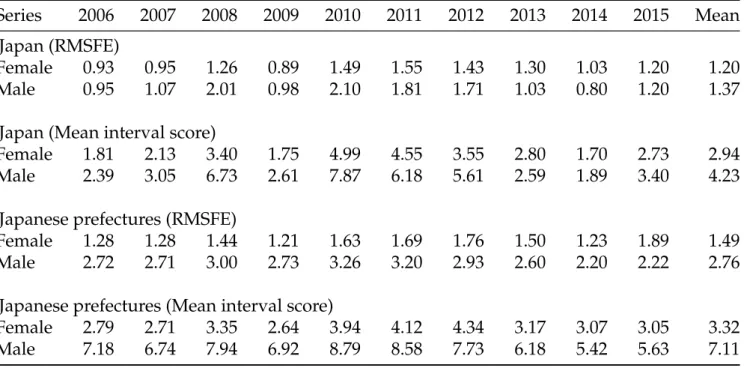
Table 7: Point and interval forecast accuracies for an existing model-averaged method averaged across the Japanese female and male national and sub-national mortality rates for ages between 60 and 100+. Forecast errors have been multiplied by 100. The results show its inferior point and interval forecast accuracies compared to the proposed two model-averaging methods. This further confirms that one should not average all models, but a subset of all ‘good’ models.

Series 2006 2007 2008 2009 2010 2011 2012 2013 2014 2015 Mean Japan (RMSFE)

Female 0.93 0.95 1.26 0.89 1.49 1.55 1.43 1.30 1.03 1.20 1.20 Male 0.95 1.07 2.01 0.98 2.10 1.81 1.71 1.03 0.80 1.20 1.37

Japan (Mean interval score)

Female 1.81 2.13 3.40 1.75 4.99 4.55 3.55 2.80 1.70 2.73 2.94 Male 2.39 3.05 6.73 2.61 7.87 6.18 5.61 2.59 1.89 3.40 4.23

Japanese prefectures (RMSFE)

Female 1.28 1.28 1.44 1.21 1.63 1.69 1.76 1.50 1.23 1.89 1.49 Male 2.72 2.71 3.00 2.73 3.26 3.20 2.93 2.60 2.20 2.22 2.76

Japanese prefectures (Mean interval score)

Female 2.79 2.71 3.35 2.64 3.94 4.12 4.34 3.17 3.07 3.05 3.32 Male 7.18 6.74 7.94 6.92 8.79 8.58 7.73 6.18 5.42 5.63 7.11