Significant wave height forecasting based on the hybrid EMD-SVM method
Kaixin Zhao & Jichao Wang∗
College of Science, China University of Petroleum, Qingdao 266580, China. ∗[E-mail: [email protected]]
Received 15 May 2018; revised 24 July 2018
Prediction of significant wave height (SWH) is considered an effective method in marine engineering and prevention of marine disasters. Support vector machine (SVM) model has limitations in processing nonlinear and non-stationary SWH time series. Fortunately, empirical mode decomposition (EMD) can effectively deal with the complicated series. So, the SWH prediction method based on EMD and SVM is proposed by combining the advantages of both methods. A statistical analysis was carried out to compare the results of two models i.e., between the hybrid EMD-SVM and SVM. In addition, two models are used for forecasting SWH with 3, 6, 12 and 24 hours lead times, respectively. A high R value of different prediction times for the hybrid model. Results indicate that SWH prediction of the hybrid EMD-SVM model is superior to the SVM model.
[Keywords: EMD-SVM model; Empirical mode decomposition; Significant wave height; Support vector machine]
Introduction
Prediction of significant wave height is essential for planning and operation of maritime activities and coastal engineering. Observation data of SWH can be
obtained from satellites, radars and buoys1 . And buoys
are considered the main reliable tool for acquiring
wave height data2. According to the different theories,
these methods of wave prediction are classified
into three types of approaches3-5 empirical-based,
numerical-based and soft-computing-based. Significant wave height series obtained from buoy located in the coastal region of China was used to train and test the proposed approaches.
Nowadays, in time series forecasting, different approaches based on soft computing have been widely used, and time taken for prediction is shorter than other conventional methods . Researchers have been using a nonlinear model based on soft computing technology, such as the artificial neural networks
(ANN) method was tested by Makarynskyy6 through
hourly observations of SWH in order to improve the accuracy of shortdated SWH forecast. Genetic algorithm for the prediction of SWH at three locations in the Bay of Bengal and the Arabian Sea, which compared with persistence forecasts and results indicate that the genetic algorithm prediction is
superior to persistence forecast7 . This model has been
used to predict the SWH by Cañellas et.al8 They
employed the genetic algorithm forecasting wave
height with other numerical models combined to
improve forecast accuracy. Kazeminezhad et.al9 has
predicted wave height using fuzzy inference system methods based on adaptive network and the accuracy of SWH predicted by the method has been improved.
Recently, a combination of different models has been observed for the increasing trend of SWH prediction. In this study, a hybrid approach, which combines the EMD and the SVM is proposed to
improve the quality of SWH forecasting. Duan et.al10
mentioned that if the SWH is a stationary time series, the recurrence map is evenly distributed. Otherwise, it is a non-uniform distribution. We know that the SWH is a nonlinear and non-stationary time series. So,
SVM, as a linear model11, has limitations in dealing
with SWH. EMD, as a novel soft-computing-based
method, was proposed by Huang et.al12 and has been
used widely through signal decomposition without any basis function. The key to this method is
empirical mode decomposition13, which decomposes
complex signals into finite intrinsic mode function (IMF). Local original signals at different time scales have been included in the decomposition of each IMF component. This method shows great effectiveness for the forecasting of SWH.
Materials and methods
The study area is located in the semi closed Bohai Sea. Bohai, is a shallow sea enclosed by Liaodong
and Shandong peninsula, lies in the northernmost tip of the eastern part of the mainland of China, which faces the sea on the side and surrounds the land on three sides.
In this area, every hour wave height data was collected from Dec., 15, 2012 to Feb., 15, 2013 by a
buoy at 121°40'48'' E and 38°9'31'' N (Fig. 1) totaling
1290 records. In order to predict SWH for short-term, we divided the buoy data set from Bohai into training and testing data. The data of 810 records are selected as the training set and the remaining 480 data are utilized as the test set. It is worth mentioning that the data sets were missing between Dec.28, 2012 and Jan. 2013.
Support vector machine
SVM as a new soft-computing method has gained a reputation . Based on the vc dimension theory, the
method was first proposed by Vapnik13,14. The SVM
model has many unique advantages in solving the problems of pattern recognition, classification and
regression analysis1. Regional training error was
minimized by the traditional method, whereas the SVM model focused on minimizing of the
generalization errors13,14.
In the regression problem, the appropriate function had to be found which can approximate predicted value in the given data. Due to the convexity of the
problem, the unique solution is given1. The basic idea
of SVM is tantamount to map the training data into a high dimensional space of kernel function, which can make the training data linearization.
Optimization problems with support vector machines:
Original space: 𝑇 = {(𝑥 , 𝑦 ), ⋯ , (𝑥 , 𝑦 )}
Get the Hilbert H space corresponding to the new
training set:
𝑇 = {(𝑥 , 𝑦 ), ⋯ , (𝑥 , 𝑦 )} = {(𝜙(𝑥 ), 𝑦 ), ⋯ , (𝜙(𝑥 ), 𝑦 )}
The hyperplane (𝜔 ⋅ 𝑥) + 𝑏 = 0 in the H space.
This space can be divided into corresponding training set, and the training set for the super plane geometric interval reaches maximum.
min ∈ , ∈ , ∈ 1 2∥ 𝜔 ∥ + 𝑐 𝜉 s.t. 𝑦 ((𝜔 ⋅ 𝑥 ) + 𝑏) ≥ 1 − 𝜉 𝑖 = 1, ⋯ , 𝑙 𝜉 ≥ 0 𝑖 = 1, ⋯ , 𝑙.
where (𝑥 , 𝑦 ), 𝑖 = 1, ⋯ , 𝑙 by the formula given, 𝑐 ≥ 0
and 𝑐 represents the error penalty factor.
The dual problem can ben obtained by using Lagrange multiplier algorithm. Now introduce the
Lagrange multiplier 𝑎: min1 2 𝑦 𝑦 𝑎 𝑎 𝐾(𝑥 ⋅ 𝑥 ) − 𝑎 s.t. 𝑦 𝑎 = 0 0 ≤ 𝑎 ≤ 𝑐 𝑖 = 1, ⋯ , 𝑙
where 𝐾(𝑥 , 𝑥 ) = 𝜙(𝑥 )𝜙(𝑦 ) and 𝐾(𝑥 , 𝑥 ) is the
kernel function, which is obtained from the two inner
vectors 𝑥 and 𝑥 in the feature spaces 𝜙(𝑥 ) and
𝜙(𝑦 ), respectively. The kernel function technique
can transform the nonlinear operation of low dimensional space into high dimensional space and simplify the operation.
Four basic kernel functions provided by the SVM model are polynomial, sigmoid, linear and radial.
Among them, the radial basis function (RBF)15 kernel
function is most beneficial and has less numerical difficulties. Therefore, this study adopts RBF, which can be represented as:
𝐾(𝑥 , 𝑥 ) = 𝑒𝑥𝑝(−𝛾 ∥ 𝑥 − 𝑥 ∥ )
where 𝑥 ∈ 𝑅 , variables 𝑥 and 𝑥 are input space
vectors and 𝛾 is the parameter of RBF kernel
function. The prediction accuracy of the RBF kernel
is determined by these parameters ( 𝛾 and 𝐶 ). For
optimizing the parameters 𝛾 and 𝐶 , the cross
validation strategy16, as a common technique, was
used to select the best matched parameters to evaluate learning algorithms. Cross validation was satisfied as far as possible: 1) the proportion of the training set should be enough, generally more than half; 2) the training set and testing set should be sampled evenly.
Hybrid EMD-SVM model
As is known to all, the EMD can effectively deal
with non-stationary and nonlinear signals13 such as
wave height data. EMD has been based on the SWH data of the characteristic time scale for signal decomposition without any basis function. SWH signal can be decomposed by the EMD into several stationary IMFs with different frequencies, according to its intrinsic characteristics.
Figure 2 shows the original signal characteristic of experimental data (contain 1290 records). This model is feasible for the analysis of signal sequences which is nonlinear and non-stationary. The purpose of the EMD model is to decompose the signal into the superposition of multiple IMFs, and the IMFs must
match with the following criterias12: (1) the number of
local extreme points and zero crossings in the whole time range must be equal or differ to one; (2) at any moment, the upper envelope and the mean envelope must be zero on average.
Suppose the wave height time sequence 𝑥(𝑡), the
algorithm shown as follows17:
(1) The upper and lower extremes of the 𝑥(𝑡) are
found, and the upper and lower envelopes are formed by using the three spline interpolation respectively.
Then, the initial value 𝑚 (𝑡) is calculated.
(2) The mean value of the upper and lower envelope
is calculated as 𝑚 (𝑡), and the original data sequence
𝑥(𝑡) minus the mean can be obtained by removing the
new data sequence ℎ (𝑡): 𝑥(𝑡) − 𝑚 (𝑡) =ℎ (𝑡).
(3) Generally, ℎ (𝑡) is not a IMF component sequence,
it is necessary to repeat this process 𝑘 times until the
mean value tends to zero, so that we get first IMF
components 𝑐 (𝑡).
(4)The 𝑐 (𝑡) is separated from the 𝑥(𝑡) to get a
different signal to remove the high frequency
component: 𝑟 (𝑡) = 𝑥(𝑡) − 𝑐 (𝑡).
(5) Using 𝑟 (𝑡) as the original data, repeat steps (1),
(2), and (3) to get second IMF components 𝑐 (𝑡).
Then repeat n times and get n IMF components
(𝑖𝑚𝑓 (𝑡) = 𝑐 (𝑡)): 𝑟 (𝑡) = 𝑥(𝑡) − 𝑐 (𝑡).
When 𝑐 (𝑡) or 𝑟 (𝑡) satisfies the termination
condition (usually 𝑟 (𝑡) becomes a monotone
function), the end of the cycle, can be obtained from the above formula:
𝑥(𝑡) = ∑ 𝑖𝑚𝑓 (𝑡) + 𝑟 (𝑡).
The 𝑟 (𝑡) is called the residual function (also
known as the trend term), which represents the average trend of the signal.
Hybrid EMD-SVM model establishment steps: (1) The EMD model method is used to decompose the SWH signal to obtain the IMFs component of the finite stationary signal.
(2) Normalize each component and the processed sequence can be divided into training set and testing set; (3) SVM prediction models are established respectively for the training set of each component, the testing sets are predicted with the new model. And the prediction set is reversely normalized.
(4) The final prediction results are achieved through the optimal weighted combination of the each component predicted values.
Evaluating accuracy of proposed models
It is the primary problem to determine which prediction model is superior to other model. The performance of the prediction model is usually evaluated by statistical standards: the root mean
square error18-20 (RMSE), coefficient of correlation19
(R) and agreement of index (IA) can compare the
performance of the models. Meanwhile, the RMSE
and R respectively represent the deviation and
interconnection between the observed and predicted SWH. These statistics are defined as:
𝑅𝑀𝑆𝐸 = 1
𝑛 (𝑥 − 𝑦 ) /
𝑅 = ∑ (𝑥 − 𝑥̅ ) ⋅ (𝑦 − 𝑦 ) ∑ (𝑥 − 𝑥̅ ) ⋅ (𝑦 − 𝑦 ) Fig. 2 — Original signal.
𝐼𝐴 = 1 − ∑ (𝑦 − 𝑥 ) ∑ (|𝑦 − 𝑥̅ | + |𝑥 − 𝑥̅ |)
where 𝑥 (𝑦) is the observed (predicted) result with
the mean value of 𝑥̅ (𝑦). n represents the total
number of data points used in the test.
Results
Historically SWH at buoy of the hybrid EMD-SVM and single SVM models with lead times of 3, 6, 12 and 24 hours are shown, respectively, in Figures 3, 4, 5 and 6 by the way of a representative sample.
And the forecasting results of the hybrid EMD-SVM model are compared with the EMD-SVM model by
the error statistics, including RMSE, R and IA. The
error statistics of the two models for testing data are given in Table 1. As can be seen, the prediction results of the hybrid EMD-SVM model are superior to
the single SVM model, regardless of RMSE, R or IA.
Fig. 3 — 3 hours prediction of SWH by the SVM and EMD-SVM.
Fig. 4 — 6 hours prediction of SWH by the SVM and EMD-SVM.
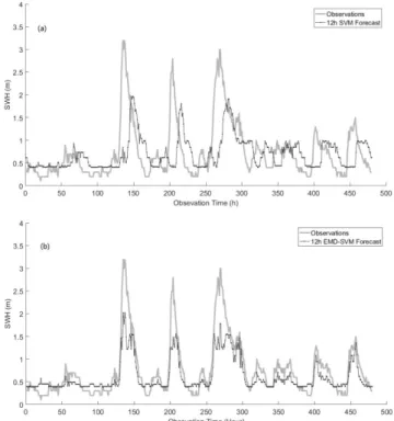
Fig. 5 ― 12 hours prediction of SWH by the SVM and EMD-SVM.
Fig. 6 — 24 hours prediction of SWH by the SVM and EMD-SVM.
Table 1 — Compare between the SVM model and the EMD-SVM model
SVM EMD-SVM
TIME RMSE R IA RMSE R IA
3H 0.2900 0.8872 0.9376 0.1583 0.9727 0.9813 6H 0.4628 0.6821 0.8076 0.2814 0.9228 0.9343 12H 0.6178 0.3021 0.5199 0.3718 0.9031 0.8517 24H 0.6773 -0.0485 0.2742 0.4499 0.9007 0.7920
Discussion
Using the hybrid SVM-EMD and single SVM models to prediction the significant wave height, respectively. This section provides the predicted SWH results from the EMD-SVM and SVM model. Fig. 3 shows the EMD-SVM model for predicting SWH is almost completely coincident with the actual observations within a lead time of 3 hours. In comparison, there is a certain difference between the prediction and the obsercation of the SVM model. It is worth noting that the predictions of the two models in a short lead of time (3 hours) can indicate the trend of the observed values, both of them are
underestimated in the peaks10. Meanwhile, the RMSE
parameters for the SWH by the SVM and hybrid EMD-SVM models were 0.2900 and 0.1583, while
the same for the R values were 0.8872 and 0.9727
(Table 1) in the prediction of lead times with 3 hours.
Further, the IA values of 0.9376 and 0.9813 were
obtained for the EMD-SVM and SVM model predictions, respectively (Table 1).
As presented in Fig. 3 and 4, for one thing, the observed values were well predicted by the EMD-SVM model in the forecasting time history of 400-480h. For another thing, with the increase of forecast time, the prediction results of the SVM model have obvious hysteresis. These shortcomings were clearly improved by using EMD-SVM model in forecasting
SWH. Taking errors statistics in Table 1, RMSE, R
and IA of 6-h predictions by the SVM model were
0.4628, 0.6821 and 0.8076, while those by the EMD-SVM model were 0.2814, 0.9228 and 0.9343, respectively. With the increase of forecasting horizon
times, the R and IA parameters decrease as the RMSE
values increase. However, the rate of deterioration of the hybrid EMD-SVM model is slower than the single SVM model.
Fig. 5 and 6 implied that the prediction effects of SVM model for 12 and 24 hours significant wave height were obviously unsatisfactory, which can also be apparent from Table 1. However, the EMD-SVM
model still forecasting the changes of peaks and troughs of SWH in the same prediction time.
Particularly, the R value of -0.0485 for 24 hours
prediction by the SVM model was terrible, while the same error statistic of the EMD-SVM model was 0.9007. When the output parameters of the SVM and EMD-SVM models were 24 forecasting hours SWH,
the RMSEwas 0.6773 and 0.4499, IA was 0.2742 and
0.7920, respectively. As can be seen by compared, the predicted results using the hybrid EMD-SVM are closer to the observed SWH than those using the SVM model for forecasting.
Conclusion
Results from this study indicate that the hybrid EMD-SVM model prediction can be proved superior to the SVM model. With the increase of forecast time, the prediction results of the SVM model have obvious hysteresis. These shortcomings were clearly improved by using EMD-SVM model in the prediction of SWH. In addition, peak predictions of the two models become more and more unsatisfactory with the increase of prediction time in advance. However, the rate of deterioration of the hybrid EMD-SVM model is slower than the single SVM model. It was found
that a higher R value of different prediction times for
the hybrid model, especially the 24 forecasting hours.
However, the same error statistic R of the SVM model
was a negative value, that is -0.0485.
Acknowledgement
Authors thank the National Key Research and Development Project of China (No.2016YFC1401800), the Fundamental Research Funds for the Central Universities (No.17CX02060 and 19CX05003A-5) and the National Natural Science Foundation of China (No.41406007).
References
1 Roy, C., Motamedi, S., Hashim, R., Shamshirband, S., Petkovic, D., A comparative study for estimation of wave height using traditional and hybrid soft-computing methods.
Environ. Earth.Sci., 75(2016):1-12.
2 Battjes, J.A., Computation of set-up, longshore currents, run-up and overtopping due to wind-generated waves. Ph.D. thesis, Technische hogeschool, Delft,1974.
3 Mahjoobi, J., Etemad-Shahidi, Kazeminezhad, M.H., Hindcasting of wave parameters using different soft computing methods. Appl.Ocean. Res., 30(2008):28-36. 4 Thirumalaiah, K., Deo M.C., Hydrological forecasting using
neural networks. J. Hydrol. Eng., 5(2000):180-189.
5 Jain , P., Garibaldi , J.M., Hirst, J.D., Supervised machine learning algorithms for protein structure classification.
6 Makarynskyy, O., Improving wave predictions with artificial neural networks. Ocean Eng., 31(2004):709-724.
7 Basu, S., Sarkar, A., Satheesan, K., Kishtawal, C.M., Predicting wave heights in the north Indian Ocean using genetic algorithm. Geophys. Res. Lett., 32(2005): L17608.
8 Cañellas, B., Balle, S., Tintoré J, Orfila, A., Wave height prediction in the Western Mediterranean using genetic algorithms. Ocean Eng., 37(2010):742-748.
9 Kazeminezhad, M.H., Etemad-Shahidi, A., Mousavi, S.J., Application of fuzzy inference system in the prediction of wave parameters. Ocean Eng., 32(2005):1709-1725. 10 Duan, W.Y., Han, Y., Huang, L.M., Zhao, B.B., Wang, M.H.,
A hybrid EMD-SVR model for the short-term prediction of significant wave height. Ocean Eng., 124(2016):54-73. 11 Ladicky, L., Torr, P.H.S., Locally Linear Support
Vector Machines. Appearing in Proceedings of the 28th International Conference on Machine Learning, USA, 2011. 12 Huang, N.E., Shen, Z., Long, S.R., Wu, M.W., Shih, H.H., Zheng, Q., Yen, N.C., Tung, C.C., Liu, H.H., The empirical mode decomposition and the Hilbert spectrum for nonlinear and non-stationary time series analysis.
Proc. R. Lond. Ser. A, 454(1998):903-995.
13 Vapnik, V., The Nature of Statistical Learning Theory.(Springer,New York), 1995,pp.314.
14 Vapnik, V., Statistical Learning Theory,vol.2.(Wiley, New York),1998, pp.391-394.
15 Mahjoobi, J., Ehsan Adeli Mosabbeb, Prediction of significant wave height using regressive support vector machines. Ocean Eng., 36 (2009):339-347.
16 Shao, J., Linear Model Selection by Cross-validation. J. Am. Stat. ssoc., 88 (1993):486-494.
17 Duan, W.Y., Huang, L.M., Han, Y., Huang, D., A hybrid EMD-AR model for nonlinear and non-stationary wave forecasting. J. Zhejiang. Univ. Sci. A, 17(2015):115-129. 18 Altunkaynak, A., AssefaNigussie T., Prediction of
daily rainfall by a hybrid wavelet-season-neuro technique.
J. Hydrol., 529(2015):287-301.
19 Berbić J, Ocvirk, E., Carević D, Lončar, G., Application of neural networks and support vector machine for significant wave height prediction. Oceanologia, 59(2017):331-349.
20 Deka, P.C., Prahlada R., Discrete wavelet neural network approach in significant wave height forecasting for multistep lead time. Ocean Eng., 43( 2012): 32-42.