Dynamic Operational Risk Assessment with Bayesian Network

i DYNAMIC OPERATIONAL RISK ASSESSMENT WITH BAYESIAN NETWORK

A Thesis by

SHUBHARTHI BARUA

Submitted to the Office of Graduate Studies of Texas A&M University

in partial fulfillment of the requirements for the degree of MASTER OF SCIENCE

August 2012

ii DYNAMIC OPERATIONAL RISK ASSESSMENT WITH BAYESIAN NETWORK

A Thesis by

SHUBHARTHI BARUA

Submitted to the Office of Graduate Studies of Texas A&M University

in partial fulfillment of the requirements for the degree of MASTER OF SCIENCE

Approved by:

Chair of Committee, M. Sam Mannan Committee Members, Carl D. Laird

Martin A. Wortman Head of Department, Charles J. Glover

August 2012

iii ABSTRACT

Dynamic Operational Risk Assessment with Bayesian Network. (August 2012) Shubharthi Barua, B.Sc., Bangladesh University of Engineering & Technology

Chair of Advisory Committee: Dr. M. Sam Mannan

Oil/gas and petrochemical plants are complicated and dynamic in nature. Dynamic characteristics include ageing of equipment/components, season changes, stochastic processes, operator response times, inspection and testing time intervals, sequential dependencies of equipment/components and timing of safety system operations, all of which are time dependent criteria that can influence dynamic processes. The conventional risk assessment methodologies can quantify dynamic changes in processes with limited capacity. Therefore, it is important to develop method that can address time-dependent effects. The primary objective of this study is to propose a risk assessment methodology for dynamic systems. In this study, a new technique for dynamic operational risk assessment is developed based on the Bayesian networks, a structure optimal suitable to organize cause-effect relations. The Bayesian network graphically describes the dependencies of variables and the dynamic Bayesian network capture change of variables over time. This study proposes to develop dynamic fault tree for a chemical process system/sub-system and then to map it in Bayesian network so that the developed method can capture dynamic operational changes in

iv process due to sequential dependency of one equipment/component on others. The

developed Bayesian network is then extended to the dynamic Bayesian network to demonstrate dynamic operational risk assessment. A case study on a holdup tank problem is provided to illustrate the application of the method. A dryout scenario in the tank is quantified. It has been observed that the developed method is able to provide updated probability different equipment/component failure with time incorporating the sequential dependencies of event occurrence. Another objective of this study is to show parallelism of Bayesian network with other available risk assessment methods such as event tree, HAZOP, FMEA. In this research, an event tree mapping procedure in Bayesian network is described. A case study on a chemical reactor system is provided to illustrate the mapping procedure and to identify factors that have significant influence on an event occurrence. Therefore, this study provides a method for dynamic operational risk assessment capable of providing updated probability of event occurrences considering sequential dependencies with time and a model for mapping event tree in Bayesian network.

v DEDICATION

My teachers,

Dr. M. Sam Mannan & Late Sushil Bhattachariya My parents,

Sathi Priya Barua & Sudipa Barua My sister,

Shatabdi Barua My friends,

vi ACKNOWLEDGEMENTS

I would like to express my gratitude to my committee chair, Dr. M. Sam Mannan, the person of my inspiration to work in the field of process safety. I would also like to thank him for giving me the opportunity to work in different industrial projects which helped me to build up teamwork skills, and to attend several meetings and continuing education courses which helped me to improve my communication skills. I would like to thank my committee members Dr. Carl D. Laird and Dr. Martin A. Wortman for the consent to be my committee members and continuous support. I would like to mention Dr. Hans J. Pasman for his time to discuss the scope of my research, provide background information on Bayesian networks, teaching me to use different software, reading my manuscripts, giving suggestions and comments. I would also like to thank my team leader Dr. Xiaodan Gao and Dr. Subramanya Nayak for their assistance, effort, time and valuable suggestions on my research. Also, I would like to express gratitude Dr. William J. Rogers and Dr. Xiaole Yang for their support in conducting this study.

I would like to express my gratitude to my parents, Engr. Sathi Priya Barua and Sudipa Barua, and my younger sister, Shatabdi Barua, for their constant love, unconditional care and consistent support from my childhood to become a better person and encouraging me to pursue MS degree in USA. I would like to mention Dr. Syed Faiyaz Hossainy, a family friend, for his generous support of my higher study in USA. I would also like to express sincere appreciation to my friends, Amira Yousuf Chowdhury

vii and Mir Abdul Karim, for providing me constant support from my undergrad study and

continuing it in MS course of study.

I would also like to acknowledge Valerie Green, Donna Startz and all staff of Mary Kay O’Connor Process Safety Center for their assistance on administrative issues. Also, I want to mention that I have learnt a lot from Dr. Victor Carreto Vazquez and Dr. Dedy NG while working with them in different projects. Assistance, guidance and suggestions from all my friends at Mary Kay O’Connor Process Safety Center have helped me to conduct this study, different projects and job-search. Finally, I must mention and thank all Bangladeshi students of Texas A&M University and their families living at College Station, Texas for being supportive in my personal life for last 2 years.

vii i TABLE OF CONTENTS Page ABSTRACT ... iii DEDICATION ... v ACKNOWLEDGEMENTS ... vi

TABLE OF CONTENTS ... viii

LIST OF FIGURES ... x 1. INTRODUCTION ... 1 1.1 Background ... 1 1.2 Problem Statement ... 3 1.3 Research Objective ... 4 1.4 Research Contributions ... 5

1.5 Organization of This Thesis ... 8

2. LITERATURE REVIEW ... 10

2.1 General Background ... 10

2.2 Conventional Risk Assessment Methodologies ... 11

2.3 Dynamic Risk Assessment Methods ... 15

2.4 Overview of Bayesian Network Applications ... 17

3. THE DEVELOPMENT OF BAYESIAN NETWORK BASED DYNAMIC OPERATIONAL RISK ASSESSMENT METHODOLOGY ... 19

3.1 Introduction ... 19

3.2 Research Framework ... 28

4. APPLICATION OF THE METHODOLOGY ... 47

4.1 Case Study: A Tank Holdup Problem ... 47

4.2 Application of the Model ... 68 LIST OF 7$%/(6 ... xLLL

ix Page

5.1 Introduction ... 75

5.2 Event Tree Mapping into Bayesian Network and Generalization Technique ... 75

5.3 Case Study ... 81

6. SUMMARY AND RECOMMENDATIONS ... 92

REFERENCES ... 95

VITA ... 103

x LIST OF FIGURES

Page Figure 1. Researches on dynamic operational risk assessment and Bayesian

statistics in MKOPSC ... 7

Figure 2. Functional/probabilistic dependency gate ... 21

Figure 3. Spare gates ... 22

Figure 4. Probability AND-Gate (PAND gate) ... 24

Figure 5. A simple Bayesian network ... 26

Figure 6. Framework for the dynamic Bayesian network based dynamic operational risk assessment method ... 30

Figure 7. Mapping algorithm of AND-gate and OR-gate in Bayesian network ... 33

Figure 8. Spare gates of dynamic fault tree mapping in dynamic Bayesian network (Montani et al., 2005) ... 36

Figure 9. Spare gates of dynamic fault tree with intermediate inputs mapping in dynamic Bayesian network ... 39

Figure 10. FDEP/PDEP gate mapping in dynamic Bayesian network (Montani et al., 2005) ... 41

Figure 11. A holdup tank (level control system) problem ... 50

Figure 12. Dynamic fault tree for the holdup tank problem ... 52

Figure 13. Root nodes, intermediate nodes and top event nodes in Bayesian network ... 54

xi Page

Figure 15. Dynamic Bayesian network with two time-slices without

connection among nodes of two time-slices ... 58 Figure 16. Mapped spare gate in dynamic Bayesian network ... 59 Figure 17. Dynamic Bayesian network with two time-slices ... 60 Figure 18. Dry-out probability upon different equipment/components failure

using different inspection intervals: weekly, monthly, 3 months, 6

months, 1 year and every 2 year ... 63 Figure 19. Less or no flow occurrence, automatic protection system failure

and outlet valve fails open (failure) probability using different inspection intervals: weekly, monthly, 3 months, 6 months, 1 year

and every 2 year ... 64 Figure 20. Pump system failure and pipe leakage probability using different

inspection intervals ... 65 Figure 21. Primary pump and its system components failure probability using

different inspection intervals ... 66 Figure 22. Standby Pump and its system components failure probability using

different inspection intervals ... 67 Figure 23. Dynamic Bayesian network when maintenance/repair is performed

at every 3 months interval (3 months, 6 months etc.) ... 69 Figure 24. Dryout probability in the system with no maintenance,

maintenance work in every 3 months and in every 6 months ... 72 Figure 25. Less or no flow probability in the system with no maintenance,

maintenance work in every 3 months and in every 6 months ... 72 Figure 26. Automatic protection system failure probability in the system with

no maintenance, maintenance in every 3 months and in every 6

months ... 73 Figure 27. Pump system failure probability in the system with no

maintenance, maintenance work in every 3 months and in every 6

xii Page

Figure 28. A general event tree ... 77

Figure 29. A general event tree mapped in Bayesian network ... 78

Figure 30. A chemical reactor system (Crowl and Louvar, 2002) ... 82

Figure 31. An event tree of a chemical reactor system ... 83

Figure 32. Mapped event tree in Bayesian network ... 84

xii

i

LIST OF TABLES

Page Table 1 Conditional probability table for primary component state at

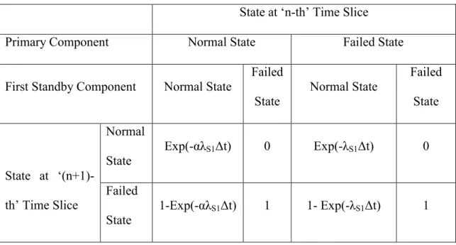
‘(n+1)-th’ time slice given its state at ‘n-th’ time slice ... 36 Table 2 Conditional probability table for the first standby component state

at ‘(n+1)-th’ time slice given the state of primary component and

first standby component at ‘n-th’ time slice ... 37 Table 3 Conditional probability for second standby component state at

‘(n+1)-th’ time slice given state of primary component, first

standby and second standby components state at ‘n-th’ time slice ... 38 Table 4 Conditional probability table for primary component state at

‘(n+1)-th’ time slice given its state at ‘n-th’ time slice for spare

gate as in figure 9 ... 40 Table 5 Conditional probability table for standby component state at

‘(n+1)-th’ time slice given its state at ‘n-th’ time slice for spare

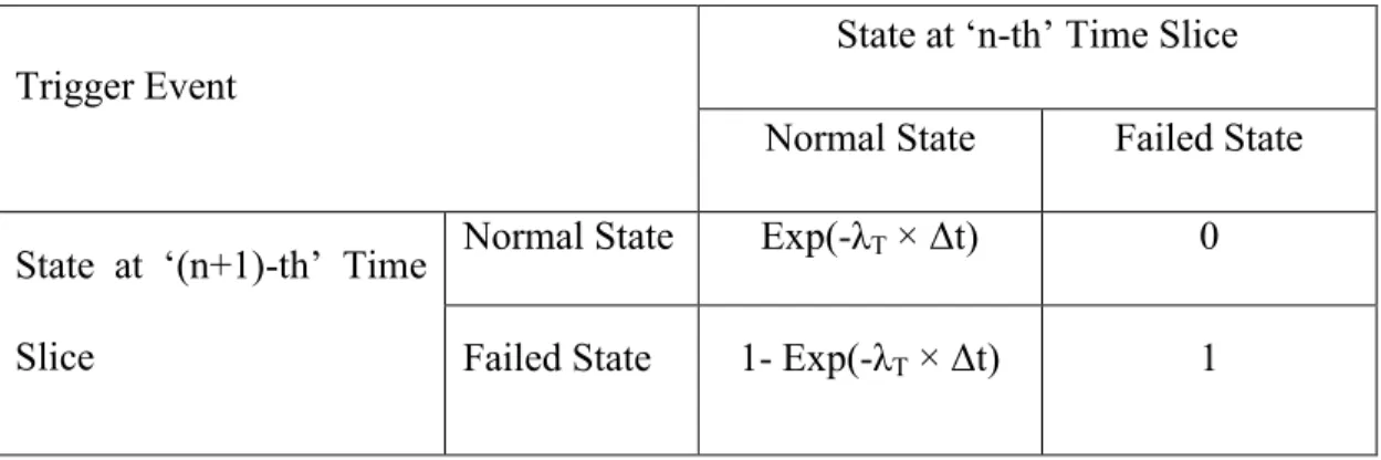
gate as in figure 9 ... 40 Table 6 Conditional probability table for trigger event at ‘(n+1)-th’ time

slice given its state at ‘n-th’ time slice ... 42 Table 7 Conditional probability table for dependent components at

‘(n+1)-th’ time slice given the state of trigger event at ‘n-‘(n+1)-th’ time slice ... 43 Table 8 Conditional probability table for component ‘X’ at ‘(n+1)-th’ time

slice given its state at ‘n-th’ time slice ... 44 Table 9 Component failure mode and failure rate data... 51 Table 10 Prior probabilities of root nodes of first time slice at 1 Week ... 61

xiv Page

Table 11 Probability of system dry-out for different equipment/component

failure using different inspection internals ... 62 Table 12 Probability of system dry-out for different equipment/components

failure if maintenance/repair takes place at every 3 months ... 70 Table 13 Probability of system dry-out for different equipment/components

failure if maintenance/repair takes place at every 6 months ... 71 Table 14 Conditional probability table for Event node ‘A’ ... 79 Table 15 Conditional probability table for event node ‘B’ depending on

state of event node ‘A’ ... 79 Table 16 Conditional probability table for event node ‘C’ depending on

state of event node ‘A’ and event node ‘B’ ... 79 Table 17 Deterministic probability table for consequence node ... 80 Table 18 Prior probability of initiating event (temperature increase)... 85 Table 19 Conditional probability table for alarm node given initiating event

(temperature increases) node states ... 85 Table 20 Conditional probability table for event node ‘Operator_notices’

given states of initiating event and alarm node... 86 Table 21 Conditional probability table for ‘operator re-starts cooling’ node

given state of ‘operator_notices’ nodes ... 86 Table 22 Conditional probability table for ‘operator shutdowns reactor’

given states of ‘operator notices temperature increase’ and

‘operator re-starts cooling’... 87 Table 23 Conditional probability table for ‘continue operation’

xv Page

Table 24 Conditional probability table for ‘Safe shutdown’ consequence

node ... 88 Table 25 Conditional probability table for ‘Runaway reaction’ consequence

node ... 88 Table 26 Prior and posterior probability table for all event and

1. INTRODUCTION

1.1 Background

The offshore oil/gas, chemical, petrochemical, food, power, papermaking and other process industries consist of numerous equipment and unit operations, thousands of control loops, and exhibit dynamic behavior. These process facilities have to deal with different hazards and several types of risks. At the same time, they have to meet the demand for higher quality of products by following rigorous environmental and safety regulations. Failure to manage or minimize hazards can result into serious incidents. For example, process facilities involve a large number of pumps, compressors, separators, complex piping system and storage tanks, etc. in congested area. A small mistake by an operator or a problem in the process system may escalate into a disastrous event as the process area is congested with process equipment and piping systems, and has limited ventilation and escape routes. Process plants are subjected to different types of risks in daily operations, which include process risks, risks due to reactivity, toxicity and mechanical hazards, fire and explosion risks. Therefore, it is very important to identify hazards, perform risk assessments, and take proper initiatives to minimize/remove hazards and risks; else a catastrophic accident may result.

From case histories, it has been observed that catastrophic accidents have a significant effect on people, environment, and society. Catastrophic accidents such as the Flixborough disaster, the Bhopal incident, and the Piper Alpha disaster caused fatalities and unbearable economic loss. The U.S. Chemical Safety Board (U.S. CSB, April 06, 2012) completed investigation on sixty-five serious accidents that occurred in the U.S.A. since 1998. Investigations of catastrophic accidents have reported insufficient process safety, inadequate management of change and lack of risk reductions measures as root causes of these accidents. For example, a vapor cloud explosion taking place at BP Texas City refinery in 2005 resulted in 15 fatalities, 180 injuries and $1.5 billion in losses (U.S. CSB, 2007). The investigation revealed that insufficient process safety and lack of risk reduction measures contributed to this catastrophic accident. The U.S. CSB investigation on natural gas explosion at ConAgra foods processing facility North Carolina in 2009, and Kleen Energy power plant Connecticut in 2010, reported failure to adopt inherently safer method from fire and explosion hazard perspective led to explosions (Khakzad et al., 2011). In 2010, a fire and explosion, resulting from a blowout, at the Macondo well resulted in 11 deaths and 17 injuries (U.S. National Commission on BP accident, 2011). Also the continuous spill from the wellhead for 87 days had disastrous effects on the environment and wildlife surrounding the Gulf of Mexico.

Presently, The U.S. CSB has been conducting investigations on fourteen other major accidents in The U.S.A. Disastrous accidents in refineries, power plants and offshore platforms involved fatalities and great financial loss. The accidents have

significantly affected people’s perception, and contributed greatly to raise concern to emphasize process safety. It is explicit that effective risk assessment and adequate process safety management can prevent or reduce severity of accidents. Therefore, continuous attention should be provided to improve available risk assessment methodologies. Also, it is important to develop new risk assessment technique that can provide more information and flexibility to the industry for better risk management than the available techniques. The objective of this research is to propose a technique for dynamic operational risk assessment. The following sections in this chapter demonstrate the problem statement, objectives and contributions of this research.

1.2 Problem Statement

The oil/gas, chemical and petrochemical process industries are complicated and dynamic in nature. Dynamic characteristics involve various time-dependent effects such as changes in seasons, aging of process equipment/component, stochastic processes, human error, inspection and testing time intervals, hardware failures, process disturbances, sequential dependencies and timing of safety system operations. It is important to quantify risks arising from above stated time-dependent effects. But, conventional risk assessment methodologies have limited ability to quantify dynamic changes in processes. For example, fault tree or event tree describes the relationship between the final outcome and different component/equipment failure but failed to incorporate system dynamic response to time, variations of process variables, operator actions, sequential dependencies etc. Catastrophic accidents may result when critical

process parameters exceed the safe operating region without being detected (Yang,2010; Yang and Mannan, 2010) due to protective system failure or timing of safety system operations. Yang (2010) described BP Texas City refinery accident as an example of operational failure in process industry. Therefore, it can be stated that available methodologies are not able to provide accurate results because of their inadequate ability to describe the variation of operational risk as time-dependent deviations, or the changes occurring in the process. Hence, it is important to develop a method that has the ability to quantify risk arising due to different time-dependent effects.

1.3 Research Objective

The purpose of this study is to develop a dynamic operational risk assessment method that can provide updated risk with time, model sequential dependencies, demonstrate the effect of inspection and testing time intervals and incorporate other time dependent effects. Bayesian network is used to develop the new dynamic operational risk assessment method. The objectives of this research are to:

 Develop a dynamic risk assessment methodology based on Bayesian network , which is a universally applicable probabilistic cause-effect model structure  Demonstrate parallelism of Bayesian network based risk assessment

methodologies with other available methodologies

 Describe advantages of Bayesian network based risk assessment methodology’s application in chemical process safety over other methods

GeNIe (Decision Systems Laboratory, 2010), an open source software developed by Decision System Laboratory, University of Pittsburgh, is used to fulfill the objectives.

1.4 Research Contributions

Conventional risk assessment methodologies are static in nature. They also have limited ability to quantify different time dependent effects such as, inspection and testing time interval, operator response times and equipment/component ageing. This research demonstrates the application of Bayesian network to develop a methodology that has the ability to provide continuous update of risk with time. Furthermore, developed approach allows us to incorporate changes in the failure probability of equipment based on inspection and testing time interval. Bayesian network has widespread application in the field of artificial intelligence, medical diagnostics, financial sector, etc. The application of Bayesian network in the field of chemical process safety, risk analysis and accident modeling is relatively new. Current available studies are only as follows:

 Khakzad et al. (2011) described mapping of fault tree of process industry in Bayesian network based on the method provided by Bobbio et al. (2011)

 Pasman and Rogers (2011) described incorporation of Bayesian network in Layer of Protection Analysis (LOPA)

 Khakzad et al. (2012) further provided methodology for mapping bow-tie analysis in Bayesian network and demonstrate probability adapting

However, the first two studies are static in nature. The authors in the last one described the method as dynamic risk assessment. This method can update probability in

presence of new information. But, this study did not consider the sequential dependency and the effect of time in the model. This research provides a methodology based on Bayesian network that has the ability to show the effect of time and provides updated probability with time in presence of new information. Therefore, this research will provide a new tool for dynamic operational risk assessment that can be useful for oil/gas, chemical, petrochemical and other industries for quantitative risk analysis.

1.4.1 Relationship with previous research at MKOPSC

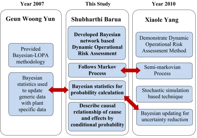
In figure 1, researches since 2007 done on dynamic operational risk assessment and Bayesian statistics at Mary Kay O’Connor Process Safety Center (MKOPSC) are described.

In 2007, Gen Woong Yun developed the Bayesian-LOPA methodology for performing risk assessment of a LNG importation terminal (Yun et al., 2009). This methodology employs Bayesian statistics to update general data obtained from databases with plant specific data. Generic data for equipment and component are obtained from several databases. LNG plant specific data are used for likelihood estimation and then combined with generic data to get posterior data.

In 2010, Xiaole Yang developed a dynamic operational risk assessment (DORA) methodology that follows semi-markovian approaches (Yang, 2010; Yang and Mannan, 2010). DORA methodology is mainly a stochastic simulation with the ability to quantify events. Component inspection and testing time interval is incorporated in the DORA method as a critical parameter. System state trajectory simulation is performed based on

Monte-Carlo method. The research also demonstrates application of Bayesian statistics for uncertainty reduction.

Figure 1. Researches on dynamic operational risk assessment and Bayesian statistics in MKOPSC

In this research, a new method for dynamic operational risk assessment method is demonstrated through applying the Bayesian network, an important subset of the Bayesian statistics. The methodology describes how conventional technique such as

Year 2010 Year 2007 This Study

Xiaole Yang

Bayesian updating for uncertainty reduction Stochastic simulation based technique

Shubharthi Barua

Bayesian statistics for probability calculation

Describe causal relationship of cause

and effects by conditional probability

Geun Woong Yun

Provided Bayesian-LOPA methodology Bayesian statistics used to update generic data with plant specific data

Fault tree, Event tree can be improved by mapping in the Bayesian network and demonstrates the dynamic Bayesian network’s ability to capture change in the values of different variables with time. The Bayesian statistics in previous researches are used to reduce uncertainty. In this study, by applying the Bayesian network, causal relationship between causes and effects are described by assigning conditional probability, and then the Bayesian statistics is used for probability estimation. Also, in previous studies, the Bayesian statistics is applied only for probability distribution, not for discrete values. This study has developed discrete time Bayesian network based dynamic operational risk assessment, and demonstrated the application of probability distribution for developing continuous-time Bayesian network based risk assessment method for future work.

1.5 Organization of This Thesis

Section 1 is an introductory chapter that provides background information, research scope and objectives. In Section 2, brief introduction on conventional risk assessment methodologies, previous researches on developing dynamic risk assessment techniques and Bayesian network’s application for reliability and risk analysis are discussed. The research methodology is presented in the following Section 3. In this chapter, overall research framework is explained. In Section 4, a case study is demonstrated to illustrate the application of developed method. In that chapter, an application of the developed method is provided to demonstrate the advantages of Bayesian network over other methods. In Section 5, an event tree generalization technique using Bayesian network is provided to illustrate parallelism with other

quantitative risk assessment techniques with Bayesian network. Section 6 provides overall summary and recommendations for future research.

2. LITERATURE REVIEW

2.1 General Background

The oil/gas, chemical, petrochemical and other process industries use equipment such as reactors, heat exchangers, distillation columns, storage vessels, pumps, compressors and complicated piping system. High level of heat and mass integration has made chemical process plant operation very complex and any small error can result catastrophic consequences. It is important to identify the hazards in the process and to know the risks posed by these hazards. Risk is a function of probability of any event occurrence and its consequence severity. Risk can be expressed as the measure of potential loss of property, human life, economic loss and other possible effects (Yang, 2010; Yang and Mannan, 2010). The risk assessment process identifies possible risks, characterizes their nature and magnitude, evaluates their occurrence probability, analyzes contributing factors, and assesses risk reduction measures. Risk analysis consists of risk assessment, risk management and risk communication (Yang, 2010; Yang and Mannan, 2010). The objective of performing risk assessment is to identify what can go wrong, how it can go wrong and its likelihood. Several qualitative and quantitative methods are available to perform risk analysis. The risk analysis method to be performed for a process is chosen depending on the scope of study required. This chapter provides brief introduction of the available risk analysis methodologies and demonstrates their limited ability of addressing different time-dependent effects of

dynamic process. Then a concise description of dynamic risk assessment methodologies, their strength and weakness are provided.

2.2 Conventional Risk Assessment Methodologies

A checklist is a methodical approach that lists all possible hazards or problems that may exist in a process industry. It is one of the simplest hazard identification methods (Khan and Abbasi, 1998). A checklist questions are mainly based on the operation and maintenance of a process plant, previous incident history, review of different documents, inspection and interview of plant personnel or based on standards and codes. A checklist development is dependent on the experiences of the personnel and it is very likely that some important aspects can be overlooked in a checklist. A checklist focuses on a single item at a time and has limited ability to detect hazards due to different operating condition in different equipment or unit operations. For these limitations, checklist application is limited.

What-if analysis is a systematic method that ask question starting with “what-if…” to identify potential irregularity in the process. It provides qualitative descriptions of any activity or system problem those results from human errors, abnormal process conditions equipment failures, etc. What-if analysis is especially useful for relatively simple failure scenarios.

A safety audit or review is done to detect safety problems in working zone i.e., process areas, laboratories etc. A safety review is conducted for new process or during modification of existing processes to identify any lacks in operating procedure or to

detect equipment conditions that may lead to an incident. The safety audit/review report provides insight into plant conditions from safety point of view and recommendations for improvements.

Hazard and Operability Study (HAZOP) is the most commonly used hazard identification methods. A multi-disciplinary team of experienced personnel from operations, maintenance and design review process flow diagrams, piping and instrumentation diagrams, process descriptions, operating procedures to identify possible consequences due to deviations from normal conditions and causes of deviations. HAZOP is based on different guidewords and provides primary ideas about hazards associated in a process with recommendations for minimizing or removing them. Like other qualitative methods, the quality of HAZOP is dependent on the experience of the people conducting it. The HAZOP procedure is briefly provided by Yang (2010). Khan and Abbasi (1998) described two main limitations of HAZOP, i.e., limited ability to incorporate spatial features with plant layout and requirement of long time to perform study.

The Norwegian Petroleum Directorate (NPD) was the first to make quantitative risk assessment mandatory for ‘Concept Safety Evaluation’ in their guideline published in 1981 (Norwegian Petroleum Directorate, 1981). But, it has received wide-spread acceptance in the oil and gas industry after the Piper Alpha disaster in 1988. The Lord Cullen investigation report (1990) on the Piper Alpha disaster recommended formulating quantitative risk assessment as an official requirement for the oil and gas industry. The U.K. Safety Case Regulation 1992 (UK HSE, 1992) made quantitative risk analysis

(QRA) mandatory for all existing and new installation in North Sea region. Since then, operators in the North Sea have to perform QRA studies to demonstrate that the potential risk is below the acceptable risk criteria and that actions have been taken to minimize the risk to ‘as low as reasonably practicable’. Vinnem (1998) summarized the application of quantitative risk assessment for offshore installations. Several quantitative risk assessment methods are described in this section briefly.

In 1961, Bell Telephone Laboratories developed the fault tree analysis (Khan and Abbasi, 1998). In 1975, the U.S. Nuclear Regulatory Commission introduced the fault tree for nuclear industry (The U.S. Nuclear Regulatory Commission, 1975). Later, the fault tree’s application has become extensive in reliability studies in the aerospace and chemical process industries. It is a graphical deductive process that starts reasoning from the top event to the undesirable events. In the conventional fault tree, there are two static gates, i.e. AND-gate, and OR-gate, that connect basic events failure with intermediate events and top event. In this approach, to understand failure mechanism explicitly, focus can be given to particular system failure at a time. But, the fault tree has some disadvantages as it can address common cause failures with limited ability (Khan and Abbasi, 1998). Fault tree has weakness in quantifying risks due to dynamically changing behavior or environment (Siu, 1994; Khan and Abbasi, 1998). Also, the conventional fault tree cannot adequately capture the sequential dependencies of equipment/components failure. Khan and Abbasi (1998) listed several studies that proposed improvement in conventional fault tree. Recently, Magott and Skrobanek (2012) proposed a fault tree based method which is capable of analyzing

time-dependencies. An event tree is an inductive process that demonstrates the sequences of different safeguards and human response failure due to an initiating event that lead to undesired consequences. The U.S. Nuclear Regulatory Commission (1975) introduced the method for nuclear industry and its application in chemical process industry is described by AIChE (2000), Mannan (2005), Delvosalle et al. (2006). Event tree’s application is advantageous to determine possible consequences probability due to different initiating event and subsequent safety barriers and protection failure.

The bow-tie method is a combination of an event tree and fault tree. It is a graphical representation of complete accident scenario in which fault tree provides different causes towards a critical event and the event tree describes possible consequences due to the critical event. Delvosalle et al. (2006) demonstrated Bow-tie method’s application for accident scenario identification in process industries. Mokhtari et al. (2011) proposed bow-tie based risk analysis method for sea ports and offshore terminals. Markowski and Kotynia (2011) demonstrated application of bow-tie model in layer of protection analysis (LOPA).

Layer of protection analysis (LOPA) is a semi-quantitative method that provides qualitative results of consequence with failure frequency data. It is derived from safety philosophy in the nuclear industry and became introduced to the process industry in the late nineties. The objective of performing layer of protection analysis is to determine sufficient independent safeguards that are available to prevent incidents. It should be noted all safeguards are not always independent layers of protection. Center for Chemical Process Safety (2001) described criteria for safeguards to be considered as

independent layer. Details of LOPA procedure are available at Center for Chemical Process Safety (2001), Markowshi A.S. (2006). Yun, G.W. (2007) incorporated Bayesian statistics to propose Bayesian-LOPA methodology for risk assessment.

2.3 Dynamic Risk Assessment Methods

Conventional risk assessment methods are static in nature. The oil/gas, chemical, petrochemical and other process industries are dynamic in nature. The process condition is dependent on variation of certain process variables which is affected by several time-dependent effects such as season changes, ageing of equipment/components, sequential dependencies, operator experiences and operation time, inspection and testing time interval etc. But, the conventional risk assessment methodologies have limited ability to quantify these time dependent effects. Siu (1994) summarized different methods developed for performing dynamic process systems risk assessment.

The Markov modeling is one of the widely accepted methods for dynamic risk analysis. State transition diagram is constructed to represent possible system states and transition from one state to another. A transition matrix is developed to characterize the Markov process. One of the limitations of the Markov process is that with increase of the system size, number of states also increases. It makes construction of system state transition diagram and computation complex (Reliability Analysis Center, 2003). Also, the Markov theory based models do not consider the effect of inspection on system-state transitions. The Markov model does not define the effect of inspection/testing time schedule.

Dynamic Logical Analytical Methodology (DYLAM) approach was proposed by Cacciabue et al. (1986). Nivolianitou et al. (1986) demonstrated application of DYLAM approach in reliability analysis of chemical processes. This method has the ability to quantify different time dependent effects by incorporating dynamic aspects of a process. It integrates physical behavior of the system and probabilistic modeling for analysis. In DYLAM, physical model for the system and component models for system components are constructed to predict system process variables reactions due to variations in component states. After defining undesired system states, the system model is simulated for all possible accident sequences to detect all possible combinations of status and states and calculate their likelihood. The DYLAM has limited ability to treat large number of scenarios and scenario calculations can be lengthier and more costly (Siu, 1994).

In the dynamic event tree, branching is allowed to take place at different points in time. Analyst defines the basis and required number of branches at any time step. Acosta and Siu (1993) described its application for accident sequence analysis.

Yang and Mannan (2010) proposed a semi-markovian approach named dynamic operational risk assessment (DORA) methodology. The DORA addresses dynamic effects in process industry by integrating process dynamic and system stochastic behavior. It can quantify risks for both component failure and component’s abnormal events. The DORA method incorporated inspection/testing time schedule to understand its effect on risk. Monte Carlo simulation is performed to understand system abnormal condition due to each individual component’s transition from one state to another and

then prolonged simulation is performed to understand effect of inspection and testing time on the probability of component abnormal event.

2.4 Overview of Bayesian Network Applications

Bayesian network is a probabilistic reasoning technique that can be very useful to represent complex dependencies between random variables. Weber et al. (2012) provides a summary of Bayesian network’s application in the field of dependability, risk analysis and maintenance. Application of Bayesian network for process safety, accident analysis and risk assessment is relatively new. As described in section 1.4, Khakzad et al. (2011) described Bayesian network application in accident analysis in the field of process safety based on the work by Bobbio et al. (2001) that demonstrated application of Bayesian network in improvement of dependable system. In the field of dependability, Boudali and Dugan (2005) demonstrated sequential dependencies of events and Montani et al. (2005) included temporal aspects for analyzing reliability analysis. Pasman and Rogers (2011) incorporated Bayesian network in layer of protection analysis. Hudson et al. (2002) described Bayesian network application on anti-terrorism risk management planning. Summary of similar studies in risk analysis is provided by Weber et al. (2012). Khakzad et al. (2012) mapped bow-tie method into Bayesian network. Any study in process safety and risk analysis is yet to conduct on temporal aspects. Using the temporal reasoning, dynamic risk assessment methodology can be provided by incorporating effects of time. This study uses temporal reasoning for

proposing a dynamic operational risk assessment methodology that can easily quantify operational changes due to sequential dependencies of equipment/components.

3. THE DEVELOPMENT OF BAYESIAN NETWORK BASED DYNAMIC OPERATIONAL RISK ASSESSMENT METHODOLOGY

In this section mapping procedure of conventional fault tree and dynamic fault tree in Bayesian network and then development dynamic operational risk assessment methodology based on Bayesian network is illustrated. This section demonstrates how to set up conditional probability tables for different dependent variables and Bayesian network ability to update prior probability with new information into posterior probability. This chapter provides brief introduction of fault tree, dynamic fault tree, Bayesian network and its characteristics and dynamic Bayesian network framework in section 3.1 and demonstrates the research framework with details of the mapping procedure in section 3.2.

3.1 Introduction

Bayesian network based dynamic operational risk assessment methodology, is a new technique developed in this research. This study demonstrates an advancement of application of Bayesian network in process safety. The methodology may provide more reliable description of different equipment or component failure probability with time for any oil/gas, chemical, petrochemical and other process industries. This method is very much helpful for those fields where availability of operational history is limited. In this section, brief description of fault tree, dynamic fault tree with characteristics and description of Bayesian network and dynamic Bayesian network is provided.

3.1.1 Dynamic fault tree

Conventional fault tree has limited ability to capture sequence dependencies in the system. If a system consists of a primary (active) pump and a back-up (standby) pump, then in case of primary pump failure, the back-up pump can become active and continues the system operation. But, if the back-up pump fails before the active pump fails, then the back-up pump fails to become active to substitute primary pump and the system is in failed state when the primary pump fails. Therefore, the failure criteria of the overall system are dependent on both the sequence and combinations of events. Dugan et al. (1990) defined different sequence dependencies and Dugan et al. (1992) introduced dynamic fault tree for fault tolerant computer systems. Dynamic fault tree goes over conventional fault tree by defining following dynamic gates which capture the component’s sequential and functional dependencies -

 The functional/probabilistic dependency gate (FDEP)/(PDEP)  The spare gates (Warm-WSP, Hot-HSP, Cold-CSP)

 The priority AND gate (PAND)  The sequence enforcing gate (SEQ)

This research work demonstrates development of dynamic fault tree using different dynamic gates introduced by Dugan et al. (1990, 1992). Brief descriptions of these gates are provided in this work.

3.1.1.1 The functional/probabilistic dependency gate (FDEP/PDEP)

In the functional dependency gate/probabilistic dependency gate, there is a trigger event on which some other events are dependent. The dependent events become

inaccessible in case of the trigger event occurrence. Figure 2 represents a function/probabilistic dependency gate. A trigger event can either be a basic event or output of another gate and its occurrence can cause two dependent events X and Y,

Figure 2. Functional/probabilistic dependency gate

inaccessible or unusable. Non-dependent output of the gate represents trigger event’s status.

3.1.1.2 The spare gates

A spare gate generally consists of a primary component/equipment that can be replaced with one or more standby similar component/equipment to perform the same function in case of its failure. Whenever primary equipment/component fails, then the first standby equipment/component becomes active to continue the operation. If the first

Trigger

X Y

FDEP/PDEP Status of the Trigger Event

standby fails, the next (if available) standby becomes active and so forth. A system with spare gate

Figure 3. Spare gates

fails, if primary and all standby equipment fails. Also, a standby component can fail while it is not active, but its individual failure has no effect on the overall system until the primary and other standby equipment/component can perform the function.

Figure 3, shows a spare gate, where a primary input has two standby input S1 and

S2. In case of primary input failure, at first S1 comes into operation and system continues

to function. If S1 fails, then S2 comes into operation and if S2 fails, then the system fails.

During Inactive state, the failure rate of the standby components/equipment is lower than that of in active state. Montani et al. (2005) defined dormancy factor, α, whose value can vary between 0 and 1, and stated that if the failure rate of a standby component is λ in

Gate Output

Primary S1 S2

active state, then its failure rate at inactive state is αλ. Spare gates are thus classified into three classes, i.e. Hot spare, Cold Spare and Warm Spare. If the standby component does not fail during inactive state, then it is called cold spare. But if the standby component fails during inactive state, then it is called hot spare. Different values of α, represents different spare gates. For, hot spare, α =1; for cold spare, α =0; and for warm spare, value of α is between 0 and 1. In figure 3, thus the standby input S1 and S2 may have

dormancy factor, α with any value between 0 and 1, and their failure during inactive state is lower than that of active state. Also, failure of this standby equipment when primary input is active, does not have any effect on the overall system.

3.1.1.3 The priority AND gate (PAND gate)

The priority AND-gate (PAND gate) consists of an AND-gate and pre-assigned order of inputs failure. In figure 4, two events X and Y are in a PAND gate and it is assigned that for the gate failure X has to fail before Y. Therefore, the output of the PAND gate in figure 4 is in failed state if both X and Y fails and X fails before Y. If Y fails before X, then PAND-gate output remains in normal state.

Figure 4. Probability AND-Gate (PAND gate)

3.1.1.4 The sequence enforcing gates (SEQ-gate)

In sequence enforcing gates, the inputs are constrained to fail in a particular order to cause system failure or a critical event to occur. The sequence enforcing gate fails only if its input failure occurs from left to right order. This is the difference between PAND-gate and SEQ-gate. Also, SEQ gates can be represented as spare gates. The difference is that spare gates have one or multiple standby input that can perform the same function as the primary input. But, in SEQ gates, the inputs can be any input performing different function.

3.1.2 Bayesian network

Bayesian network is widely applied in Artificial Intelligence (Pearl, 1988;

X Y

Neapolitan, 1990). Heckermann et al. (1995), Vomlel (2005) demonstrated some real life application of Bayesian network. Bobbio (2001) mapped fault trees into Bayesian network for dependability analysis and showed that Bayesian network has the ability to provide more precise reasoning with uncertainty. Recently, some authors applied Bayesian network in the field of process safety and accident modeling (Khakzad et al., 2011; Pasman and Rogers, 2011; Khakzad et al. 2012). Khakzad et al. (2011) demonstrated parallelism between fault tree and Bayesian network and described several advantages of Bayesian network’s application in the field of accident modeling and process safety. Pasman and Rogers (2011) incorporated Bayesian network to improve Layer of Protection Analysis. Khakzad et al. (2012) mapped bow-tie analysis in Bayesian network. Bayesian network’s application in the field of process safety and risk analysis is still relatively new and therefore, there is a scope for Bayesian network application for different study in this field.

A Bayesian network describes causal influence relations among variables via a directed acyclic graph. It represents a set of random variables in nodes and their conditional dependencies by drawing edges from one node to another. It has the ability to represent dependency among events clearly, accommodate multi- mode and continuous random variables, and incorporate information i.e. generic, system specific and expert judgment to support optimum decision making.

Figure 5. A simple Bayesian network

A simple Bayesian network is shown in figure 5. In a binary network, nodes and arcs represents variables and causal relationships among different nodes. Conditional probability tables or defined probabilistic relationships among nodes represent how one variable is linked another one or multi-variables. The nodes that influence other variables and have unconditional probability are called parent or root nodes. Nodes that are conditionally dependent on their direct parents are called intermediate nodes. The top node is defined as a leaf node.

Let be a Bayesian network, where, is a directed acyclic graph; V (random variables) represents nodes; and E represents edges between pairs of nodes of DAG. P represents probability distribution over V and can be either discrete or continuous random variables (Donohue and Dugan, 2003). These random variables are assigned to the nodes and the edges. Bayesian networks can be represented by the joint probability distribution P(V);

Here = parent nodes of Xi.

A main advantage of the application of Bayesian networks in risk analysis is the ability to update prior data using Bayes’ theorem by incorporating new information. Also, Bayesian networks have an advantage of handling different types of uncertainty. Bayesian network can be a very useful tool for the fields where availability of data is limited and in case one wants to exploit the scarce information available best.

3.1.3 Dynamic Bayesian network

A general Bayesian network is static in nature, i.e., the joint probability distribution is usually a representation of a fixed point or an interval of time (McNaught and Zagorecki, 2010). A dynamic Bayesian network describes the evolution of joint probability distribution over time and thus extends general Bayesian network. Discrete time modeling to represent the progression of time in dynamic Bayesian network was proposed by Dean and Kanazawa (1989). In a dynamic Bayesian network, arcs links nodes from previous time slice to that of the next time slice to represent temporal dependencies among them.

Montani et al. (2005) provided detailed mapping procedure of dynamic fault tree into dynamic Bayesian network in dependability analysis. Kjaerulff (1995) demonstrated that Markov assumption can be held true for dynamic Bayesian network if the variable state at future time slice ‘(n+1)-th’ time slice is independent of past given the present ‘n-th’ time slice. Boyen (1998) (Montani et al. 2005), Murphy (2002) described two-time slice Temporal Bayesian network.

3.1.4 Software

There are numbers of software available for developing and analyzing Bayesian network. Murphy (2007) provides a comparison among Bayesian network software. In this research, GeNIe 2.0, Bayesian network software developed by Decision Systems Laboratory (2010) is used for performing the analysis. This software is available free at http://genie.sis.pitt.edu/about.html and is compatible with other Bayesian network software. GeNIe supports both discrete and continuous variable though combination of both type of variables in a single network is still to be incorporated. GeNIe has temporal reasoning technique using which dynamic Bayesian network can be developed and analyzed. Other available software are: HUGIN (HUGIN EXPERT, 2012), BayesiaLab (BAYESIA SAS, 2010), Uninet (Lighttwist Software, 2008), BNT (Murphy,K., 2007) SAMIAM (AR Group-UCLA, 2010) etc.

3.2 Research Framework

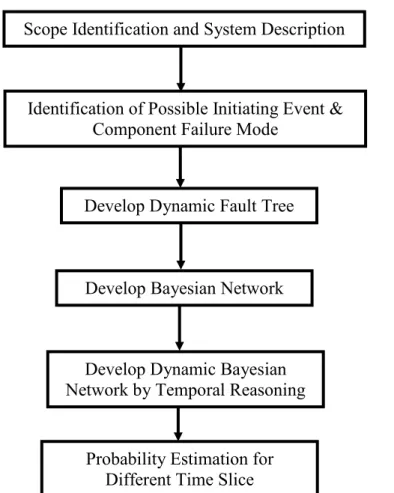
Figure 6 shows overall framework to development dynamic operational risk assessment with Bayesian network. This method has the ability to automatically update probability if failure rate data is provided at the first time slice and conditional dependency is given.

For developing dynamic operational risk assessment methodology based on Bayesian network, it is important to identify scope of work. It is also necessary to describe the system. According to the requirement, the scope can vary from small scale to large scale of system. For system description, process information as process block diagram, process flow diagram (PFD), piping and instrumentation diagram (P&ID), equipment/components in the system and their failure modes should be stated.

3.2.2 Identification of possible initiating event and component failure mode

The next step is to identify possible initiating event that can lead to accident. To identify possible initiating event, it is required to perform any hazards identification method which can be used to develop scenarios. Yang (2010) summarized qualitative hazard identification methods and process of conducting them. The next task is to identify different components failure modes that contribute to the occurrence of top event. In this step it is required to obtain failure rate data for different component. For this research, generic data are gathered from Center for Chemical Process Safety reliability data (AIChE 1989) and Offshore Reliability Data Handbook (SINTEF 2002).

It should be noted that generic data are historical data collected from similar industries and have limitation to properly reflect plant specific condition and characteristics of the plant equipment/component under consideration.

Figure 6. Framework for the dynamic Bayesian network based dynamic operational risk assessment method

3.2.3 Development of dynamic fault tree

Fault tree is a widely accepted method in oil/gas, chemical, petrochemical and other process plant for quantitative risk assessment. But, fault tree has limited capability to incorporate sequential dependencies. Therefore, this research proposes to develop dynamic fault tree for the system conceptually to capture sequential dependencies. Dynamic fault tree build-up is also a deductive process where top event is first identified

Scope Identification and System Description

Develop Dynamic Fault Tree

Develop Bayesian Network

Develop Dynamic Bayesian Network by Temporal Reasoning

Probability Estimation for Different Time Slice

Identification of Possible Initiating Event & Component Failure Mode

and then causes of that top event are detected. Sequential dependencies of different causes are identified and they are presented by dynamic gates as described in section 3.1.2. Events without sequential dependencies are presented by static fault tree gates. Detailed developing procedure of dynamic fault tree is described by Dugan et al. (1992).

3.2.4 Develop Bayesian network & dynamic Bayesian network

3.2.4.1 Bayesian network mapping

The next part is to map the dynamic fault tree into Bayesian network. Transforming dynamic fault tree in Bayesian network and eventually in dynamic Bayesian network is the important step for developing dynamic operational risk assessment with Bayesian network. The dynamic fault tree consists of two types of gates, i.e., the conventional fault tree gates and the dynamic gates. The conventional fault tree gates, i.e., OR-gate, AND-gate, K/M gates, involve equipment/component which does not show sequential dependencies. On the other hand, the dynamic gates i.e.,

spare gate, PAND gate, FDEP/PDEP gate and SEQ gate, describe sequential dependencies of different equipment/components.

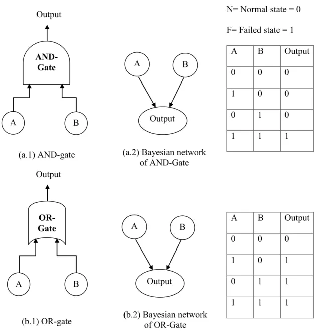
The static part of the dynamic fault tree is mapped in Bayesian network according to the method provided by Bobbio et al. (2001). The mapping algorithm consists of both graphical and quantitative transformation. For graphical mapping, all basic or primary events of fault tree root/parents nodes are created in the Bayesian network. Prior probability is calculated for the component using exponential distribution. Then, intermediate nodes and top event nodes are created for intermediate events and top event of the fault tree respectively. These event occurrences in Bayesian network are conditioned by assigning conditional probability table. In fault tree, the intermediate events are related to the basic or primary event through OR-gate and AND-gate. Figure 7 represents parallel Bayesian network for the OR-gate and AND-gate and their corresponding conditional probability table. Mapping of dynamic gates of dynamic fault tree are mainly based on Montani et al. (2005). Detailed description of different dynamic gates mapping in dynamic Bayesian network is discussed in section 3.2.4.2.

(a.1) AND-gate N= Normal state = 0 F= Failed state = 1 A B Output 0 0 0 1 0 0 0 1 0 1 1 1 (b.1) OR-gate A B Output 0 0 0 1 0 1 0 1 1 1 1 1

Figure 7. Mapping algorithm of AND-gate and OR-gate in Bayesian network

3.2.4.2 Dynamic Bayesian network development

The next step of the framework is to develop dynamic Bayesian network (DBN). In DBN, the nodes and their causal relationship are presented for various time slices.

A B Output A B Output AND-Gate A B Output OR-Gate A B Output

(a.2) Bayesian network of AND-Gate

(b.2) Bayesian network of OR-Gate

The important step in development of dynamic Bayesian network is to map dynamic gates of dynamic fault tree in dynamic Bayesian network. The mapping procedure of dynamic gates in this study is based on Montani et al. (2005) and is discussed in section 3.2.4.2.1. Then the network is expanded for different time slices as described in section 3.2.4.3.

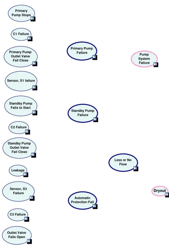
3.2.4.2.1 Mapping spare gate in Bayesian network

Figure 8 presents spare gates that has a primary component with two stand-by component S1 and S2 identical to the primary component. When primary component fails

then, the first stand-by S1 becomes active. If S1 fails, then S2 becomes active and keeps

the system operating. When primary and both stand-by S1 and S2 fail, then the warm

spare gates represent failed state of the system. These root nodes are provided with prior probability by using failure rate data in exponential distribution. Then this network is expanded for another time slice.

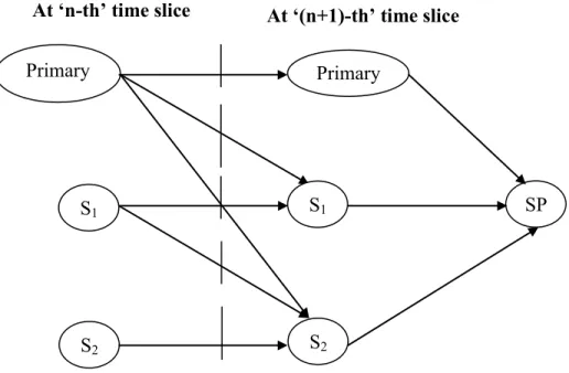
From figure 8, it is observed that each component node at next time slice is similar to that at the previous time slice. To represent the dependency of component state at different time-slices, an arc is drawn from primary component node, S1 node and S2

node of ‘n-th’ time slice to primary component node, S1 node and S2 node of ‘(n+1)-th’

time slice. It demonstrates that component states at ‘(n+1)-th’ time slice are dependent on their state at previous time slice. According to WSP, generally the primary component is in operation and if it fails, then the standby component becomes active. If the first standby component fails, then second standby component comes into operation.

The dependency is shown by drawing an arc from the primary component of ‘n-th’ slice to the stand-by components, S1 and S2 at ‘(n+1)-th’ time slice. Also, as second standby

component becomes active after first one’s failure, an arc is drawn from S1 of first

time-slice to S2 of next time slice. Therefore, if the primary component is active at first time

slice, then its failure rate will be λprimary and at that time standby component can fail with

failure rate αλS1 and αλS2. If primary component fails at ‘n-th time’ slice, then S1 is active

and it can fail at ‘(n+1)-th’ time slice with failure rate, λS1 and λS2 still have failure rate

equal to αλS2. The overall system become non-operational when primary and its entire

standby component fail.

Conditional probability table for components states in spare gates at ‘(n+1)-th’ time slice given the component state at ‘n-th’ time slice is provided in tables 1, 2 and 3. In tables 1 to 6, Δt represents interval between two time slices, i.e., ‘(n+1)-th’ and ‘n-th’ time slice. If ‘n-th’ time slice is at 3 months, and the ‘(n+1)-th’ time slice is at 6 months, then the time interval between the slices is,

Figure 8. Spare gates of dynamic fault tree mapping in dynamic Bayesian network (Montani et al., 2005)

Table 1 Conditional probability table for primary component state at ‘(n+1)-th’ time slice given its state at ‘n-th’ time slice

Primary Component State at ‘n-th’ Time Slice

Normal State Failed State State at

‘(n+1)-th’ Time Slice

Normal State Exp(-λprimary × Δt) 0

Failed State 1- Exp(-λprimary × Δt) 1

S2 SP Primary S1 S2 Primary S1

Table 2 Conditional probability table for the first standby component state at ‘(n+1)-th’ time slice given the state of primary component and first standby component at ‘n-th’ time slice

State at ‘n-th’ Time Slice

Primary Component Normal State Failed State

First Standby Component Normal State Failed

State Normal State

Failed State

State at ‘(n+1)-th’ Time Slice

Normal

State Exp(-αλS1Δt) 0 Exp(-λS1Δt) 0 Failed

Table 3 Conditional probability for second standby component state at ‘(n+1)-th’ time slice given state of primary component, first standby and second standby components state at ‘n-th’ time slice

State at ‘n-th’ Time Slice

Primary Normal Failed

First Standby Normal Failed Normal Failed

Second Standby Nor- mal Fai-led Nor- mal Fai-led Nor- mal Fai-led Nor- mal Fai-led At (n+1)-th Time Slice Nor mal Exp(-αλS2Δt) 0 Exp(-αλS2Δt) 0 Exp(-αλS2Δt) 0 Exp(-λS2Δt) 0 Faile d 1-Exp(-αλS2Δt) 1 1-Exp(-αλS2Δt) 1 1-Exp(-αλS2Δt) 1 1-Exp(-λS2Δt) 1

If any system consists of a primary component and ‘n’ number of standby components, then the n-th standby component will have 2n _{states in conditional}

probability table.

The conditional probability given in tables 1, 2 and 3 holds true if the primary and standby equipment failure in spare gate are basic events. However, if they are intermediate events as shown in figure 9, then it is required to incorporate conditional dependency of intermediate events on their respective basic events.

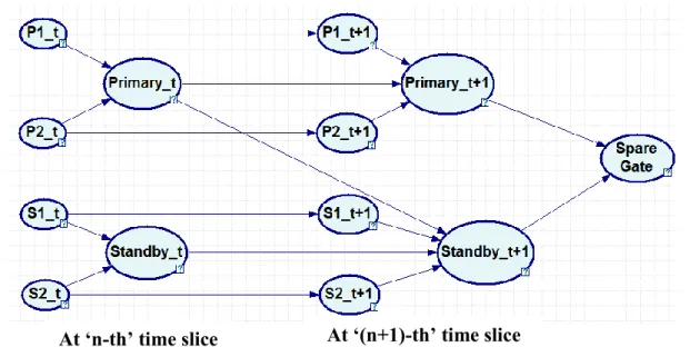
Figure 9. Spare gates of dynamic fault tree with intermediate inputs mapping in dynamic Bayesian network

If the basic events P1_t (failure rate, λP1_t) and P2_t (failure rate, λP2_t) are in an

OR-gate with the intermediate event Primary_t ((failure probability, λoverall) ) at n-th time

slice, then the overall failure rate of Primary_t at n-th time slice is the sum of basic events failure rate. If the basic event s P1_t (failure rate, λP1_t) and P2_t (failure rate,

λP2_t) are in an AND-gate with the intermediate event Primary_t ((failure probability,

λoverall) ) at n-th time slice, then the overall failure rate of Primary_t at n-th time slice is

the product of basic events failure rate. The above statements are also true for standby equipment. Therefore, the primary event node i.e. Primary_t+1 at (n+1)-th time slice is dependent on Primary_t of n-th time slice, P1_t+1 and P2_t+1 of (n+1)-th time slice. Similar dependency exists for standby_t+1 node. The conditional probability table for

primary and standby node at (n+1)-th time slice are given in tables 4 and 5.

Table 4 Conditional probability table for primary component state at ‘(n+1)-th’ time slice given its state at ‘n-th’ time slice for spare gate as in figure 9

Primary_t N F

P1_t+1 N F N F

P2_t+1 N F N F N F N F

Primary_t+1 N exp(-λoverall× Δt) 0 0 0 0 0 0 0 F 1- exp(-λoverall× Δt) 1 1 1 1 1 1 1

Table 5 Conditional probability table for standby component state at ‘(n+1)-th’ time slice given its state at ‘n-th’ time slice for spare gate as in figure 9

Primary_t N F Standby_t N F N F S1_t+1 N F N F N F N F S2_t+1 N F N F N F N F N F N F N F N F Primar y_t+1 N P1 0 0 0 0 0 0 0 P2 0 0 0 0 0 0 0 F 1-P1 1 1 1 1 1 1 1 1-P2 1 1 1 1 1 1 1

The value of P1 and P2 are as follows: P1= exp(-λoverall_standby × Δt)

P2= exp(-α × λoverall_standby × Δt)

3.2.4.2.2 Mapping functional/probabilistic dependency gate in Bayesian network

In function/probabilistic dependency gate (FDEP/PDEP), the status of the trigger event readily determines the states of the dependent event. The mapping procedure of FDEP/PDEP is based on work by Montani et al. (2005).

Figure 10. FDEP/PDEP gate mapping in dynamic Bayesian network (Montani et al., 2005)

At ‘n-th’ time slice At ‘(n+1)-th’ time slice

Trigger Event X Y X Y Trigger Event

In FDEP/PDEP gates, an arc connects the trigger event node at ‘n-th time slice’ with that node at the ‘(n+1)-th’ time slice. The dependent components, X and Y, on trigger event also have an arc from present to future time slice. Also, the trigger event has two arcs connected to the dependent components representing that the status of trigger event at a time-slice has impact on the dependent components. Detailed conditional probability table for FDEP/PDEP gate is provided in tables 6 and 7.

Table 6 Conditional probability table for trigger event at ‘(n+1)-th’ time slice given its state at ‘n-th’ time slice

Trigger Event State at ‘n-th’ Time Slice

Normal State Failed State State at ‘(n+1)-th’ Time

Slice

Normal State Exp(-λT × Δt) 0

Failed State 1- Exp(-λT × Δt) 1

Here, ‘λT’ represents the failure rate data of the trigger event and Δt gives the

Table 7 Conditional probability table for dependent components at ‘(n+1)-th’ time slice given the state of trigger event at ‘n-th’ time slice

State Trigger Event and Dependent Component at ‘n-th’ Time Slice

Trigger Event Normal State Failed State

State of Component at

‘(n+1)-th’ Time Slice Normal State

Failed

State Normal State

Failed State First Dependent Component, X Normal State Exp(-λXΔt) 0 0 0 Failed State 1-Exp(-λXΔt) 1 1 1 Second Dependent Component, Y Normal State Exp(-λYΔt) 0 0 0 Failed State 1-Exp(-λYΔt) 1 1 1

The structure of conditional probability tables for all dependent components is same. Hence, if the system has more dependent components than shown above, they will also have a similar conditional probability table.

3.2.4.2.3 Mapping priority AND-gate (PAND Gate)

The priority AND-gates require failure of all components in a pre-assigned order. Following are the conditional probability tables for the PAND-gate shown in figure 4, in which there are two components X and Y respectively and PAND-gate fails if X fails before Y fails.

Table 8 Conditional probability table for component ‘X’ at ‘(n+1)-th’ time slice given its state at ‘n-th’ time slice

Component ‘X’ State at ‘n-th’ Time Slice

Normal State Failed State State at ‘(n+1)-th’

Time Slice

Normal State Exp(-λX × Δt) 0

Failed State 1- Exp(-λX × Δt) 1

According to Montani et al. (2005) component Y can stay in operating or failed state before component X fails or failed after component X state fails. PAND gate will result in failure only if component X and component Y both fail and X fails before Y. Therefore, the values to put in conditional probability tables for component Y are given below: