Exploiting the structure of feature spaces in kernel learning

Exploiting the structure of feature spaces

in kernel learning

PhD student: Michele Donini

Advisor: Fabio Aiolli

Doctoral School in Mathematical Sciences

Computer Science area, XXVIII course

Sede Amministrativa: Università degli Studi di Padova Dipartimento di Matematica

___________________________________________________________________

SCUOLA DI DOTTORATO DI RICERCA IN: SCIENZE MATEMATICHE INDIRIZZO: INFORMATICA

CICLO: XXVIII

EXPLOITING THE STRUCTURE OF FEATURE SPACES IN KERNEL LEARNING

Direttore della Scuola: Ch.mo Prof. Pierpaolo Soravia

Coordinatore d’indirizzo: Ch.mo Prof. Francesca Rossi

Supervisore: Ch.mo Prof. Fabio Aiolli

Dottorando: Michele Donini

Contents

Riassunto

Abstract

I

Introduction & Background

1

Introduction

1.1 The Representation Problem 16

1.2 Aim and original contributions of this thesis 20

1.2.1 Structure of the thesis . . . 22

1.3 Publications 23

1.3.1 Journals . . . 23 1.3.2 Conferences . . . 23

2

Notation

2.1 Binary Classification Problem 25

2.1.1 Quality measures for binary classifications . . . 27 2.1.2 Datasets for Binary Vectorial Classification . . . 28

2.2 Graphs 30

2.2.1 Datasets . . . 32

3

Topics

3.1 Explicit and Implicit Feature Learning 33

3.1.1 Kernel Learning . . . 34 3.1.2 Metric Learning . . . 35 3.1.3 Feature Learning . . . 35

3.2 Explicit Feature Learning 36

3.2.1 Feature Selection methods . . . 36 3.2.2 Distance Metric Learning . . . 38

3.3 Implicit Feature Learning 40

3.3.1 Transductive Feature Extraction with Non Linear Kernels . 40 3.3.2 Spectral Kernel Learning . . . 40 3.3.3 Multiple Kernel Learning (MKL) . . . 41

4

Graph Kernels

4.1 An introduction to Graph kernels 48

4.1.1 Ordered Decomposition DAG Kernels for Graphs . . . 48 4.1.2 ODD kernels and feature weighting . . . 50

5

Optimization of the Margin Distribution

5.1 Playing with the margin 53

6

Rademacher Complexity

6.1 The expressiveness of a class of functions 57

6.1.1 Local Rademacher complexity . . . 59

II

A new approach to Multiple Kernel Learning

7

EasyMKL

7.1 A new scalable MKL algorithm 68

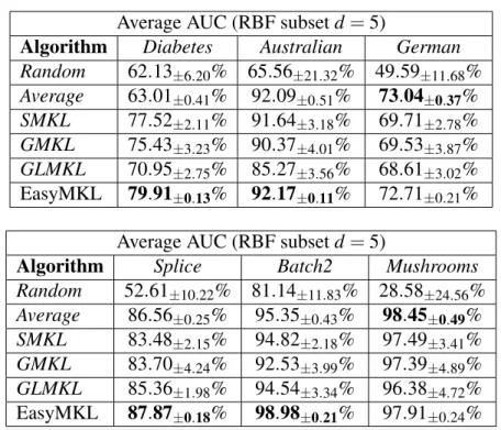
7.2 Experiments and Results 70

7.2.1 Experimental setting . . . 70 7.2.2 Is data separation a good criterion to maximize? . . . 71

7.2.3 Methods . . . 72

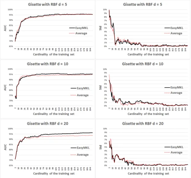
7.2.4 AUC comparisons . . . 73

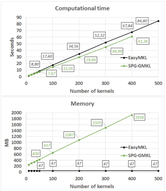
7.2.5 Performance in time and memory . . . 74

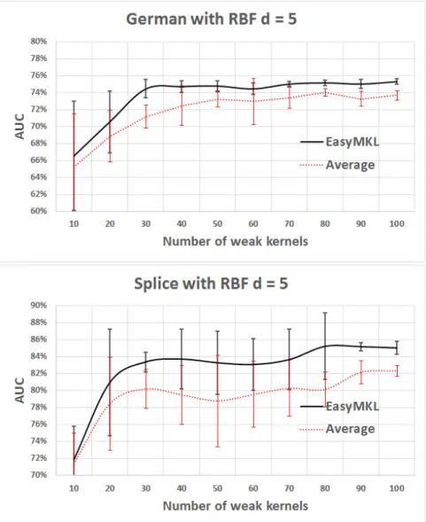
7.2.6 Stability with noisy features . . . 76

7.2.7 Performance changing the number ofweak kernels . . . . 80

7.3 Summary of the results 81

8

Spectral Complexity

8.1 A good measure for kernel complexity 83 8.2 Eigenvalues and Data Separation 84 8.3 A new measure for kernel complexity 85 8.3.1 A toy example using the RBF kernel . . . 87

8.4 Connection to the Rademacher complexity 88

9

Weak

kernels optimization

9.1 Dot-product Polynomial Kernels 92 9.2 MKL for learning the DPP coefficients 93 9.3 Exploiting the structure of the features 94 9.3.1 Margin and Complexity: an example . . . 94

9.4 Experimental Work 97 9.4.1 MKL for learning DPP . . . 97

9.4.2 Is the HPK structure important? . . . 98

9.4.3 A comparison with the Generalized Hierarchical Kernel Learn-ing . . . 107

9.5 Weak kernels on the ODD Graph-Kernel 107 9.5.1 Generating the weak kernels . . . 108

9.6 Experiments 111 9.6.1 Results . . . 112

9.7 Summary of the results 113

10

Learning the Anisotropic RBF

10.1 Connection between MKL and DML 115 10.2 Extending the game to features 116 10.2.1 Gradient based optimization forP_βββ . . . 118

10.2.3 Reducing the problemP_βββ to an unconstrained optimization

problem . . . 120

10.3 Experiments and Results 120

III

Real World Applications

11

MRI Segmentation

11.1 Motivation and importance of the MRI Segmentation 127 11.2 Material 128 11.2.1 Feature Extraction . . . 128

11.2.2 Classification . . . 131

11.2.3 Experimental Setting . . . 132

11.3 Results 132 11.4 Discussion and Conclusion 133

12

Climb the world

12.1 Motivation 135 12.2 Pipeline overview 136 12.3 Data smoothing 138 12.4 Data standardization 140 12.5 Segmentation with data-dependent window 142 12.6 Representation and features standardization 143 12.7 Experiments and results 145 12.7.1 Classification setting and results . . . 145

12.7.2 Energy consumption results . . . 147

12.7.3 Irrelevant features . . . 149

13

Distributed Variance Regularized MTL

13.1 The importance of the Multitask Learning 153 13.2 Multitask Learning Framework 155 13.3 Distributed MTL via ADMM 156 13.4 Algorithm 158 13.4.1 Optimization of each individual task . . . 158

13.4.3 Convergence . . . 160

13.5 SGD Optimization of each individual task 161

13.6 Experimental results 164 13.6.1 Artificial data . . . 164 13.6.2 URL classification . . . 167

IV

Conclusions

14

Conclusions

15

Future work

Bibliography

Riassunto

Il problema dell’apprendimento della reppresentazione ottima per un task specifico è divenuto un importante argomento nella comunità dell’apprendimento automatico.

In questo campo, le architetture di tipo deep sono attualmente le più avanzate tra i possibili algoritmi di apprendimento automatico. Esse generano modelli che utilizzando alti gradi di astrazione e sono in grado di scoprire strutture complicate in dataset anche molto ampi. I kernel e le Deep Neural Network (DNN) sono i principali metodi per apprendere una rappresentazione di un problema in modo ricco (cioè deep).

Le DNN sfruttano il famoso algoritmo di back-propagation migliorando le prestazioni degli algoritmi allo stato dell’arte in diverse applicazioni reali, come per esempio il riconoscimento vocale, il riconoscimento di oggetti o l’elaborazione di segnali.

Tuttavia, gli algoritmi DNN hanno anche delle problematiche, ereditate dalle classiche reti neurali e derivanti dal fatto che esse non sono completamente comprese teoricamente. I problemi principali sono: la complessità della struttura della soluzione, la non chiara separazione tra la fase di apprendimento della rappresentazione ottimale e del modello, i lunghi tempi di training e la convergenza a soluzioni ottime solo localmente (a causa dei minimi locali e del vanishing gradient).

Per questi motivi, in questa tesi, proponiamo nuove idee per ottenere rapprensetazioni ottimali sfruttando la teoria dei kernel. I metodi kernel hanno un elegante framework che separa l’algoritmo di apprendimento dalla rappresentazione delle informazioni. D’altro canto, anche i kernel hanno alcune debolezze, per esempio essi non scalano e, per come sono solitamente utilizzati, portano con loro una rappresentazione poco ricca (shallow).

10

In questa tesi, proponiamo nuovi risultati teorici e nuovi algoritmi per cercare di risolvere questi problemi e rendere l’apprendimento dei kernel in grado di generare rappre-sentazioni più ricche (deeper) ed essere più scalabili.

Verrà quindi presentato un nuovo algoritmo in grado di combinare migliaia di kernel deboli con un basso costo computazionale e di memoria. Questa procedura, chiamata EasyMKL, supera i metodi attualmente allo stato dell’arte combinando frammenti di informazione e creando in questo modo il kernel ottimale per uno specifico task.

Perseguendo l’idea di creare una famiglia di kernel deboli ottimale, abbiamo creato una nuova misura di valutazione dell’espressività dei kernel, chiamata Spectral Complexity. Sfruttando questa misura siamo in grado di generare famiglia di kernel deboli con una struttura gerarchica nelle feature definendo una nuova proprietà riguardante la monotonicità della Spectral Complexity.

Mostriamo la qualità dei nostri kernel deboli sviluppando una nuova metologia per il Multiple Kernel Learning (MKL). In primo luogo, siamo in grado di creare una famiglia ottimale di kernel deboli sfruttando la proprietà di monotinicità della Spectral Complexity; combiniamo quindi la famiglia di kernel deboli ottimale sfruttando EasyMKL e ottenendo un nuovo kernel, specifico per il singolo task; infine, siamo in grado di generare un modello sfruttando il nuovo kernel e kernel machine (per esempio una SVM).

Inoltre, in questa tesi sottolineiamo le connessioni tra Distance Metric Learning, Feature Larning e Kernel Learning proponendo un metodo per apprendere la famiglia ottimale di kernel deboli per un algoritmo MKL in un contesto differente, in cui la regola di combinazione è il prodotto componente per componente delle matrici kernel. Questo algoritmo è in grado di generare i parametri ottimali per un kernel RBF anisotropico. Di conseguenza, si crea un naturale collegamento tra il Feature Weighting, le combinazioni dei kernel e l’apprendimento della metrica ottimale per il task.

Infine, l’importanza della rappresentazione è anche presa in considerazione in tre task reali, dove affrontiamo differenti problematiche, tra cui: il rumore nei dati, le applicazioni in tempo reale e le grandi moli di dati (Big Data).

Abstract

The problem of learning the optimal representation for a specific task recently became an important and not trivial topic in the machine learning community.

In this field, deep architectures are the current gold standard among the machine learning algorithms by generating models with several levels of abstraction discovering very complicated structures in large datasets. Kernels and Deep Neural Networks (DNNs) are the principal methods to handle the representation problem in a deep manner.

A DNN uses the famous back-propagation algorithm improving the state-of-the-art performance in several different real world applications, e.g. speech recognition, object detection and signal processing.

Nevertheless, DNN algorithms have some drawbacks, inherited from standard neural networks, since they are theoretically not well understood. The main problems are: the complex structure of the solution, the unclear decoupling between the representation learning phase and the model generation, long training time, and the convergence to a sub-optimal solution (because of local minima and vanishing gradient).

For these reasons, in this thesis, we propose new ideas to obtain an optimal represen-tation by exploiting the kernels theory. Kernel methods have an elegant framework that decouples learning algorithms from data representations. On the other hand, kernels also have some weaknesses, for example they do not scale and they generally bring a shallow representation.

In this thesis, we propose new theory and algorithms to fill this gap and make kernel learning able to generate deeper representation and to be more scalable. An algorithm able

12

to combine thousands ofweakkernels with low computational and memory complexities is proposed. This procedure, called EasyMKL, outperforms the state-of-the-art methods combining the fragmented information in order to create an optimal kernel for the given task.

Pursuing the idea to create an optimal family ofweakkernels, we create a new measure for the evaluation of the kernel expressiveness, called spectral complexity. Exploiting this measure we are able to generate families of kernels with a hierarchical structure of the features by defining a new property concerning the monotonicity of the spectral complexity.

We prove the quality of theseweakfamilies of kernels developing a new methodology for the Multiple Kernel Learning (MKL). Firstly we are able to create an optimal family of

weakkernels by using the monotonically spectral-complex property; then we combine the optimal family of kernels by exploiting EasyMKL, obtaining a new kernel that is specific for the task; finally, we are able to generate the model by using a kernel machine.

Moreover, we highlight the connection among distance metric learning, feature learning and kernel learning by proposing a method to learn the optimal family ofweakkernels for a MKL algorithm in the different context in which the combination rule is the product element-wise of kernel matrices. This algorithm is able to generate the best parameters for an anisotropic RBF kernel and, therefore, a connection naturally appears among feature weighting, combinations of kernels and metric learning.

Finally, the importance of the representation is also taken into account in three tasks from real world problems where we tackle different issues such as noise data, real-time application and big data.

I

1

Introduction

1.1 The Representation Problem

1.2 Aim and original contributions of this thesis

1.3 Publications

2

Notation

2.1 Binary Classification Problem

2.2 Graphs

3

Topics

3.1 Explicit and Implicit Feature Learning 3.2 Explicit Feature Learning

3.3 Implicit Feature Learning

4

Graph Kernels

4.1 An introduction to Graph kernels

5

Optimization of the Margin

Distribu-tion

5.1 Playing with the margin

6

Rademacher Complexity

6.1 The expressiveness of a class of functions

1. Introduction

Machine learning’s purpose is to create algorithms able to optimize a performance criterion using examples from data or from past experience [8]. Given a model defined by some parameters, learning is the execution of a method to optimize them exploiting the training data. The model obtained should be able to make predictions in the future or to extract knowledge from data.

The theory of statistics is the most important tool exploited by machine learning in order to build mathematical models, since one of machine learning crucial tasks is making inference from a sample. Inference is the process of deriving logical conclusions from premises known, or assumed to be true (i.e. training examples). On the other hand, machine learning is more than only inference from a set of past experiences.

In fact, computer science is the second tool exploited by machine learning with two principal roles. Firstly, in training, where the efficiency of the algorithms is fundamental to solve the optimization problem and to store the solutions. Secondly, once we have a model, its representation and solution for inference needs to be efficient as well.

When we have to deal with a machine learning problem, the first step is to define a representation of the task, i.e. we have to select how to describe the known information. Typically, this pre-training step is performed to describe the problem that we have to solve in the best way possible by defining a set of features (explicitly or implicitly). In real world applications, the efficiency of the learning and the space and time complexity required by the methods have the same importance as to the predictive accuracy of the model.

16 Chapter 1. Introduction

from the introduction of the tackled problem.

1.1

The Representation Problem

The data representation plays a key role in the success of machine learning methods. Due to the current data growth in size, heterogeneity and structure, the new generation of algorithms are expected to solve increasingly challenging problems. This must be done under growing constraints such as computational resources, memory budget and energy consumption. The representation should ideally distill the relevant information about a learning problem in a compact manner, such that it becomes possible to learn the model from a small number of examples.

In the past, the research community has been focused on investigating new algorithms to obtain a model from a fixed apriorirepresentation. In fact, the learning process was considered mainly the process of choosing an appropriate function from a given set of functions [188].

A new point of view is arising in this last decade, and the problem of learning the optimal representation has become a hot topic in the most important conferences and journals. When dealing with the representation of a task, a plethora of questions arise. Some questions are simple to be formulated but the answers are not easy to be found. The first questions are: how can we find automatically a good representation for a specific task? How can we compare two representations to assert that one is better than another?

The research community has addressed the representation of a task by injecting some reasonable priors in general-purpose fashion. Examples of these injected priors are several, the most commonly used has been described by Bengio et al. in [28]:

• Smoothness: the assumption that the model to be learned can be described by a

smoothfunction f, i.e. if two examplesxandyare similar (x≈y) then the model has to produce similar outputs: f(x)≈ f(y);

• Multiple explanatory factors: the idea that a single factor can not describe the model and the underlying factors of variation have to be recovered (i.e the idea of the distributed representations);

• Hierarchical organization of the explanatory factors: the concept of a hierarchi-cal organization of data with moreabstractconcepts higher in the hierarchy;

• Shared factors across tasks: the existence of shared factors among the tasks (e.g. Multitask learning, Transfer Learning);

• Manifolds: the assumption that a task can be represented using a manifold of smaller dimensionality than the original representation;

• Sparsity: the idea that only a small fraction of all the possible factors is really relevant.

1.1 The Representation Problem 17

Finally, the main assumption is that if we are able to use an optimal representation, all the explanatory factors can be related using simple (e.g. linear) models.

The most ingenuous way to take advantage of a good representation for a specific (not general-purpose) task is the simple feature engineering. Anexpertof the task has to create a set of featuresad hocin order to solve the problem at the best of his knowledge. This approach is time consuming, sub-optimal and it contains a strong bias derived from the personal experience of the expert. However, in some real world applications, where the task to tackle is well understood, this methodology is currently applied with good results [102, 167].

Problems exist where we are not able to exploit the knowledge of an expert, nor to create specific features for a single task. For example, when dealing with speech recognition our brain does operations that we are not able to describe and it is not possible to create features of phenomena that we do not understand in depth.

In this context, a new branch of algorithms became famous in the last years, called

deep learning algorithms [125]. Deep learning generates models that are composed by a sequence of layers to learn representations of data with several levels of abstraction. The gold standard algorithms in the deep learning framework are represented by the Deep Neural Networks (DNNs). The DNNs are able to discover very complicated structures in large datasets by exploiting the back-propagation algorithm. These methods have changed the perspective in the machine learning community and improved the state-of-the-art in several different fields of application (e.g. speech recognition, visual object recognition, object detection and many others). Moreover, the deep convolutional neural networks have dramatically increased the performance of the machine learning algorithms when dealing with the processing of images, video, audio, text and speech (i.e. sequential or space-temporal data).

However, the biggest problem with deep learning is the very complex structure of the solution that imposes the utilization of the results as a sort ofblack box. Also, the convergence to the optimal solution is not theoretically guaranteed in these algorithms, and they suffer the same problems the standardneural networks[162, 67, 29, 135, 183, 209, 92, 146, 94, 93, 124]:

• They are theoretically not well understood;

• There is not a clear decoupling between the representation and the model generation;

• They have a high training time (more than 10 layers are difficult to be handled also using a non-common GPU cluster);

• They converge to a sub-optimal solution because of the local minima and the vanish-ing gradient issues;

18 Chapter 1. Introduction

issues.

A possible solution is to exploit the more solid theoretical framework concerning kernels. In a general spaceX, a kernel functionK:X×X→_Ris a positive semi-definite function and represents a dot product in an implicitly defined Hilbert space X (a.k.a., feature space). K represents a similarity measure between the elements in X. Given a kernelK, its feature mapping is a (typically non linear) embeddingφφφ :X→X. The kernel

Kcan be written in the form:

K(x,y) =φφφ(x)·φφφ(y), ∀x,y∈X. (1.1)

So, given a kernel, the explicit evaluation of the vector φφφ(x)is avoidable and we are able

to obtain a significant improvement in the performance of the kernel methods.

In the past, kernels have consistently outperformed previous generations of learning techniques because they provided a flexible and expressive learning framework that has been successfully applied to a wide range of real world problems. For example, kernel methods are widely applied in machine learning for structured data because, unlike the majority of machine learning techniques, their application to any type of data is painless as long as a kernel function for such data is defined. Kernel methods offer an elegant framework that decouples learning algorithms from data representations. On the other hand, kernels have lost some of their initial appealing in the research community, due to some of their weaknesses:

• The scaling problem and the high computational complexity: dealing with kernel based methods imposes the storage in memory of a kernel matrix, i.e. a matrix with a number of entries quadratic with respect to the number of examples. So, kernel methods are not able (in general) to tackle a task when the number of examples becomes huge;

• The shallowness of the representation: the representation implicitly defined by a shallow kernel does not take into account several layer of abstraction and is fixeda priori.

Moreover, the so called local kernels suffer thecurse of dimensionality [27], i.e. the problem of learning a model in a high dimensional space. This concept was coined by Bellman [25] and it refers to the exponential growth of hyper-volume as a function of dimensionality. Formally, we consider a local kernelKa kernel function with the following behavior:

lim

kx−xik2→+∞

K(x,xi) =Ci, (1.2)

wherexis a test example,xiis a training example andCiis a constant that does not depend

1.1 The Representation Problem 19

problem, as consequence of this behavior of the local kernels, the models generated by a kernel machine collapse to constant models (i.e. classifiers with the same output for all the examples) or to nearest neighbor models (i.e. the predicted class of an example is defined only by the nearest neighbor example in the high-dimensional space). In both cases, the obtained models have poor prediction (constant or highly local). Moreover, whenxis a high-dimensional vector, the nearest neighbor example is not much closer than the other examples, due to the geometrical properties of the high-dimensional spaces highlighted by Bellman.

New solutions have been recently presented with the aim to circumvent the difficulties concerning the scaling and the computational efficiency issues. For example, the random approximations of the kernels in order to avoid computational and memory issues are presented in [53, 174, 208]. These techniques consist in the approximation of the features of the Reproducing Kernel Hilbert Space (RKHS) to generate a linear kernel that approximates the original one. This new kernel can be used as a linear kernel in the original space and can be easily scaled-up. Using a linear kernel, the computational efficiency arises in a natural way exploiting the very efficient and distributed linear kernel machines (e.g. Pegasos [170]).

As pointed out before, the second critical issue about kernels is that they bring shallow and local information. In theory, kernels learn non-linear functionsφ in the input spaceX

and then they appear to be flexible as much as the DNN algorithms. However, traditionally, kernels were used to implement only a linear function in a pre-defined RKHS (the feature space). Starting from a fixeda priori kernel on a spaceX, the entire learning phase is performed in a single step by exploiting the implicit representationφφφK(x)of the examples

x∈X, as summarized in the following scheme:

x∈X→K_{f ixed}∼φφφK(x)→wlearned·φφφK(x).

Learning the weight vectorwimplicitly can been seen as a single layer learning and it is in contrast with the deep learning paradigm. In practice, theφφφK is fixeda prioriusing the

validation of the hyperparameters of the kernel (e.g. the parameterγ of the RBF kernel).

This methodology is not the best way to proceed if we are interested in finding the optimal representation because the fixed kernel is typically not the optimal kernel for a specific task.

Learning a new implicit representation defined by a kernel is one the current challenges in the machine learning research community. A theoretical connection between kernels and deep networks has already been highlighted in the past [142] building a sequence of deeper and deeper kernels that reproduce the mapping performed by more and more layers of the deep network and measuring how these increasingly complex kernels fit the learning

20 Chapter 1. Introduction

problem.

Kernel learning has the goal to learn the optimal kernel (and then the best implicit feature mapφ) given a specific task or set of tasks. Multiple Kernel Learning (MKL) [79]

is one of the most popular approach to kernel learning. MKL algorithms are designed to combine a set ofweak kernels to obtain a better one. MKL has the support of a theoretical framework [51] that claims a fundamental rule to overcome the shallowness of the single kernel representation. In particular, it has been proved that combining a large number of different kernels produces just a minor penalty in the generalization bounds. This result suggest that it is possible to combine thousands or millions of kernels without falling in the overfitting problem. A kernel can been seen as a different point of view of a task and then, the combination of millions of different point of views can be a solution to create a sort ofdeeper kernel, i.e. a kernel that is not shallow.

1.2

Aim and original contributions of this thesis

This thesis is focused on feature and kernel learning, aiming it improving the state-of-the-art on MKL and feature engineering in general. The original contribution of this thesis is four-fold:

1. Analysis of the MKL frameworkpursuing the idea of the deeper kernel. The problem of MKL is the computational complexity (in time and memory) and the creation of too shallow kernels. In Chapter 7, we propose a new algorithm able to combine thousands of kernels, called EasyMKL. A new scenario can be tackled in MKL where the weakkernels contain only a fragment of the information and the goal is to combine these fragments to obtain adeeperrepresentation. Exploiting this new methodology, we obtain a MKL algorithm that outperforms both the strong average baseline and the state-of-the-art MKL methods. Finally, EasyMKL also seems quite robust with respect to the noise introduced by features which are not informative and works well even when exploiting the classical MKL framework, with a small number ofweakkernels.

2. Study of the importance of the expressivenessof the family of weakkernels in order to inject a structure of expressiveness on them. MKL optimizes the margin among the examples and does not take into account the complexity of the combined kernels in theweakfamily. In this sense, a new technique is provided to measure the kernel complexity, called spectral complexity, in Chapter 8. This measure is easy to be evaluated and we exploit it to improve the MKL performance by creating optimalweakkernels families as a sort of pre-training of the data. Exploiting this measure, we define a new property of the weak families of kernels considering the monotonicity of the spectral complexity. This property imposes a hierarchical

1.2 Aim and original contributions of this thesis 21

structure among the features contained in differentweakkernels. We show that using these families, EasyMKL improves its results in term of AUC and we apply this methodology in two contexts: dot-product kernels, namely the kernels in the form

K(x,z) = f(x·z)and the ODD graph-kernel. In both cases, our approach improves the state-of-the-art results (see Chapter 9).

These results open a new scenario in MKL, that is beyond the combination of a large number ofweakkernels. Performing the creation of the correctweakfamily we are adding a third layer in the learning phase. In fact, this methodology have three steps:

(a) The first step is to create a good (and possibly large) family ofweakkernels starting from the raw information;

(b) Then, the second step is to combine all theweakkernels by exploiting MKL algorithms in order to fix the final representation;

(c) Finally, the last step is to create a model using a kernel machine. Practically, the methodology can be summarized as:

x∈X→ {K1, . . . ,KR}learned | {z } a →Klearned = R

∑

It is important to note that the first step of this procedure (x∈X→ {K1, . . . ,KR}learned)

is performed by considering only the hierarchical structure of the features, implicitly defined in the RKHS.

3. Connectionsof kernel learning, metric learning, feature learning and MKL. Study-ing the representation problem from different point of views, some of these connec-tions naturally arise, for example:

• Learning a metric to create new kernels or to perform explicit feature weighting;

• Using single feature kernels (i.e. 1−rank or 1−feature kernels) in a weak

family to connect MKL to the Group Lasso feature learning.

In Chapter 10, we study a new algorithm that is able to learn the hyperparameters of an Anisotropic RBF exploiting the connection among feature weighting, distance metric learning and MKL. This algorithm can also be seen as a MKL algorithm where the rule for the combination of theweakkernels is the entry-wise product of the weakmatrices. We consider eachweakkernel as a 1−feature RBF (i.e. RBF kernel that considers only 1 feature) and we optimize the parameters of these family of RBFs. Exploiting this methodology, we are able to create an optimal family of

weakkernels for this previously fixed MKL rule.

4. Real world tasks. The applicability of the new methods is widely important, not only on benchmark datasets. We prove our ideas in different real situations:

22 Chapter 1. Introduction

• In Chapter 11, a biomedical application will be presented, concerning the segmentation of brain MRI volumes. A new two-steps model is applied in order to exploit the domain knowledge ina priorimanner and using this model the different underlying factors of variation for this task are automatically highlighted improving the previous state-of-the-art results.

• In Chapter 12, an application for smartphone will be presented, calledClimb The World. The machine learning goal of this application is to count in real-time the number of stair-steps performed by a user by exploiting the sensors of the device. An extensive work of feature engineering and feature selection has been performed, using EasyMKL, to obtain optimal results under the constraints of battery consumption, imposed by the devices. The results achieved the goal of a very good real-time classification of the stairsteps and, at the best of our knowledge, this is the first algorithm that is able to solve this very difficult task.

• In Chapter 13, a new Multitask Learning (MTL) algorithm will be presented dealing with large scale datasets by using the alternating direction method of multipliers (ADMM). In the MTL context, this algorithm outperforms the previous state-of-the-art methods used in the classification of large scale dataset.

1.2.1 Structure of the thesis

This thesis is divided in four different parts. In Part I, the problem of representation in machine learning is presented. The principal notations are discussed in Chapter 2 and the state-of-the-art of the topics covered by this thesis are presented in Chapters 3, 4, 5 and 6.

In Part II, the original results of this thesis are depicted in four different chapters, concerning the creation of new algorithms to generate the optimal representation of a specific task:

• A new MKL algorithm is presented in Chapter 7. This algorithm is able to combine thousands of kernels using a fix amount of memory and with linear computation complexity and is calledEasyMKL;

• A new measure for kernel complexity is defined in Chapter 8, called spectral complexity. This new measure has a strict connection to theempirical Rademacher complexity;

• In Chapter 9, a new methodology is applied to generate good families ofweakkernels by exploiting the spectral complexityin two different cases. Firstly, in the space of the Dot-Product Polynomials (DPP) and then in the context of graph-kernels;

• In Chapter 10, a new algorithm is depicted that is able to learn the parameters of an Anisotropic Radial Basis Function (ARBF) kernel highlighting the connection

1.3 Publications 23

between metric learning, MKL and feature learning.

In Part III, three different real world applications are presented. In Chapter 11, a biomedical application about the segmentation of brain MRI volumes is presented. A new two-steps model is applied to exploit the domain knowledge ina priorimanner.

In Chapter 12, an applications for smartphone is presented, calledClimb The World. The learning task in this application was to count the number of stair-steps performed by a user by exploiting the sensors of the device. An extensive work of feature engineering and feature selection has been performed, using EasyMKL, to generate an optimal model under the constraints of battery consumption, imposed by the devices.

Finally, in Chapter 13, a new Multitask Learning (MTL) algorithm is presented that is able to deal with large scale datasets by using the Alternating Direction Method of Multipliers (ADMM).

In Part IV, conclusions and future work of this thesis are drawn.

1.3

Publications

A large part of this thesis has been presented in the following international peer-reviewed journals and conferences:

1.3.1 Journals

• (submitted) Increasing People Physical Activity using a Mobile Application.

Fabio Aiolli, Matteo Ciman, Michele Donini and Ombretta Gaggi. Pervasive and Mobile Computing 2015.

• EasyMKL: a scalable multiple kernel learning algorithm. Fabio Aiolli and Michele Donini. Neurocomputing 2015.

1.3.2 Conferences

• (submitted) Distributed Variance Regularized Multitask Learning. Michele Donini, David Martinez-Rego and Massimiliano Pontil. IJCNN 2016.

• (submitted)Learning the Kernel in the Space of Dot Product Polynomials.Michele Donini and Fabio Aiolli. ECML 2016.

• Advances in Learning with Kernels: Theory and Practice in a World of grow-ing Constraints. Luca Oneto, Nicolo Navarin, Michele Donini, Fabio Aiolli and

24 Chapter 1. Introduction

Davide Anguita. ESANN 2016.

• Measuring the Expressivity of Graph Kernels through the Rademacher Com-plexity. Luca Oneto, Nicolo Navarin, Michele Donini, Sperduti Alessandro, Fabio Aiolli and Davide Anguita.ESANN 2016.

• Multiple Graph-Kernel Learning. Fabio Aiolli, Michele Donini, Nicoló Navarin and Alessandro Sperduti. SSCI 2015.

• Feature and kernel learning. Verónica Bolón-Canedo, Michele Donini and Fabio Aiolli. ESANN 2015.

• ClimbTheWorld: Real-time stairstep counting to increase physical activity.

Fabio Aiolli, Matteo Ciman, Michele Donini and Ombretta Gaggi. MOBIQUI-TOUS 2014.

• Learning Anisotropic RBF Kernels. Fabio Aiolli and Michele Donini. ICANN 2014.

• Easy multiple kernel learning. Fabio Aiolli and Michele Donini. ESANN 2014.

• A Serious Game to persuade people to use stairs. Fabio Aiolli, Matteo Ciman, Michele Donini and Ombretta Gaggi. Persuasive 2014.

• Stacking Models for Efficient Annotation of Brain Tissues in MR Volumes.

2. Notation

In this chapter, we will introduce the main notations used in this thesis. The principal mathematical notations exploited in this thesis are presented in Table 2.1. In Section 2.1, the notations concerning the binary classification problem are depicted. Finally, in Section 2.2, the notations about graphs are introduced.

2.1

Binary Classification Problem

Considering the classification task, we define the training examples as{(xi,yi)}l_i=1, and

test examples as{(xi,yi)}L_i=l+1,xiin a generic setX,yiwith values+1 or−1. The matrix

K∈_RL×L_{is the complete kernel matrix containing the values of the kernel of each (training}

and test) data pair. Further, we indicate with an hat, like for example ˆy∈_Rlor ˆK∈_Rl×l, the submatrices (or subvectors) obtained considering training examples only.

Fixed a training set, ˆΓ will denote the domain of probability distributionsγγγ ∈_Rl₊

defined over the sets of positive and negative training examples: ˆ Γ={γγγ ∈Rl+ |

∑

∑

where ⊕ (resp. ) is the set of the indices of the positive examples (resp. negative examples). Note that any elementγγγ of the set ˆΓcorresponds to a pair of points, the first

in the convex hull of positive training examplesx+ =∑j∈⊕γjxj, and the second in the

26 Chapter 2. Notation

Symbol

M The bold capital letter are used to identify the matrices

M[i,j] The MatLab notation identifies the element in positioni,jof the matrixM M[:,j] The column jof the matrixM

M[i,:] The rowiof the matrixM

v The bold lower case letter are used to represent vectors

k · k1 The 1-norm of a matrix or a vector

k · k2 The 2-norm of a matrix or a vector

k · kF The Frobenious norm of a matrix

k · kT The Trace norm of a matrix

eig(M) The set of the eigenvalues of a matrix

1L A vector inRL where all the elements are equal to 1

I_L The identity matrix inRL×L

√

D The element-wise squared root of a matrixD

E The average of a variable Var The variance of a variable

sign(·) A functionR→ {−1,1}that returns 1 if the argument is positive,−1 otherwise

N

The element-wise product of vectors or matrices

∑ The element-wise summation of scalars, vectors or matrices

∏ The Capital Pi notation for a product of sequences of scalars, vectors or matrices

O The big O notation

a∝b The two quantitiesa,b∈_Rare proportional

2.1 Binary Classification Problem 27 R Usually, it is possible to consider the generic setXequal toRm. Then,X∈RL×m

denotes the matrix where examples are arranged in rows and ˆX∈Rl×mis the

sub-matrix obtained considering training examples only. In this case, theithexample is represented by theithrow ofX, namelyX[i,:].

2.1.1 Quality measures for binary classifications

Dealing with classification task, we are interested in finding which method has the best performance. The choice of an appropriate measure is very important to evaluate correctly the quality of a specific algorithm. The most important measures of quality are: accuracy, precision, recall, F_β and AUC1.

Accuracy

The accuracy of a model is the fraction of examples that are correctly classified using that model. It is a widely used metric for the performance of a classification algorithm. Despite the popularity of this measure, the accuracy suffers of some critical drawbacks:

• It assumes equal cost for both false positive and false negative errors;

• Thebase rateproblem: in the case of unbalanced dataset, a classifier that predicts constantly the predominant class could have a good accuracy;

• It does not consider the percent reduction in error (i.e. an improvement in accuracy of 0.1 from 0.8 to 0.9 is a reduction in error of 50%, on the other hand, an increase of accuracy of 0.01 from 0.99 to 1.0 is a reduction in error of 100%).

Precision, Recall and F_β

In a classification task, the precision for a class is the number of true positives (i.e. the number of items correctly labeled as belonging to the positive class) divided by the total number of elements labeled as belonging to the positive class (i.e. the sum of true positives and false positives, which are items incorrectly labeled as belonging to the class). Recall is defined as the number of true positives divided by the total number of elements that actually belong to the positive class (i.e. the sum of true positives and false negatives, which are items which were not labeled as belonging to the positive class but should have been).

The analytic formulas for these measures are: precision= T P

T P+FP

recall= T P T P+FN

whereT Pstands for True Positives,FPas False Positives andFN as False Negatives.

28 Chapter 2. Notation

F_β is a measure that consider a combination of precision and recall. This combination is weighted by a parameterβ ∈_R. The analytic formula of F_β is:

F_β = (1+β2) precision·recall β2precision+recall.

AUC

Solving a classification problem, the large part of the algorithms learn a model that is able to return a score value for each example. The union of all these scores can be seen as a ranking of the examples. The goal of a good model is to force the positive examples at the highest positions of the ranking. The Area Under Curve (AUC) is a metric that exploits the ranking given by the model.

Firstly, we have to define the Receiver Operating Characteristic (ROC) curve. The ROC curve is a graphical plot that illustrates the performance of a binary classifier system as its discrimination threshold is varied. The curve is created by plotting the true positive rate against the false positive rate at various threshold settings. The true-positive rate is also known as sensitivity or recall. The false-positive rate is also known as thef all−out

and can be calculated as: 1−specificity. The ROC curve is thus the sensitivity as a function of fall-out. The AUC is the (estimated) integral of the ROC Curve.

Given the prediction scores ofm examples, r∈_Rm_{, we can define analytically the}

Receiver Operating Characteristic Area Under Curvemetric (AUROC or AUC) as: AUC(r) = ∑

m

i=1ψ(xi)

2n_pn_n ∈[0,1], (2.2)

where we define np and nn as the number of positive and negative examples, and the

functionψ(xi)as:

ψ(xi) =|{xj:yj6=yi,rj<ri,j=1, . . . ,m}|ifyi=1, (2.3) ψ(xi) =|{xj:yj6=yi,rj>ri,j=1, . . . ,m}|ifyi=−1. (2.4)

The AUC represents the probability that a classifier will rank a randomly chosen positive instance higher than a randomly chosen negative one (assuming positive ranks higher than negative).

2.1.2 Datasets for Binary Vectorial Classification

In this section, we will present the 15 datasets used as benchmark in this thesis. These datasets are different for typology of the information, number and typology of the features and number of examples.

2.1 Binary Classification Problem 29 • Haberman: The dataset contains cases from a study that was conducted between 1958 and 1970 at the University of Chicago’s Billings Hospital on the survival of patients who had undergone surgery for breast cancer.

• Liver: This dataset is about BUPA liver disorders. The first 5 variables are all blood tests which are thought to be sensitive to liver disorders that might arise from excessive alcohol consumption.

• Diabetes: Diabetes patient records were obtained from two sources: an automatic electronic recording device and paper records. The automatic device had an internal clock to timestamp events, whereas the paper records only provided "logical time" slots (breakfast, lunch, dinner, bedtime). This dataset contain has been prepared for the use of participants for the 1994 AAAI Spring Symposium on Artificial Intelligence in Medicine.

• Abalone: Predicting the age of abalone from physical measurements. The age of abalone is determined by cutting the shell through the cone, staining it, and counting the number of rings through a microscope. Other measurements, which are easier to obtain, are used to predict the age. From the original data examples with missing values were removed.

• Australian: This file concerns credit card applications. All attribute names and values have been changed to meaningless symbols to protect confidentiality of the data. This dataset is interesting because there is a good mix of attributes: continuous, nominal with small numbers of values, and nominal with larger numbers of values.

• Pendigits: A digit database by collecting 250 samples from 44 writers. The authors used a WACOM PL-100V pressure sensitive tablet with an integrated LCD display and a cordless stylus. The tablet sendsxandytablet coordinates and pressure level values of the pen at fixed time intervals (sampling rate) of 100 milliseconds. These writers are asked to write 250 digits in random order inside boxes of 500 by 500 tablet pixel resolution. This dataset has been binarized for the classification problem ofeven vs. odd.

• Heart: This dataset is a heart disease database.

• German: This dataset classifies people described by a set of attributes as good or bad credit risks.

• Ionosphere: This dataset consists of a phased array of 16 high-frequency antennas with a total transmitted power on the order of 6.4 kilowatts. The targets were free electrons in the ionosphere. Received signals were processed using an autocorrela-tion funcautocorrela-tion whose arguments are the time of a pulse and the pulse number. There were 17 pulse numbers for the Goose Bay system. Instances in this database are described by 2 attributes per pulse number, corresponding to the complex values

30 Chapter 2. Notation

returned by the function resulting from the complex electromagnetic signal.

• Splice: Splice junctions are points on a DNA sequence at which superfluous DNA is removed during the process of protein creation in higher organisms. The problem posed in this dataset is to recognize, given a sequence of DNA, the boundaries between exons (the parts of the DNA sequence retained after splicing) and introns (the parts of the DNA sequence that are spliced out).

• Sonar: The task is to train a network to discriminate between sonar signals bounced off a metal cylinder and those bounced off a roughly cylindrical rock.

• Mush: This dataset includes descriptions of hypothetical samples corresponding to 23 species of gilled mushrooms in the Agaricus and Lepiota Family. Each species is identified as definitely edible, definitely poisonous, or of unknown edibility and not recommended. This dataset has been binarized.

• Batch2: This binarized dataset contains 1244 measurements from 16 chemical sensors exposed to 6 gases at different concentration levels. This dataset has been binarized.

• Colon: This dataset contains expression levels of 2000 genes taken in 62 different samples. For each sample it is indicated whether it came from a tumor biopsy or not.

• Gisette: This dataset is about a handwritten digit recognition problem. The problem is to separate the highly confusable digits ’4’ and ’9’. This dataset is one of five datasets of the NIPS 2003 feature selection challenge. A truncated version of this dataset, called GisetteT, is also used with a random sampling of 4000 examples from the original Gisette dataset.

Finally, in Table 2.2, the principal information about the datasets are summarized and in Table 2.3, the links to download the datasets are provided.

2.2

Graphs

In this section we summarize the principal notations about graphs used in this thesis (in Section 9.5) . Firstly, we can introduce a formal definition of a graphG:

Definition 2.2.1 A graphGcan be descried as tripletG= (VG,EG,LG)whereVGis the

set of vertices,E_Gthe set of edges andL_Ga function mapping nodes to labels.

Now, we are ready to define a list of the most used definitions and properties concerning graphs:

• A graph isundirectedif(vi,vj)∈EG⇔(vj,vi)∈EG, otherwise it isdirected.

• A path p(vi,vj)of lengthnin a graphGis a sequence of nodesv1, . . . ,vn, where

v₁=v_i,v_n=v_jand(vk,vk+1)∈EGfor 1≤k<n.

2.2 Graphs 31

Dataset Source Features Examples

Haberman UCI[18] 3 306 Liver UCI 6 345 Diabetes UCI 8 768 Abalone UCI 8 4177 Australian Statlog 14 690 Pendigits UCI 16 4000 Heart UCI 22 267 German Statlog 24 1000 Ionosphere UCI 34 351 Splice UCI 60 1000 Sonar UCI 60 208 Mush UCI 112 2000 Batch2[190] UCI 128 1244 Colon UCI 2000 62 GisetteT NIPS03 5000 4000 Gisette[82] NIPS03 5000 13500

Table 2.2: Datasets information: name, source, number of features and number of examples.

Dataset URL Haberman archive.ics.uci.edu/ml/datasets/Haberman's+Survival Liver archive.ics.uci.edu/ml/datasets/Liver+Disorders Diabetes archive.ics.uci.edu/ml/datasets/Diabetes Abalone archive.ics.uci.edu/ml/datasets/Abalone Australian www.csie.ntu.edu.tw/~cjlin/libsvmtools/datasets/binary/australian Pendigits archive.ics.uci.edu/ml/machine-learning-databases/pendigits/ Heart archive.ics.uci.edu/ml/datasets/Statlog+(Heart) German archive.ics.uci.edu/ml/datasets/Statlog+(German+Credit+Data) Ionosphere archive.ics.uci.edu/ml/datasets/Ionosphere Splice www.csie.ntu.edu.tw/~cjlin/libsvmtools/datasets/binary/splice_scale Sonar www.csie.ntu.edu.tw/~cjlin/libsvmtools/datasets/binary/sonar_scale Mush archive.ics.uci.edu/ml/datasets/Mushroom Batch2 archive.ics.uci.edu/ml/machine-learning-databases/00270/ Colon www.inf.ed.ac.uk/teaching/courses/dme/html/datasets0405.html Gisette archive.ics.uci.edu/ml/datasets/Gisette

32 Chapter 2. Notation

• A Directed Acyclic Graph (DAG) is a tree where each node has at most one incoming edge.

• Therootof a treeT is represented byr(T).

• The childrenof a nodev∈V_T are all the nodesv0s.t. (v,v0)∈E_T. ch_v[j]refers to the j-th child ofv.

• The maximum number of children in a tree is calledρ.

• Aproper subtreerooted at nodevcomprisesvand all its descendants.

2.2.1 Datasets

In this thesis, we compared different methods for the classification of structured data using five real-world graph datasets from bioinformatics: CAS2, CPDB [91], AIDS [198], NCI1 [194] and GDD [63]. The first four datasets represent chemical compounds: nodes represent atoms and are labeled according to the atom type, and edges represent bonds between atoms. GDD is a dataset of proteins. In this case, each node in a graph represents an amino acid and is labeled according to the amino acid type. In GDD, there is an edge connecting two nodes if the corresponding amino acids are less than 6 apart in the 3-dimensional folding of the protein. All the datasets encode binary classification problems.

3. Topics

Finding the best representation of the data has been an active research area in the last few decades obtaining success in many different applications. For example, with the advent of big data, the adequate identification of the relevant information has converted representation learning in an even more indispensable step. An important part of this thesis is concerning the representation given by feature and kernel learning.

In kernel methods, features are implicitly represented by means of feature mappings and kernels. It has been shown that the correct selection of the kernel is a crucial task, as long as an erroneous selection can lead to poor performance. Unfortunately, manually searching for an optimal kernel is a time-consuming and a sub-optimal choice.

This chapter is concerned with the background of the methods exploited in this thesis to learn automatically features, kernels and new representations from the data. Firstly, we can introduce a taxonomy of these methods in two families: Explicit Feature Learning

(EFL) andImplicit Feature Learning(IFL).

3.1

Explicit and Implicit Feature Learning

It is possible to divide the representation learning methods in two different families. In the first family are contained the methods where the features are learned explicitly in the original space. We call the methods in this family theExplicit Feature Learning(EFL) algorithms. EFL methods exploit the combination of the information contained in the data in an explicit way. They highlight clearly which features is more important than the others, and due to this particular behavior, the EFL methods are useful to identify the motivation

34 Chapter 3. Topics

behind the importance of the information. In real wold application, EFL methods have a widely success because of the simple interpretation of the results.

On the other hand, there are a plethora of methods that are, indirectly, able to exploit the information in the RKHS (or in a different non linear feature space). We can call this second family of methodsImplicit Feature Learning(IFL). This family contains methods that are more complex and sophisticated than the EFL methods. IFL becomes popular only few years ago and nowadays the research community is very active on this topic.

In the following sections, the topics covered by this thesis will be presented, starting from a brief overview of kernel learning, feature learning and metric learning. Finally, a deep analysis of the EFL and IFL families will be depicted, concerning the principal methods exploited in Part II and Part III.

3.1.1 Kernel Learning

Kernel machines and kernel-based algorithms are very popular in machine learning and have shown state-of-the-art performance. Kernel methods have been used to tackle a variety of learning tasks (e.g. classification, regression, clustering and more). In these algorithms the features are provided intrinsically using a positive semi-definite kernel function that can be interpreted as a similarity measure (i.e. a scalar product) in a high dimensional Hilbert space. The goal of Kernel Learning (KL) is to create methods able to provide automatically good kernels for a particular problem and avoiding, in this way, the arbitrary user’s choice of a kernel function. A bad choice of the kernel function can make learning very difficult because it corresponds to a sub-optimal choice of the features.

KL is often adopted within a semi-supervised learning setting [44, 212, 50, 130] and tries to learn the kernel matrix using all the available data (labeled and unlabeled examples) optimizing an objective function that improves the accordance between the kernel and the set of i.i.d. labeled data. Different ways have been investigated to obtain this result, e.g. maximizing the alignment [123, 52] or exploiting bounds on the(local) Rademacher complexity[48]. Conversely, unlabeled data are typically used to regularize the models avoiding the non-smoothness of the discriminant function.

Evaluation of the KL methods

The performance evaluation of a KL algorithm applied to a binary classification task can be computed by exploiting one of the several measures of quality, e.g, accuracy, precision, recall, F_β and more. In this thesis, the experimental evaluation of a kernel will be performed by using theReceiver Operating Characteristic Area Under Curvemetric (AUC). The AUC represents the probability that a classifier will rank a randomly chosen

positive instance higher than a randomly chosen negative one (assuming positive ranks higher than negative). We have chosen the AUC measure because we are able to avoid the

3.1 Explicit and Implicit Feature Learning 35

validation of the threshold parameter. This parameter is influenced by the kernel machine (i.e. the classifier) and not by (the quality) of the kernel.

3.1.2 Metric Learning

It is well known that different features typically have unequal impact and importance in solving a given classification task. This motivates several feature selection methods to select or weight different features in different ways. While feature selection is generally very difficult to perform with nonlinear kernels, one can learn the metric directly from data more easily [24]. This task is known as Distance Metric Learning (DML). For example, many researchers (see [75], [76], [169], [64]) have proposed a number of algorithms for the optimization of the Mahalanobis distance. Specifically, they replace the common Euclidean metric with the more powerful distance

(xi−xj)>M(xi−xj) (3.1)

and try to learn the combination matrixM. The learned distance is typically optimized for (and used in) a nearest neighbors setting. The high number of free parameters to learn together with the fact that these methods are used with nearest neighbors, make these approaches prone to overfitting, in particular when the training sample is small.

3.1.3 Feature Learning

In the last few years, several datasets with high dimensionality have become publicly available on the Internet. This fact has brought an interesting challenge to the research community, since for the machine learning methods it is difficult to deal with a high number of input features. To cope with the problem of the high number of input fea-tures, dimensionality reduction techniques can be applied to reduce the dimensionality of the original data and improve learning performance. These dimensionality reduction techniques usually come in two flavors:feature selectionandfeature extraction.

Feature selection and feature extraction each have their own merits [211]. On the one hand, feature extraction techniques achieve dimensionality reduction by combining the original features. In this manner, they are able to generate a set of new features, which is usually more compact and of stronger discriminating power. It is preferable in applications such as image analysis, signal processing, and information retrieval, where model accuracy is more important than model interpretability. On the other hand, feature selection achieves dimensionality reduction by removing the irrelevant and redundant features. It is widely used in data mining applications, such as text mining, genetics analysis, and sensor data processing. Due to the fact that feature selection maintains the original features, it is especially useful for applications where the original features are important for model

36 Chapter 3. Topics

interpretation and knowledge extraction.

Feature selection methods are usually divided into three major approaches based upon the relationship between a feature selection algorithm and the inductive learning method used to infer a model [81].Filtersrely on the general characteristics of training data and carry out the feature selection process as a pre-processing step independently from the induction algorithm. On the contrary,wrappersinvolve optimizing a predictor as a part of the selection process. In between them one can findembeddedmethods, which perform feature selection in the process of training and are usually specific to given learning machines. Popular and widely-used feature selection methods are Correlation-based Feature Selection (CFS) [86], minimum Redundancy Maximum Relevance (mRMR) [150], or Support Vector Machine - Recursive Feature Elimination (SVM-RFE) [83], among the others.

As for feature extraction, the most popular method is Principal Component Analysis (PCA) [109], which converts a set of observations of possibly correlated features into a set of values of linearly uncorrelated features called principal components. The number of principal components is less than or equal to the number of original features.

3.2

Explicit Feature Learning

3.2.1 Feature Selection methods

New feature selection methods have been steadily appearing during the last few decades. The proliferation of feature selection algorithms, however, has not brought about a general methodology that allows for intelligent selection from existing algorithms. Nevertheless, although a vast body of feature selection methods exists, some of them have been able to stand out and their use has become very popular among researchers. A brief description of them can be found in Table 3.1.

Filter/Embedded Ranker/Subset Reference Chi-Squared Filter Ranker Liu and Setiono [131] F-score (Fisher score) Filter Ranker Duda et al. [65] Information Gain Filter Ranker Quinlan [155] ReliefF Filter Ranker Kononenko [121] mRMR Filter Ranker Peng et al. [150] SVM-RFE Embedded Ranker Guyon et al. [83] CFS Filter Subset Hall [86] FCBF Filter Subset Yu and Liu [206] INTERACT Filter Subset Zhao and Liu [210] Consistency Filter Subset Dash and Liu [60]

3.2 Explicit Feature Learning 37

These methods are usually present in the review papers that appear in the literature for feature selection. In [161], classical feature selection techniques are provided in the form of a basic taxonomy and their applicability to bioinformatics applications is discussed. Another work on comparing state-of-the-art feature selection methods when dealing with thousands of features, using both synthetic data and real data, is presented in [98]. Brown et al. [38] presented a unifying framework for feature selection based on information theory, covering up to 17 different methods. More recently, the performance of well-known feature selection methods in the presence of several complications (such as noise, redundancy or interaction between attributes) was tested in [33].

Recent contributions

There exist numerous papers and books proving the benefits of the feature selection process [81]. In [161], classical feature selection techniques are provided in the form of a basic taxonomy and their applicability to bio-informatics applications is discussed. Another work on comparing state-of-the-art feature selection methods when dealing with thousands of features, using both synthetic data and real data, is presented in [98]. Brown et al. [38] presented a unifying framework for feature selection based on information theory, covering up to 17 different methods. More recently, the performance of well-known feature selection methods in the presence of several complications (such as noise, redundancy or interaction between attributes) was tested in [33].

However, since none of the existing methods mentioned has demonstrated significantly superiority over the others, researchers are usually focused on finding a good method for a specific problem setting. Therefore, new and novel feature selection methods are constantly appearing using different strategies. In the last few years, the review of the literature has shown a tendency to mix algorithms, either in the form of hybrid methods [187, 97, 126, 200] or ensemble methods [88, 203, 204, 114, 34].

Applications

Feature selection methods are currently being applied to problems of very different areas. In the next paragraphs we will describe some of the most popular applications that are promoting the use of feature selection:

• Computational biology. Bio-informatic tools have been widely applied to ge-nomics, proteomics, gene networks, structure prediction, disease diagnosis and drug design. DNA microarrays have been widely used in simultaneously monitoring mRNA expressions of thousands of genes in many areas of biomedical research. These data sets typically consist of several hundred samples as opposed to thousands of genes, whereby feature selection is paramount. Because of this, a myriad of works in the feature selection field have been devoted to help in the classification of DNA

38 Chapter 3. Topics

microarrays. A complete review of up-to-date feature selection methods developed for dealing with microarray data can be found in [32].

• Face recognition. The recognition of a human face has a wide range of applications, such as face-based video indexing and browsing engines, biometric identity authen-tication, human-computer interaction, and multimedia monitoring/surveillance. An important issue in this field is to determine which features from an image are the most informative for recognition purposes, so feature selection algorithms for face recognition have been recently suggested [129, 134, 9, 158, 137, 111]

• Health studies. The recent explosion in data available for analysis is as evident in health care as anywhere else. Private and public insurers, health care providers, particularly hospitals, physician groups and laboratories, and government agencies are able to generate far more digital information than ever before. Many health studies are longitudinal: each subject is followed over a period of time and many covariates and responses of each subject are collected at different time points. Feature selection has proven effective in helping with the diagnosis of several diseases, such as retinopathy of prematurity [12], evaporative dry eye [160], pulmonary nodules [127] or cardiac pacemaker implantation [103], among others.

• Financial engineering and risk management. Technological revolution and trade globalization have introduced a new era of financial markets. Over the last three decades, an enormous number of new financial products have been created to meet customer demands. The stock market trend is very complex and is influenced by various factors. Therefore it is very necessary to find out the most significant factors of the stock market and feature selection can be applied to achieve this goal [99, 116, 128, 186].

• Text classification. The categorization of documents into a fixed number of pre-defined categories has become a popular problem in Internet applications such as Spam email or shopping. Each unique word in a document is considered as a feature, so it is highly important to select a subset of all the possible features, allowing to reduce the computational requirements of learning algorithms. In the last few years, a number of works which promote the use of feature selection for text categorization have been presented [70, 115, 59, 71, 187].

3.2.2 Distance Metric Learning

Distance metric learning(DML) methods try to learn the best metric for a specific input space and dataset. The performance of a learning algorithm (nearest-neighbors classifiers, kernel algorithms etc.) mostly depends on the metric used. Many DML algorithms have been proposed. All of them try to find a positive semi-definite (PSD) matrixM∈_Rm×m

3.2 Explicit Feature Learning 39

such that the induced metric

d_M(xi,xj) = (xi−xj)>M(xi−xj) (3.2)

is optimal for the task at hand. For example, the Euclidian distance is a special case where

M=I. There are three principal families of DML algorithms [197]: eigenvector methods,

convex optimizationandneighborhood component analysis.

In the eigenvector methods, the matrixMis parameterized by the product of a real valued matrix with its transposed, namely M=L>L, in order to maintain the matrix positive semi-definite. In this case, the matrixMis called Mahalanobis metric. These methods use the covariance matrix to optimize the linear transformationxi→Lxi that

projects the training inputs. Finding the optimal projection is the task of eigenvector methods with a constraint that definesLas a projection matrix:LL>=I. These algorithms do not use the training labels and then they are totally unsupervised.

Convex optimization algorithms represent another family of DML algorithms. It is possible to formulate a DML as a convex optimization problem over the cone of correct matricesM. This cone is the cone of positive semi-definite matrices

M={M∈_Rm×m:∀τ ∈eig(M),τ ≥0}. (3.3)

Algorithms in this family are supervised and optimal positive semi-definite matrixMis obtained optimizing the square root of theMahalanobis metricand enforcing the SDP constraintM0. There are also online versions of convex optimization algorithms for DML, likePOLA[169] for example.

Another family of algorithms for DML is called neighborhood component analysis. In [76], for example, the authors try to learn a Mahalanobis metric from the expected leave-one-out classification error. In this case they use a stochastic variant ofk-nearest neighbor

withMahalanobis metric. This algorithm has an objective function that is not convex and can suffer from local minima. Metric Learning by Collapsing Classes (MLCC) [75] is an evolution of the above mentioned method that can be formulated by a convex problem but with the hypothesis that the examples in each class have only one mode. Another important algorithm in this family is the Large Margin Nearest Neighbor Classification (LMNNC) [197] that learns aMahalanobis distance metricwith ak-nearest neighbor by semi-definite programming and also in this case we have the semi-positive constraint for

M in the optimization problem. Finally, a generalization of the LMNNC is the Gradient Boosted LMNNC (GB-LMNNC) [113] that learns a non-linear transformation directly in the function space. Specifically, it extends theMahalanobis metricbetween two examples (e.g.:kLxi−Lxjk2) by using a non linear transformationφ to define the new Euclidian

40 Chapter 3. Topics

distancekφφφ(xi)−φφφ(xj)k2. Given the non linearity ofφφφ, GB-LMNNC uses the gradient

boosted regression tree in order to change the metric (GBRT) [72]. So, the algorithm learns and combines an ensemble of multivariate regression trees (that are weaklearners) using gradient boosting that minimizes the original LMNN objective function in the function space.

3.3

Implicit Feature Learning

3.3.1 Transductive Feature Extraction with Non Linear Kernels

Algorithms in this class of KL methods are able to perform feature extraction in the feature space defined by a non linear kernel. In this case, the feature mapping from the input space to the feature space is not explicitly defined. A popular solution is given by Kernel Principal Component Analysis(KPCA) [164]. KPCA uses thekernel trickto implicitly find the projections on the eigenvectors (principal directions) and the corresponding eigenvalues of the covariance matrix in feature space. KPCA can also be considered as an unsupervised manifold learning technique mapping data points into a lower-dimensional space.

The intrinsic problem of these algorithms is the transductive environment that they require (i.e. both training and test example needs to be available before training the classi-fier). This problem can be overcome by using Out-Of-Sample techniques to approximate the kernel values on new examples. Empirical experiments have shown that errors on examples in theOut-Of-Sampleset and examples in theIn-Sampleset are similar [30].

3.3.2 Spectral Kernel Learning

These methods are founded on the spectral decomposition of the Laplacian graphL, that is an undirected graph that contains the manifold structure of the data. By using these methods we are interested in finding the smoothest components ofL(i.e. the eigenvectors with the smaller eigenvalues) and hence building a kernel which penalizes large changes between strongly connected nodes. This can be made by changing the spectral representation of L

rescaling the eigenvalues in according to the semi-supervised information, for examples using linear programming [132]. More specifically, these algorithms are based on the possibility to write a semi-positive definite matrix L∈_Rl×l _{using the equation of its}

spectral decomposition: L= l

∑

{us}l_s=1,U is the matrix of the eigenvectors in rows and Dλλλ is a diagonal matrix with