A Thesis Submitted to the Faculty
of Drexel University
by Xiaoli Song in partial fulfillment of the requirements for the degree
of
Doctor of Philosophy December 2016
Acknowledgments
Thank God for giving me all the help, strength and determination to complete my thesis. I thank my advisor Dr. Xiaohua Hu. His guidance helped to shape and provided much needed focus to my work. I thank my dissertation committee members: Dr. Weimao Ke, Dr. Yuan An, Dr. Erjia Yan and Dr. Li Sheng for their support and insight throughout my research. I would also like to thank my fellow graduate students Zunyan Xiong, Jia Huang, Wanying Ding, Yue Shang, Mengwen Liu, Yuan Ling, Bo Song, and Yizhou Zang for all the help and support they provided. Special thanks to Chunyu Zhao, Yujia Wang, and Weilun Cheng.
Table of Contents
LIST OFTABLES . . . vii
LIST OFFIGURES. . . ix
ABSTRACT . . . x
1. INTRODUCTION. . . 1
1.1 Overview . . . 2
2. CLASSICALTOPICMODELINGMETHODS . . . 4
2.0.1 Latent Semantic Analysis (LSA) . . . 4
2.0.2 PLSA . . . 5
2.1 Latent Dirichlet Allocation . . . 6
3. PAIRWISETOPICMODEL . . . 8
3.1 Pairwise Relation Graph . . . 10
3.2 Problem Formulation . . . 10
4. PAIRWISETOPICMODELI . . . 12
4.1 Introduction . . . 12
4.2 Related Work . . . 13
4.3 Document Representation . . . 15
4.4 Pairwise Topic Model . . . 15
4.5 Model Description . . . 17 4.5.1 PTM-1 . . . 17 4.5.2 PTM-2 . . . 18 4.5.3 PTM-3 . . . 19 4.5.4 PTM-4 . . . 20 4.5.5 PTM-5 . . . 21 4.5.6 PTM-6 . . . 22
4.6 Inference . . . 24
4.6.1 Experiment . . . 26
4.7 Result and Evaluation . . . 27
4.7.1 Empirical Result . . . 27
4.7.2 Evaluation . . . 27
5. PAIRWISETOPICMODELII . . . 30
5.1 Introduction . . . 30
5.2 Related Work . . . 31
5.3 Document Representation . . . 32
5.4 Pairwise Topic Model . . . 33
5.5 Inference . . . 37
5.6 Model Analysis . . . 39
5.7 Experiment and Evaluation . . . 40
5.7.1 Datasets . . . 40
5.7.2 Comparison Methods . . . 41
5.7.3 Evaluation Metric and Parameter Setting . . . 41
5.8 Result and Analysis . . . 41
5.8.1 Topic Demonstration . . . 42
5.8.2 Topic Pair Demonstration . . . 43
5.8.3 Topic Strength . . . 44
5.8.4 Topic Transition . . . 45
5.8.5 Topic Evolution . . . 46
5.8.6 Perplexity . . . 49
5.9 Conclusions & Future Work . . . 49
6. SPOKENLANGUAGEANALYSIS . . . 51
6.1 Intent Specific Sub-language . . . 55
6.3 Spoken Language Processing Pipeline . . . 56
7. INTENT ANDENTITYPHRASESSEGMENTATION. . . 58
7.1 Semantic Pattern Mining . . . 59
7.1.1 Related Work . . . 61
7.1.2 Basic Concepts . . . 62
7.1.3 Semantic Pattern . . . 63
7.1.4 Problem Statement . . . 66
7.1.5 Frequent Semantic Pattern Mining via Suffix Array . . . 66
7.1.6 Suffix Array Construction . . . 66
7.1.7 Candidate Generation and Inappropriate Semantic Pattern Exclusion . . . 68
7.1.8 Complexity Analysis . . . 72 7.1.9 Experiments . . . 72 7.1.10 Data Set . . . 73 7.1.11 Pattern Demonstration . . . 74 7.1.12 Compactness Examination . . . 74 7.1.13 Classification . . . 75 7.1.14 Conclusion . . . 75 7.2 Segmentation . . . 76
8. INTENTENTITYTOPICMODEL . . . 77
8.1 Related Work . . . 78
8.2 Intent Entity Topic Model . . . 79
8.3 Entity Databases . . . 82
8.4 Pattern Mining . . . 83
8.5 Data Set . . . 83
8.6 Experiments . . . 84
8.6.1 Pattern Entity Demonstration . . . 84
9. CONCLUSION ANDFUTUREWORK . . . 87
BIBLIOGRAPHY . . . 89
APPENDIXA: PAIRWISETOPICMODELIII . . . 92
A.1 Introduction . . . 92
A.2 Related Work . . . 94
A.3 Problem Formulation . . . 95
A.4 Methods . . . 96
A.4.1 Correspondence Extraction via Mutual Information. . . 96
A.4.2 Pairwise Topic Model to capture the image and text correspondence. . . 97
A.5 Inference . . . 101
A.6 Automatic Tagging with PTM . . . 102
List of Tables
4.1 Annotations in the generative process for relational topic model . . . 16
4.2 Annotations for the inference of relational topic model . . . 25
4.3 Dataset Statistics . . . 26
5.1 Annotations in the generative process for topic evolution model. . . 34
5.2 Notations for the inference of topic evolution model. . . 38
5.3 Dataset Statistics for topic evolution model . . . 40
5.4 Top 10 Topic Words within the Sample Topics by LDA . . . 42
5.5 Top 10 Topic Words within the Sample Topics by PTM . . . 43
5.6 Top Word Transition Pair under Topic Transition Pair for Literature . . . 44
5.7 Topic Category for News by Topic Evolution Model . . . 45
5.8 Topic Category for the Literature by Topic Evolution Model . . . 46
5.9 Overall Perplexity by Topic Evolution Model . . . 49
6.1 Pattern Statistics for both Normal & Spoken Language I . . . 54
6.2 Pattern Statistics for both Normal & Spoken Language II . . . 54
6.3 Entity Statistics for both Normal & Spoken Language . . . 54
7.1 Percentage the entities preceded by preposition for both Normal & Spoken Language . . . 58
7.2 Index for string ‘apple‘ . . . 67
7.3 Suffixes before and after Sorting . . . 67
7.4 Suffix Array . . . 67
7.5 Index for Four Word Sequences Collection. . . 68
7.6 SAandSLCPλCalculation . . . 69
7.7 Frequent Semantic Pattern Calculation . . . 72
7.8 Pattern Demonstration . . . 74
7.10 Classification Comparison . . . 75
7.11 Spoken Language Segmentation . . . 76
8.1 Sample Sentences . . . 78
8.2 Annotations in the generative process. . . 81
8.3 Intermediate Result . . . 82
8.4 Data Statistics . . . 83
8.5 Pattern & Entity . . . 85
8.6 Entity Identification . . . 85
8.7 Classification Comparison . . . 85
A.1 Annotations in the generative process for co-clustering model. . . 98
List of Figures
3.1 Concept Network . . . 8
3.2 Concept & Relation Network . . . 9
3.3 word/topic network . . . 10
4.1 Graphical Model for PTM-1 and PTM-2 . . . 23
4.2 Graphical Model for PTM-3 and PTM-4 . . . 24
4.3 Graphical Model for PTM-5 and PTM-6 . . . 24
4.4 Topic Relatedness for DUC 2004 dataset . . . 27
4.5 Perplexity comparison for AP news and DUC2004 Datasets . . . 28
4.6 Perplexity comparison for Medical Records and Elsver Paper Datasets . . . 28
5.1 Two ways for graphical representation for pairwise topic modeling. . . 36
5.2 Topic transition . . . 47
5.3 Topic transition . . . 48
5.4 Topic transition . . . 48
6.1 Data for Parking . . . 52
6.2 Data for Music . . . 53
6.3 Ground Truth Building for Parking Data . . . 53
6.4 Ground Truth Building for Music Data . . . 53
6.5 Spoken Language Processing Pipeline . . . 57
Abstract
Topic Modeling for Natural Language Understanding Xiaoli Song
Dr. Xiaohua Hu
This thesis presents new topic modeling methods to reveal underlying language structures. Topic models have seen many successes in natural language understanding field. Despite these successes, the further and deeper exploration of topic modeling in language processing and understanding requires the study of language itself and remains much to be explored.
This thesis is to combine the study of topic modeling with the exploration of language. Two types of language are explored, the normal document texts, and the spoken language texts. The normal document texts include all the written texts, such as the news articles or the research papers. The spoken language text refers to the human speech directed at machines, such as smart phones to obtain a specific service.
The main contributions of this thesis fall into two parts. The first part is the extraction of word/topic relation structure through the modeling of word pairs. Although the word/topic and relation structure has long been recognized as the key for language representation and understanding, few researchers explore the actual relation between words/topics simultaneously with statistical modeling. This thesis introduces a pairwise topic model to examine the relation structure of texts. The pairwise topic model is implemented on different document texts, such as news articles, research papers and medical records to get the word/topic transition and topic evolution.
Another contribution of this thesis is the topic modeling for spoken language. Spoken language refers to the spoken text directed at machine to obtain a specific service. Spoken language understanding involves processing the spoken language and figure out how it maps to actions the user intents. This thesis explores the semantic and syntactic structure of spoken language in detail and provides the insight into the language structure. Also, a new topic modeling method is proposed to incorporate these linguistic features. The model can also be extended to incorporate prior knowledge, resulting in better interpretation and understanding of spoken language.
Chapter 1: Introduction
Natural language understanding (NLU) is a subtopic of natural language processing (NLP) in artificial intelligence that deals with machine reading comprehension. Natural language processing is an interdisciplinary field combining computer science, artificial intelligence (AI), and computational linguistics. The study of NLP requires both the knowledge about the language and techniques in AI and computer science.
Different from other types of data, language is quite complicated and the study of itself is a research topic. As a field of scientific study of language, linguistic was present before the study of computer science and AI. Entering into the Information Age, researchers begin to study language from a computational perspective and provide computational models of various kinds for linguistic phenomena.
The efforts towards letting machine to understand natural language can be traced back to ‘Turing Test’ in 1950s. It is proposed by Alan Turing as the criteria for intelligence. The early years of NLP development focuses on machine translation, based on hand-written rules. In the 1980s, machine learning algorithms revolutionized NLP, and the efforts have then been shifted to statistical models.
From linguistics’ perspective, natural language has the features as morphology, lexicon, syntax, semantics and pragmatics. From the computer perspective, the specialists try to use grammar, including the syntactic features to infer the semantic meaning. The efforts include POS tagging, chunking, parsing, name entity recognition, text retrieval and text summarization.
Although topic modeling covers a wide variety of languages, due to the complex nature of language, there are still much to be explored. This thesis explores the language characteristics for both long documents and short texts, and incorporates the language phenomena into the topic modeling to obtain the language structures to facilitate language understanding.
The statistical modeling for long documents, such as Latent Dirichlet Allocation and latent semantic analysis tries to capture semantic properties of documents. They model documents as the mixture of word distributions, know as topics. The early topic models assume a document-specific distribution over topics, and then repeatedly select a topic from this distribution and draw a word from the topic selected. Although lots of
models have been proposed to incorporate the relatedness between words/topics, they focus on modeling the order of concepts and terms, instead of relations between them.
This thesis shifts the focus from the concepts and terms to the relations by modeling the word pairs instead of individual words. A relation cannot exist by itself but has to relate two words or topics. Although there are relation of three or more terms, most of the them are binary relations having two slots. We explore the term association and show the shift to relation achieve greater effectiveness and refinement in topic modeling.
Another part of the thesis focuses on the statistical modeling of spoken language. Spoken language is human’s speech text directed at machines to obtain a certain service. Topic modeling is not efficient to model the short texts due to the lack of words in texts. Researchers deal with different type of short texts through different methods. Most of the researchers put the short texts together to form long texts. They may also model the topic distribution over the whole corpus instead of over each document. However, these methods can not directly applied to spoken language due to the fact spoken language differs enormously both semantically and syntactically from normal short texts.
In this thesis, we examine the semantic and syntactic structures of spoken language in detail and introduce a statistical modeling way of spoken language processing and understanding.
This thesis improves topic modeling through the exploration of language features. New models are proposed leveraging the language features to reveal new language structures.
1.1
Overview
Next chapter gives a detailed introduction to the classical topic modeling methods.
The main work in this thesis includes two parts. The first part consists of three chapters. Chapter 3 raises the problem of pairwise relation network extraction. Chapter 4 and Chapter 5 present the pairwise topic modeling for natural language understanding. Chapter 4 extracts word pairs with information extraction tool to represent the word/topic relation, and examines all possible directional relation between them. In Chapter 5, the word pairs are generalized to include all word pairs with mutual information exceeding a certain threshold to represent the word/topic relations, the resulting word/topic relation network can help explore the topic transition and evolution.
for spoken language and provides insights into the semantic and syntactic structures for spoken language. Also, intent specific sub-language is defined to represent spoken language as a subset of natural language. Chapter 7 shows the method to segment the spoken language into its syntax structures, while Chapter 8 proposes a statistical way of modeling the spoken language.
Chapter 2: Classical Topic Modeling Methods
The coming of information age necessitates new tools to help us organize, search and understand the explosive amount of information. Topic modeling offers a powerful toolkit for automatically organizing, understanding, searching, and summarizing large amount of documents. Its ability to organize, understand, search and summarize documents has attracted the attention from researchers for more than a decade. Topic modeling covers a wide variety of methods including the early efforts of latent semantic analysis and Latent Dirichlet Allocation. It is then extended to include syntax, authorship, dynamics, correlation and hierarchies, and can be used for information retrieval, collaborative filtering, document similarity and visualization.
2.0.1
Latent Semantic Analysis (LSA)
The Latent Semantic Analysis (LSA) is to use matrix factorization to obtain hidden topics. They are used to represent the documents and terms. Using topics to represent both documents and terms helps calculate the document-document, document-term and term-term similarity.
Originally, as in the tutorial Thomo (2009), all corpus of documents are represented as a matrix, with each column representing one document and each row representing one word. Through singular value decomposition (SVD), each document and each term can be represented by hidden topics.
Formally let A be them×nterm-document matrix for a collection of documents. Each column of A corresponds to a document. If termioccursatimes in documentjthenA[i, j]= a. The dimensionality of Aismandn, corresponding to the number of words and documents respectively. AssumeB=ATAis the document-document matrix. If documentsiandjhavebwords in common thenB[i, j] =b.
On the other hand,C=AAT is the term-term matrix. If termsiandjoccur together incdocuments then C[i, j] =c. Clearly, bothBandCare square and symmetric;Bis anm×mmatrix, whereasCis ann× n matrix.
Now, we perform aSV DonAusing matricesBandCas
whereSis the matrix of the eigenvectors ofB,U is the matrix of the eigenvectors ofC, andΣis the diagonal matrix of the singular values obtained as square roots of the eigenvalues ofB.
We keepksingular values inΣ, but keep its dimensionality. The other values are put to zero. We also keep the dimensionality and reduceSandUT intoS
kandUkT. MatrixAnow becomes
Ak=SkΣkUkT.
Akis again anm×nmatrix. Thekremaining ingredients of the eigenvectors inSandU correspond
tokhidden topics. The terms and documents have now represented by these topics. Namely, the terms are
represented by the row vectors of them×kmatrixSkΣk, whereas the documents by the column vectors the
k×nmatrixΣkUkT.
2.0.2
PLSA
The Probabilistic Latent Semantic Analysis(PLSA) provides a solid statistical foundation for automated document indexing based on likelihood principle. The PLSA method comes to improve the method of LSA, and solve some other problems that LSA cannot solve. The main advantages for PLSA over LSA is its ability to distinguish polysemy and to cluster the terms into different groups, each group representing one topic.
In this model, each appearance of wordw∈W ={w1, ..., wm}in documentd∈D={d1, . . . , dn}is
associated with unobserved topic variablesz∈Z={z1, . . . zk}.
Using these definitions, the documents are generated by the following steps: 1) Select a documentdiwith probabilityP(di),
2) Pick a latent classzkwith probabilityP(zk|di),
3) Generate a wordwjwith probabilityP(wj|zk).
The joint probability model can be shown as follows:
P(d, w) =P(d)Xz∈ZP(w|z)P(z|d)
is independent of each other. Another assumes that the word is independent of document, given topic variable z, which means on latent topicz, wordwis generated independently of the specific document. PLSA has been
successful in many real-world applications, including computer vision, and recommender systems. However, it suffers from the overfitting, since the number of parameters grows linearly with the number of documents.
2.1
Latent Dirichlet Allocation
Latent Dirichlet Allocation is one of the most classical approaches used today. The appearance of Latent Dirichlet Allocation (LDA) model is to improve the mixture model by capturing the exchangeability of both words and documents.
Topic models are algorithms that can discover the sematic information from a collection of documents. The original purpose of topic modeling is to analyze the collection of documents through topic extraction. Nowadays the topic model has been applied to model data from varied fields, including text mining, searching technology, software technology, computer vision, bio-informatics, finance and even social sciences.
In LDA, a topic is a distribution over a vocabulary. Then, for each document, first randomly choose a topic distribution of this document. Then, for each word in this document, randomly assign a topic from the distribution of the topic we chose before. Finally, the word is chosen under that topic corresponding to the word distribution over that topic. In this model, the latent variables are the proportion of topics and topic assignment for each word. The only observed data is the set of words in document. In statistics, the Bayesian inference is the process to compute the posterior distribution when the prior distributions, a distribution of parameters before data is observed, are given.
LDA is a generative model to mimic the writing process. It models each ofDdocuments as a mixture over
Klatent topics, each of which describes a multinomial distribution over aV word vocabulary. The generative
process for the basic LDA is as follows. 1) Choose a topiczi,j∼Mult(θj)
2) Choose a wordxi,j ∼Mult(Φzi,j)
Where the parameters of the multinomials for topics in a documentθj and words in a topicΦk have
Dirichlet priors.
features are not fully considered during the modeling process. In this thesis, we will combine the language study and model improvement by incorporating the language features into topic modeling.
Chapter 3: Pairwise Topic Model
‘Relations between ideas have long been viewed as basic to thought, language, comprehension, and memory’.
Chaffin (1989)
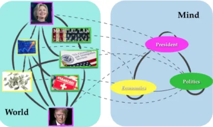
Figure 3.1:Concept Network
The world consists of a whole lot of objects with different kinds of features, which are the tangible representation of objects. There are physical world of living things, such as humans and animals. Human may have the features of age, height and nationality. There are intangibly world of knowledge, such as images and languages. The features for images may be the pixels and the features for language can be the words. When we see through the world, we perceive not a mass of features, but objects to which we automatically assign category labels. The categories refer to the sets of objects with similar features. Our perceptual system automatically segments the world into concepts. The concepts are the mental representation of categories. Therefore, when we try to perceive things, we extract from the features of physical representations and translate them into the concepts of mental representations.
While the concepts are the basics of our knowledge, relations between concepts are linking the concepts into the knowledge structures. It has long been recognized that concepts and relations are the foundations of
Figure 3.2:Concept & Relation Network
our knowledge and thoughts. Our lives and work depend on our understanding of knowledge of concepts and the web of relations.
The concepts and relation structure also presents in language and text. Concepts cannot be defined on their own but only in relation to other concepts, and the semantic relation can reflect the logical structure in the fundamental nature of thought Caplan & Herrmann (1993). Bean & Myaeng Green et al. (2013) noted that semantic relations play a critical role in how we represent knowledge psychologically, linguistically and computationally, and the knowledge representation relies heavily on the examination of internal structure, or in other words, internal relationships between semantic concepts.
Concepts and relations are often expressed in language and text. The words are the features of the language object, while the topics are the human interpretation of the concepts. The generation of language is to present the topic and relation structure in people’s mind through the words, and the understanding of language is to restore the structure from the words. Therefore, the understanding of language is a process of translating from the observable words to the topic and relation structure.
Traditional topic modeling focuses on the study of individual terms instead of relations between them. We shift the focus from terms to relations by focusing on the study of word pairs instead of individual words. KhooKhoo & Na (2006) states ‘frequently occurring syntagmatic relation between a pair of words can be part of our linguistic knowledge and considered lexical-semantic relations’. As Firth (1957) also puts it, ‘you shall
know a word by the company it keeps.’.
Therefore, in this thesis, we examine the pairwise relation through the pairwise relation graph. We formally define the pairwise relation graph as follows.
3.1
Pairwise Relation Graph
In this section, we formally define the pairwise relation graph as:
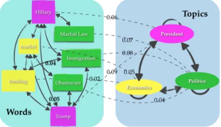
AssumeAis a set ofnwords{a1, a2, ..., an}, andCis a set ofm(m < n)topics{c1, c2, ..., cm}. The
pairwise relation graph consists of two important components.
a. Nodes. The graph has two types of nodes: words and topics. Each topic is a distribution over words. b. Node pairs. The graph has two types of node pairs: pairs of words or pairs of topics, with each pair representing the relation between each node pair. Each pair of topic is a distribution over word pairs.
Figure 3.3:word/topic network
3.2
Problem Formulation
Assume we have a corpus ofndocuments: {d1, d2, ...dn}, with vocabulary setV. We aim to extract the
pairwise relation graph from the collection of documents.
In the following two chapters, pairwise topic modeling is proposed to find the pairwise relation graph. Chapter 4 uses pairwise topic model to model the relation between the word pairs with relations extracted through information extraction tool, while Chapter 5 models the word pairs with the mutual information exceeding a threshold.
Actually, the pairwise topic model can also be extended to other fileds, a extension and modification of the pairwise topic model for image annotation can be found in Appendix.
Chapter 4: Pairwise Topic Model I
In this chapter, we will model the word pairs with relation extracted using information extraction tool. The pairwise relation graph can be obtained and the perplexity shows the pairwise topic model is more expressive than traditional topic models.
4.1
Introduction
Topic modeling is a good way to model language. Two important issues for the topic modeling are to select the text unit to carry one topic and how to model the relationship between the text units and their corresponding topics. For the first issue, different granularities are explored from word, phrase to sentence level. For the second issue, some works assume the semantic dependency between the sequential text units and try to model the dependency between the text unit sequence and their corresponding underlying topics using HMM (Gruber et al., 2007). Others use the syntactic structure information and then model the dependency among the hierarchical syntactic structure accordingly. Obviously, the model of the relationship is effective only when the choice of the text units ensures topical significance and there are explicit topical dependencies between the text units. However, few work view this two related issues as a whole and thus fail to model the relationship between two topics effectively. Therefore, the main problems for the models trying to find the underlying topic structure are twofolds. First, the text units selected may not have topical significance. Second, there is no definite relationship between the text units. In our work, we address the aforementioned two issues by firstly repre‘senting the document as the structured data and then modeling the explicit dependency embedded in this specific data structure. Thus, two problems need to be addressed here. The first is what kind of data structure to use. The second is how to model the data structure. For the first part, we will explore the entity pairs within relations as the data structure. The relation is a tuple ‘entity1, entity2, relation’. The data structure we explore here is ‘entity1, entity2’. Therefore, documents can be represented as a series of entity pairs. Only entities are used here, for they are more likely to convey central ideas and thus have a higher chance of carrying one topic. For example, in the sentence ‘As a democrat, Obama does support some type of universal health care’,
the relation is support ‘Obama, health care’. The central idea of this sentence is delivered actually by the two entities within it. Thus, the document is viewed as the representation of the closely related key idea pairs. Both the open relation and relation of a specific type are explored here. The relation of a specific type is better structured but can only represent the document from a certain perspective, while the open relation extraction are more flexible to capture more diverse relations, but may not as structured. Thus, the document represented by open relations could capture all aspects of key ideas of a document, while the relation of a specific type may only capture one aspect of all the key ideas.
As for the modeling of the structure, the explicit extraction of the targeted data structure, in this scenario, the entity pair, could to large extent, simplifies the modeling of the relation, since the relation is structured and much easier to model. Using the aforementioned example here, it is much easier to model the relation between ‘Obama’ and ‘health care’ than to model all the words ‘Obama does support some type of universal health care’. Also, the modeling of the relationship between entity pairs makes more sense compared to model the words in the whole sentence, since the entity pair will carry more topical dependency than simply two words appearing together. Here we only focus on the relation between the entities, ignoring the relationship between different relation pairs. This is actually a balance between simplicity and effectiveness. Six models are proposed here. They examine two aspects of the relationship within the entity pair. The first aspect examines whether to treat each entity or each entity pair as a unit. Further, if we treat each entity pair as a unit, whether it is generated from one topic or two. The second aspect examines how the dependency within one relation pair should be modeled. Both the dependency between the entity pair and the dependency between their underlying topics are modeled. As we can see, the modeling of the data structure is dependent on the selection of the structure, and the two are quite correlated.
4.2
Related Work
In this part, we would examine how the structure of the document is modeled in previous work. There are mainly three lines of work. In modeling the structure of a document, the first branch is to model the transition of the text units or their underlying topics. Two kinds of transition are modeled. The first is the transition of the observed text units. The second is the transition of the underlying topics of each text unit. The most
as the topical unit and models the relationship between words. He introduces a binary variable to control whether a consecutive word is dependent on the current topic and previous word, or dependent on the current topic only. Another way is to model the transition of the topic. Hongning Wang treats each sentence as a unit to carry one topic and views the generation of the consecutive underlying topics as a Hidden Markov Chain. Thus, the topic of one sentence depends on the topic of its previous sentence. Gruber Gruber et al. (2007) views each word as the unit to carry one topic and models their dependency of the topics underlying the words by introducing one binary variable to control whether a consecutive word has the same topic as the previous word or is to generate from the document topic distribution as in the LDA model. Another related work is done by Harr Chen et al. (2009). She also views each word as the topic carrier, and introduced a new topic ordering variable into LDA to permute the topic assignment of each word. Thus, the topic assignment for each word in LDA is not only dependent on the document-topic distribution, but also on this topic ordering variable. However, all of these methods have the inherited problem that the text unit to carry one topic may not have topical significance and these topic carriers have no significance in semantic dependency among each other. Therefore, the structure of the document data is not well-defined for the model to perform on, and thus the further modeling of the structure is not appropriate. Another branch to model the document structure is to use the syntactic knowledge. The most relevant model to ours is the syntactic topic model Boyd-Graber & Blei (2009). It is quite similar to our notion of modeling the data structure. In syntactic topic model, Boyd-Graber tried to model the syntactic tree structure resided in the Penne Tree Dataset by adding the dependency between the parent and child of the tree structure. To some extent, this work could be seen as the topic modeling of the structured data, since the document is represented by a series of syntactic trees and the tree structured is modeled by adding the dependencies between the parent and child of the syntactic tree. However, the author fails to fully examine the potential dependencies within one tree structure. Also, this work has two drawbacks from the perspective of modeling of the topical structure. The first is that the syntactic structure may not guarantee the semantic significance, since some of the words of a specific syntactic feature may not carry topical significance. Second, since the syntactic relationship may not have corresponding topical dependency, the topical transition assumption made when modeling the structure may not holds for most of time. Further, from the application perspective, the extraction of the syntactic tree is quite complex and the full exploration
of the tree structure is hard. Further, there are lots of works done on the combination of the LDA model and relation extraction. Yao modeled the relation tuples. In his work, one tuple is represented by a collection of features including the entities themselves. Thus, all these features are generated either by relation type or entity type, which are modeled separately. Although this line of study also focuses on the modeling of the relation, the main purpose of them is to do the relation extraction instead of modeling the document structure, thus may fall short of explicitly modeling entity pair structure.
4.3
Document Representation
In this section, we will examine why we choose the entity pairs as the data and how this structure could benefit the document representation and appropriate for topic modeling. We need to know how the topic modeling works before we select the data structure to use. The topic modeling actually takes advantage of the co-occurrence pattern of the text units to find the underlying topics. Intuitively, if two text units co-occur more within one document, they would have a higher chance to be in one topic. Thus, the redundancy of the co-occurred text units across the documents plays an important role to obtain good result. Further, for the structured data of the document, we not only need to model the underlying topics of the text units within the specific structure, but also to model that specific structure of the text units. Thus, we need to take advantage of the redundancy of the co-occurred text units with specific data structure to find the underlying topics.
Therefore, the two standards for us to select the data structure are: 1) the text unit should carry semantic and contextual topical significance and
2) the structure embedded within the text unit should have significance in dependency relation and at the same time simply enough to be captured. The selection of the entities as the text unit satisfies both of the standards.
4.4
Pairwise Topic Model
After we select the data structure to represent the document, we need to examine how to model the data structure. To model the entity pair structure, we need to explore the following two questions. The first is whether to treat each entity or each entity pair as a unit. And if each entity pair is treated as a unit, the further question should be whether it comes from one topic or two. The second is to examine how to model the dependency between two entities (if each entity is treated individually) and between the underlying topics
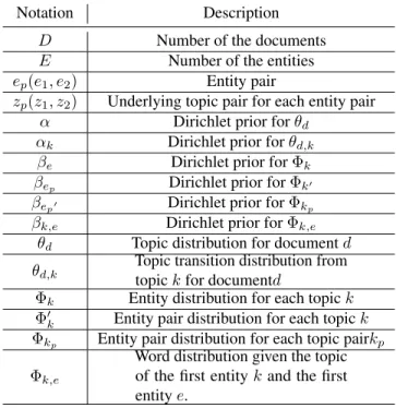
of two entities within an entity pair. Six models are proposed to answer the above two questions. The first three models all view each entity pair as one topic. The first model assumes each entity pair is generated from one topic. The second model assumes that each entity pair comes from two independent topics. The third model also views each entity pair is generated from two topics but the topics have dependency between each other. For the other three models, they all treat each entity as one topic. The fourth model assumes that the two entities are independent, but they come from two dependent underlying topics. The fifth model assumes that the two entities are dependent, but they come from two independent underlying topics. The sixth model assumes that both the entities pairs and topic pairs are dependent. Formally, we assume a corpus consists of D documents and the entity vocabulary size is E. There are K topics embedded in the corpus. For a specific document d, there are N entity pairs. Each model will be described in detail from three perspectives. The generative process of the model (the intuition behind the generative process), the graphical model for the generative process, and the joint probability for the model are introduced step by step in this section. Table 1 lists all the notations used in our models.
Table 4.1:Annotations in the generative process for relational topic model
Notation Description
D Number of the documents
E Number of the entities
ep(e1, e2) Entity pair
zp(z1, z2) Underlying topic pair for each entity pair
α Dirichlet prior forθd
αk Dirichlet prior forθd,k
βe Dirichlet prior forΦk
βep Dirichlet prior forΦk0
βep0 Dirichlet prior forΦkp
βk,e Dirichlet prior forΦk,e
θd Topic distribution for documentd
θd,k
Topic transition distribution from topickfor documentd
Φk Entity distribution for each topick
Φ0k Entity pair distribution for each topick
Φkp Entity pair distribution for each topic pairkp
Φk,e
Word distribution given the topic of the first entitykand the first entitye.
4.5
Model Description
After we select the data structure to represent the document, we need to examine how to model the data structure. To model the entity pair structure, we need to explore the following two questions. The first is whether to treat each entity or each entity pair as a unit. And if each entity pair is treated as a unit, the further question should be whether it comes from one topic or two. The second is to examine how to model the dependency between two entities (if each entity is treated individually) and between the underlying topics of two entities within an entity pair. Six models are proposed to answer the above two questions. The first three models all view each entity pair as one topic. The first model assumes each entity pair is generated from one topic. The second model assumes that each entity pair comes from two independent topics. The third model also views each entity pair is generated from two topics but the topics have dependency between each other. For the other three models, they all treat each entity as one topic. The fourth model assumes that the two entities are independent, but they come from two dependent underlying topics. The fifth model assumes that the two entities are dependent, but they come from two independent underlying topics. The sixth model assumes that both the entities pairs and topic pairs are dependent. Formally, we assume a corpus consists of D documents and the entity vocabulary size is E. There are K topics embedded in the corpus. For a specific document d, there are N entity pairs. Each model will be described in detail from three perspectives. The generative process of the model (the intuition behind the generative process), the graphical model for the generative process, and the joint probability for the model are introduced step by step in this section.
4.5.1
PTM-1
In PTM-1, each word pair is treated as one unit to be generated from one topic. The generative process is as follow.
1. Draw a topic - entity pair distribution for each topick(k1, k2= 1,2,3...K): Φk∼Dirichlet(βe)
2. For each document d (d = 1, 2,. . . D)
(a) Draw a document specific topic distribution:θd ∼Dirichlet(αk)
zp∼Dirichlet(βk)
Draw the entity pair from the topic-entity pair distribution ep∼Dirichlet(βk)
The joint probability of PTM-1 is as follows.
p(E, Z, θd, θd,k,Φz0|αk, βe p) = D Y d=1 Γ(PK k=1α) QK k=1Γ(α) K Y k=1 θd,kα−1 K Y k=1 (PE e=1)βe) QE e=1(βe) Φ0kβep−1 D Y d=1 K Y k=1 θnk d,k K Y k=1 Φ0knk,ep = (Γ( PK k=1αk) QK k=1Γ(αk) )D D Y d=1 K Y k=1 Θnk+αk−1 d,k ( ΓPE e=1βe QE e=1Γ(βe) )K K Y k=1 Φ0knk,ep+βep−1 (4.1)
4.5.2
PTM-2
In PTM-2, each word pair is treated as one unit to be generated from two topics. The generative process is as follow.
1. For each topic pair (k1, k2) (k = 1, 2, 3. . . K),
Draw a topic pair-entity pair distribution for each topic pair
Φkp∼Dirichlet(βkp)
2. For each document d (d = 1, 2,. . . D), a. Draw a document specific topic distribution θd∼Dirichlet(αk)
b. For each relation pair, draw the first and second topics from the document-topic distribution z1∼Categorical(θd)
z2∼Categorical(θd)
Draw the entity pair from the topic-entity distribution
e1∼Categorical(βk)
The joint probability of PTM-2 is as follows. p(E, Z, θd,Φkp|α, β 0 ep) = D Y d=1 Γ(PK k=1α) QK k=1Γ(α) K Y k=1 θd,kα−1 K Y k1=1 K Y k2=1 (PEp ep=1)β 0 ep) QEp ep=1(β 0 ep−1) Φβ 0 kp−1 kp D Y d=1 K Y k1=k2=1 θnk1+nk2 d K Y k1=1 K Y k2=1 Φnkkp,ep p =(Γ( PK k=1α) QK k=1Γ(α) )D D Y d=1 K Y k1=k2=1 Θnk1+nk2+α−1 d ( ΓPEp ep=1βep QEp ep=1Γ(βep) )K K Y k1=1 K Y k2=1 Φnkp,ep+β 0 ep−1 kp (4.2)
4.5.3
PTM-3
This model is the similar to R2 but it assumes that there is dependency between the two underlying topics. Thus, the whole generative process is as follow:
1. For each topic k (k = 1, 2, 3. . . K),
Draw a topic-entity pair distribution for each topic
Φp∼Dirichlet(βe)
2. For each document d (d = 1, 2,. . . D),
a. Draw a document specific topic distribution
θd∼Dirichlet(αk)
b. Draw a document specific topic transition distribution for each topic k (k =1,2,. . .,K).
θk0|k ∼Dirichlet(αk0|k)
For each entity pair. Draw the first topic from the document-topic distribution z1∼Categorical(θd)
Draw the second topic from the topic transition probability conditioned on the first topic. z2∼Categorical(θd,k0|k)
Draw the entity pair from the topic-entity pair distribution ep∼Categorical(Φk)
The joint probability for PTM-3 is as follow. p(E, Z, θd, θd,k,Φkp|α, αk, β 0 ep) = D Y d=1 Γ(PK z=1α) QK k=1Γ(α) K Y k=1 θαd−1 D Y d=1 Γ(PK k=1αk) QK k=1Γ(αk) K Y k=1 θα 0 k−1 d,k K Y k1=1 K Y k2=1 (PEp ep=1)βep) QE ep=1(βep−1) Φβ 0 ep−1 kp D Y d=1 K Y k=1 θnk1 d,k D Y d=1 K Y k2=1 θnk1,k2 d,k Kp Y kp=1 Φnkpkp,ep =(Γ( PK k=1α) QK k=1Γ(α) )D D Y d=1 K Y k2=1 Θnk1+α−1 d,k ( Γ(PK k=1αk) QK k=1Γ(αk) )D D Y d=1 K Y k2=1 Θnk1,k2+αk−1 d,k ( Γ PEp ep=1βep QEp ep=1Γ(βep) )K K Y k=1 Ep Y ep=1 Φnkp,ep+β 0 ep−1 kp (4.3)
4.5.4
PTM-4
From this model on, we will view each entity as one unit. Thus, model four will assume that two entities are generated from two dependent topics. The generative process of the first model is as follows:
1. For each topic k (k = 1, 2, 3. . . K), draw a topic-entity distribution for each topic
Φk ∼Dirichlet(βe).
2. For each document d (d = 1, 2, ... D), a. Draw a document specific topic distribution
θd∼Dirichlet(αk)
b. Draw a document specific topic transition distribution for each topic k. θk0|k ∼Dirichlet(αkprime|k)
c. For each relation pair,
Draw the topic of the first entity from the document-topic distribution z1∼Categorical(θk)
Draw the first entity from the topic-entity distribution
e1∼Categorical(Φk)
Draw the topic of the second entity from the topic transition probability conditioned on the first topic. z1∼Categorical(θk)
Draw the second entity from the topic-entity distribution
The joint probability for PTM-4 is as follows. p(E, Z, θd, θd,k,Φk|α, αk, βe) = D Y d=1 Γ(PK z=1α) QK k=1Γ(α) K Y k=1 θαd−1 D Y d=1 Γ(PK z=1αk) QK k=1Γ(αk) K Y k=1 θαk−1 d,k K Y k1=1 K Y k2=1 (PE e=1)βe) QE e=1(βe−1) Φβe−1 k D Y d=1 K Y k=1 θnk1 d,k D Y d=1 K Y k2=1 θnd,k1,k2 d,k K Y k Φnk,e k =(Γ( PK k=1α) QK k=1Γ(α) )D D Y d=1 K Y k1=1 Θnk1+α−1 d,k ( Γ(PK k=1αk) QK k=1Γ(αk) )D D Y d=1 K Y k2=1 Θnk1,k2+αk−1 d,k (Γ PE e=1βe QE e=1Γ(βe) )K K Y k=1 E Y e=1 Φnk,e+βe−1 k (4.4)
4.5.5
PTM-5
Different from the fourth model, this model models the dependency between two entities. The formal steps for the second generative model are:
1. For each topic k (k = 1, 2, 3. . . K), draw a topic-word distribution
Φk∼Dirichlet(βe)
2. For each topic k (k = 1, 2, 3. . . K) and an entity e (e = 1, 2, 3,. . .,E), draw an entity distribution
Φk,e∼Dirichlet(βk,e)
3. For each document d (d = 1, 2,. . . D),
a. Draw a document specific topic distribution
θd∼Dirichlet(αk)
b. For each relation pair,
Draw the topic of the first entity from the document-topic distribution. z1∼Categorical(θk)
Draw the first entity from the topic-entity distribution.
e1∼Categorical(Φk)
Draw the topic of the second entity from the document-topic distribution. e1∼Categorical(βe)
distribu-tion. e2∼Categorical(βk,e)
The joint probability for the fifth model is:
p(E, Z, θd,Φk,Φke|α, βe, βke) = D Y d=1 Γ(PK k=1α) QK k=1Γ(α) K Y k=1 θαd,k−1 K Y k=1 (PE e=1)βe) QE e=1(βe−1) Φβe−1 k K Y k=1 E Y e=1 (PE e=1)βke) QE e=1(βke−1) Φβke−1 ke D Y d=1 K Y k1=k2=1 θnk1+nk2 d K Y k1=1 Φnk1,e1 k K Y k2=1 E Y e1=1 Φnk2,ep k,e =(Γ( PK k=1α) QK k=1Γ(α) )D D Y d=1 K Y k=k1=k2=1 Θnk1+nk2+α−1 d ( ΓPE e=1βe QE e=1Γ(βe) )K K Y k1=1 Φnk1,e1+βe−1 k (Γ PE e=1βke QE e=1Γ(βke) )KE K Y k2=1 E Y e2=1 Φnk2,ep+βke−1 ke (4.5)
4.5.6
PTM-6
The sixth model inserts both the dependency between the entities and dependency between the underlying topics. The generative process is as follow:
1. For each topic k (k = 1, 2, 3. . . K), draw a topic-word distribution for each topic
Φk ∼Dirichlet(βe).
2. For each topic k (k = 1, 2, 3, ..., K) and an entity e (e = 1, 2, 3,. . .,E)
Draw an entity distribution
Φk,e∼Dirichlet(βk,e)
3. For each document d (d = 1, 2,. . . D),
a. Draw a document specific topic distribution
θ∼Dirichlet(αk)
b. Draw a specific topic transition distribution from topic k. θk ∼Dirichlet(αk)
c. For each relation pair, draw the topic of the first entity from the document-topic distribution z1∼Categorical(θk)
e1∼Categorical(βk)
Draw the topic of the second entity from the topic transition probability conditioned on the first topic. z2∼Categorical(αk0|k)
Draw the second entity from (topic, entity)-entity distribution. e2∼Categorical(βk,e)
The joint probability of the sixth model is:
p(E, Z, θd, θd,k,Φk,Φke|α, αk, βe, βke) = D Y d=1 Γ(PK z=1α) QK k=1Γ(α) K Y k=1 θdα−1 D Y d=1 Γ(PK z=1αk) QK k=1Γ(αk) K Y k=1 θαk−1 d,k K Y k=1 (PE e=1)βe) QE e=1(βe−1) Φβe−1 k K Y k=1 E Y e=1 (PE e=1)βe) QE e=1(βe−1) Φβke−1 ke D Y d=1 K Y k1=1 θnk1 d D Y d=1 K Y k2=1 θnk1,k2 d K Y k1=1 Φnk1,e1 k K Y k2=1 E Y e1=1 Φnk2,ep k,e =(Γ( PK k=1α) QK k=1Γ(α) )D D Y d=1 K Y k=k1=1 Θnk1+α−1 d,k ( Γ(PK k=1αk) QK k=1Γ(αk) )D D Y d=1 K Y k=k2=1 Θnk1,k2+αk−1 d,k ( Γ PE e=1βe QE e=1Γ(βe) )K K Y k1=1 Φnk1,e1+βe−1 k ( ΓPE e=1βke QE e=1Γ(βke) )KE K Y k2=1 E Y e2=1 Φnk2,ep+βke−1 ke (4.6)
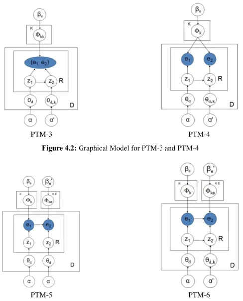
The graphical model of the generative process is shown in Figure 4.1-4.3.
PTM-1 PTM-2
PTM-3 PTM-4
Figure 4.2:Graphical Model for PTM-3 and PTM-4
PTM-5 PTM-6
Figure 4.3:Graphical Model for PTM-5 and PTM-6
4.6
Inference
We use the Gibbs Sampling to perform the parameter estimation and model inference. Because of the independency between the relations, two topics within one relation are sampled simultaneously. Table 4.2 lists all the notations used in Gibbs Sampling. Given the assignment of all the other hidden topic pairs, we use the following formula to sample the topic pairs for the model PTM-1 through model PTM-6.
Table 4.2:Annotations for the inference of relational topic model
Notation Description
n¬d,zi
i
Number of the entity pairs assigned to topicziin
docu-ment d except for the current entity pair n¬d,i(z
i1zi2)
Number of the second entity assigned to topicze2given
the topic of the first entity isze1except for the current
entity pair n¬zii,eip
Number of entity paireipassigned to topiczexcept for
the current entity pair. n¬zipi,eip
Number of entity paireip assigned to topic pair zp
except for the current entity pair n¬(zi
i1,ei1),ei2
Number of the second entityei2assigned tozi2, given
the first entity isei1 .
PTM-1: p(zi|E, Z¬i, α, βep) ∝ α+nd,zi PK k=1α+ PK k=1n −i d,k βep+n ¬i zi,eip PEp ep=1βep+ PEp ep=1n ¬i zi,ep (4.7) PTM-2 p(zi1, zi2|E, Z¬i, α, β 0 ep) ∝ α+n ¬i d,zi1=zi2 PK k=1α+ PK k=1n¬ i d,k βe0p+n ¬i zip,eip PEp ep=1β 0 ep+ PEp ep=1n ¬i zip,ep (4.8) PTM-3 p(zi1, zi2|E, Z¬i, α, αk, βe0p) ∝ α+n ¬i d,zi1 PK k=1α+ PK k=1n ¬i d,k αk+n¬d,i(zi 1,zi2) PK k=1αk+ PK k=1n ¬i d,(zi1,k) βe0p+n¬i zip,eip PEp ep=1β 0 ep+ PEp ep=1n ¬i zip,ep (4.9) PTM-4 p(zi1, zi2|E, Z¬i, α, β, βe0p) ∝ α+n ¬i d,zi1 PK k=1α+ PK k=1n¬ i d,k αk+n¬d,i(zi 1,zi2) PK k=1αk+P K k=1n¬ i d,(zi1,k) βe+n¬(zii 1,ei1)=(zi2,ei2) PE e=1βe+P E e=1(n¬zii1=zi2,e) (4.10)
PTM-5 p(zi1, zi2|E, Z¬i, α, β, βe0p) ∝ α+n ¬i d,zi1=zi2 PK k=1α+ PK k=1n¬ i d,k βe+nzi1,ei1 PE e=1βe+P E e=1(nzi1,ei1) βke+nzi2,ei1 PE e=1βke+P E e=1(nzi2,e) (4.11) PTM-6 p(zi1, zi2|E, Z¬i, α, β, βe0p) ∝ α+n ¬i d,zi1 PK k=1α+ PK k=1n¬d,ki αk+n¬d,i(zi1,zi2) PK k=1αk+P K k=1n¬d,i(zi1,k) βe+nzi1,ei1 PE e=1βe+P E e=1(nzi1,e) βke+nzi2,ei1 PE e=1βke+P E e=1(nzi2,e) (4.12)
4.6.1
Experiment
Data SetsFour data sets are used in the experiment. They are AP news articles, DUC 2004 task2, Medical Records and Elsevier article papers. Data Preprocessing For both the dataset AP news articles and DUC 2004 task 2 data, we run the open relation extraction tool Reverb to first extract all the open relations from the raw data and use the entity pairs only. For the medical records and Elsevier papers data, we use the entity recognition tool: Metamap (UMLS) to first extract both the symptoms and medications. Then we define the entity pair as the ‘symptom, medication’, in which the symptom and medication co-occurred in one section of one medical record as the one entity pair. We use the same strategy for the Elsevier data. We defined the entity pair as ‘gene, brain part’ and extract from the raw data the entities of both the genes and brain parts. The entities are only extracted from the articles except abstract, which is used for later evaluation. We then treat the gene and brain parts co-occurred in one sentence as entity pairs. The overall statistics of our dataset are listed in table 4.3.
Table 4.3:Dataset Statistics
Datasets # Files # Words before preprocessing # Words after Preprocessing
AP News 2250 76848 20153
DUC 2004 500 24713 6231
Medical Records 1249 67950 1148
Elsevier Papers 2058 141188 1132
and PTM-6, the data sparsity problem becomes obvious, as the number of parameters to be calculated becomes much larger. Therefore, we set all the hyper-parameters to be 0.01 to contradict the effect of the priors.
4.7
Result and Evaluation
4.7.1
Empirical Result
One advantage of the model is that it can capture the pairwise dependency between the topics. Next we will show a subset of the topics and how they are related. The result is obtained from the DUC 2004 dataset. The whole data set covers 50 news event and we only select the news covering 10 events. Therefore, the number of topic is set to 10. We sort the entities in each topic and the entity pairs in each pairwise topic according to their probabilities, and a subset of the topics and the top entity pairs relate them together are shown in Figure 4.4.
(a). Integrate PTM. (b). Separate PTM.
Figure 4.4:Topic Relatedness for DUC 2004 dataset
As we can see that the relatedness of the pairwise topics could be effectively explained.
4.7.2
Evaluation
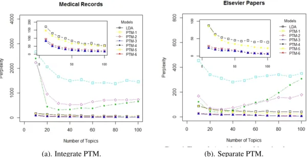
We use the perplexity to evaluate our modeling on the four datasets. The perplexity is widely used as the evaluation for the language model. It is the log likelihood on some unseen held-out, given a language model. For a corpus C of D documents, the perplexity is defined as: Where is the number of unit of text in document d, and w denotes one individual text unit. For traditional LDA, the text unit is word, and for the two models
proposed here, the text unit is entity. We compute and compare the perplexity of PTM-1 to PTM-6 with LDA on all the four datasets. For each dataset, we randomly held-out 80 percent of the document for training and 20 percent of the document for text. The perplexity on held-out data for all the six models is shown in Figure 4.5-4.6.
(a). Integrate PTM. (b). Separate PTM.
Figure 4.5:Perplexity comparison for AP news and DUC2004 Datasets
(a). Integrate PTM. (b). Separate PTM.
Figure 4.6:Perplexity comparison for Medical Records and Elsver Paper Datasets
Next we will try to answer the two questions asked at the beginning of section 5 according to the perplexity. First, we examine how the choice of one entity or entity pair as one unit could affect the model performance.
We compare the performance of the first three models and other models. LDA generally performs better than; while PTM-4, PTM-5 and PTM-6 perform better than LDA. Thus, the three models PTM-4, PTM-5 and PTM-6 perform better than PTM-1, PTM-2 and PTM-3 on all the four data sets, which is the same as our intuition that we should use one entity as a unit. To examine whether each entity pair carry one topic or two, we make comparison between PTM-1, PTM-2 and PTM-3. We find that the PTM-1 performs worst among all the models, meaning that the entity pair should be generated by two topics, which is also what intuition tells us. Further, comparing PTM-2 and PTM-3, we could find that PTM-3 performs relatively the same as PTM-2 on the dataset presented by the entity pairs of open relation, but better than PTM-2 on the entity pairs of a specific relation. The reason might be that the dependency relation between the entity pair of a specific type is much obvious than the dependency relation between the entity pairs of open relation. For example, the open relation might retrieve two entity pairs from the corpus, such as ‘Obama, healthcare’ and Healthcare, Obama’. They should be generated from the same topic pairs with opposite direction of dependency. Therefore, the two entity pairs will be assigned different topic pairs, for RTM only model one direction. This also explains why it works better on specific relation dataset, where the entity pairs have definite dependencies. Now we will try to find the best model to capture the dependency relationship for the entity pair structure. We have seen from the above discussion that if we treat entity pair as one unit, whether we should model the topic dependency depends largely on the kind of structure we model. That is, if there is obviously one direction dependency between the entities, the model of dependency between their underlying topics is preferred; while the modeling of dependency makes no difference to the entities that have no definite direction of dependency. Now we will examine how the modeling of dependency affects the performance when each entity is treated as one individual topic carrier. The pattern we get from PTM-4 to PTM-6 on the four different datasets are quiet consistent. PTM-6 performs better than PTM-5 and PTM-5 performs better than PTM-4 on all the four datasets. Therefore, PTM-6 is the best model to capture the entity pair structure.
Chapter 5: Pairwise Topic Model II
In this chapter, we generalize the word pairs to include all the pairs with mutual information exceeding a certain threshold.
5.1
Introduction
The spread of the WWW has led to the boom of explosive Web information. One of the core challenges is to understand the massive document collection with topic transition and evolution.
Among content analysis techniques, topic modeling represents a set of powerful toolkits to describe the process of documents generation. Generally, topic models are based on the unigram and the term based topic models are proved to be a good way to model the languages. While individual words and the hidden topics are the building blocks of language, relations between the terms and underlying topics act as cement that links the words into language structures. This chapter shifts the focus from the terms to the relations by modeling the word pairs instead of individual words. We explore the term association and show the shift to relation achieve greater effectiveness and refinement in topic modeling. To the best of our knowledge, this is the first effort to explicitly model the semantically dependent word pairs.
In this chapter, word pairs refer to two words that are semantically related. They cooccur in the same sentence as in original order, but not necessarily to be consecutive. One advantage of pairwise topic relation is its coverage of the long-range relationship. For example, in the sentence ‘Obama supports healthcare’, the extracted word pairs should be ‘obama, support’, ‘support,healthcare’ and ‘obama, healthcare’. Also, the modeling of relation can in turn facilitates the topic extraction. The relation between ‘obama’ and ‘healthcare’ makes it much easier to identify ‘obama’ as a ‘politician’, and ‘healthcare’ as a ‘policy’. In this work, we will first extract the semantic dependent word pairs through mutual information and then model the dependency within the word pairs.
By considering the semantic dependency between two words, we propose two ways to establish our topic modeling. The first way is to model the related words as a whole unit; the other way is to model each word as
separate units with dependency constraints. The dependencies between the word pairs (if the words are treated separately) and their underlying topics are modeled simultaneously. With dependencies incorporated, it is natural to discover topics hidden in the contexts and find out the evolution trajectories and transition matrix for all discovered topics.
Therefore, the novelties of this part of thesis are as follow.
•Documents are treated as structured data with relations, represented by a bag of word pairs, to facilitate the modeling of the document representation.
• Two different ways of topic modeling with semantic dependencies between words are proposed to characterize the word pair structure and then to capture the pairwise relationship embedded in the structured data.
• We have conducted a thorough experimental study on the news data and literature data to test the performance of topic discovery and then empirically evaluate the evolution and transition among the discovered topics.
This chapter is organized as follows. The second section covers the related work. In the third Section, we propose to examine the document representation, and in Section 4 we describe all the models in details. We will elaborate the model inference process for the proposed models in the fifth Section. Section 6 discusses how the PTM can help facilitate word/topic relation analysis. The experiment and evaluation will be included in Section 7 and Section 8 respectively; while in Section 9, we will draw the conclusion and discuss about future work.
5.2
Related Work
Over the years, topic evolution and transition have been studied intensively Chang & Blei (2009), Jo et al. (2011), Wang & McCallum (2006). Miscelleous methods are applied to detect more informative and distinctive topics. Most of the work explores the probabilistic topic modeling over text Blei et al. (2003), Griffiths & Steyvers (2004), Hofmann (2001) and further to integrates topic modeling over text with time series analysis Blei & Lafferty (2006), Wang & McCallum (2006) to obtain the topic evolution. But the pre-defined time granularity makes these time-sensitive models unreliable unless the time interval is appropriately chosen. He
only use citation information, the text information is ignored.
Therefore, in this chapter, we try to find a more expressive topic modeling to explore the topic transition and evolution. The main concern for traditional topic modeling Blei et al. (2003) is its ‘bag of words’ assumption. Researchers try different methods to overcome the restriction. One of the early efforts to model the relationship among the topics is the CTM model Blei & Lafferty (2007). Instead of drawing the topic proportions of a document from a Dirichlet distribution, CTM model uses a more flexible logistic normal distribution introduce the covariance among the topics. However, this model could only examine if the two topics are related without showing the direction and degree of relatedness. Rather than modeling the correlation implicitly from the topic generation process, most work models the relationship explicitly, either by modeling the relationship between the topics Gruber et al. (2007), Wang et al. (2011), or between the words Wang et al. (2007), Wallach (2006). These models assume the relation between the words or sentences in sequential order. However, the words in sequential order don’t necessarily relate to each other semantically, making the assumption unreasonable. Also, they can not model the words and topics simultaneously.
Except to model the sequential words, Chen et al. (2009) or the syntactic information Boyd-Graber & Blei (2009) also model the position and syntactic structure. Among all these methods, none explores the relation between word pairs.
Therefore, in our work, we will investigate the topic dependency among semantically dependent words. By firstly extracting the potential dependent word pairs, we are more confident to capture meaning dependency relationship and furthermore meaningful topic transition and evolution.
5.3
Document Representation
The pairwise topic model is to model the data composed of word pairs and links between them. It embeds the word pairs in a latent space that explains both the word and the topic relationship. We will give more insight into the document space of word pairs in this section.
Document Manipulation with Mutual Information. Different from the traditional topic modeling of manipulating the individual words, the pairwise topic model takes word pairs as input. The topic model with semantic relationship will be effective only when the processed word pairs do have significant topic dependencies between each other. Accordingly, we extract prominent word pairs out of the documents. We
measure the semantic dependency between two words through mutual information. The mutual information I(w1, w2)between two wordsw1andw2is defined as:
I(w1, w2) =p(w1, w2) log p(w1)p(w2) p(w1, w2) ∝ N w1 s Nsw2 N(w1,w2) s (5.1) WhereNw1
s andNsw1 are the number of times wordw1and wordw2appear respectively in one sentence,
whileN(w1,w2)
s are the timesw1andw2appear in the same sentence.
Therefore, we assume the two words have semantic dependency when their mutual information exceeds a pre-defined threshold. Hence, we change the representation of the unstructured documents into the structured data in form of word pairs, and then model the explicit dependency in word pairs.
By taking the semantic dependency, namely relationship, between two words, this model will offer us more insight for document analysis.
5.4
Pairwise Topic Model
The pairwise topic model(PTM) is a generative model of document collections. Different from previous work, it is to examine the dependency between the words and their underlying topics via the word pairs, assuming the dependency within the word pair and independency among the word pairs. Thus, the key part is to model the dependency between two words and theirs corresponding topics. We propose two models: PTM-1 and PTM-2 to examine the semantic dependency in detail.
The first model, the integrated pairwise topic model (PTM-1), arises from the intuition that two words and their link together represent a semantic unit. Two words with the link form one unit generated by the whole topic pair, with the second topic dependent on the first one.
The second model, the separated pairwise topic model (PTM-2), treats each word as one individual unit and explicitly model the relationship between words. In PTM-2, the generation of the second word is determined not only by its topic, but also by the first word and its corresponding topic. Both PTM-1 and PTM-2 allow each document to exhibit multiply topic transition with different proportions. We use the following terminology and notation in Table 5.1 to describe the data, latent variables and parameters in the PTM models.
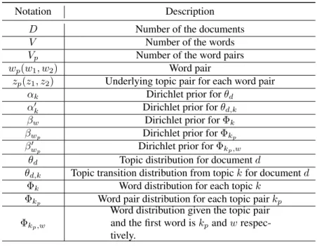
Table 5.1:Annotations in the generative process for topic evolution model.
Notation Description
D Number of the documents
V Number of the words
Vp Number of the word pairs
wp(w1, w2) Word pair
zp(z1, z2) Underlying topic pair for each word pair
αk Dirichlet prior forθd
α0k Dirichlet prior forθd,k
βw Dirichlet prior forΦk
βwp Dirichlet prior forΦkp
βw0p Dirichlet prior forΦkp,w
θd Topic distribution for documentd
θd,k Topic transition distribution from topickfor documentd
Φk Word distribution for each topick
Φkp Word pair distribution for each topic pairkp
Φkp,w
Word distribution given the topic pair and the first word iskpandw
respec-tively.
processes.
For PTM-1, the generative process is as follow:
1. For each topic pairkp(k1, k2)(k1,k2= 1, 2, 3,. . . K),
(a) Draw a (topic pair - word pair) distribution for each topic pairkp:
Φ(kp)∼Dirichlet(βwp)
2. For each document d (d∈1, 2,. . ., D), (a) Draw a document specific topic distribution:
θd∼Dirichlet(αk)
(b) Draw a document specific topic transition distribution for each topic k: θd,k∼Dirichlet(α0k)
(c) For each word pair
(i) Draw the first topic from the document-topic distribution: z1∼Categorical(θd)
z2∼Categorical(θd,z1)
(iii) Draw the word pair from the topic pair-word pair distribution: wp∼Categorical(Φzp)
During the generative process, the word pair is treated as one unit and generated from the dependent topic pair. This model is to check if two words as a text unit is sufficient to capture the topic transition.
Next, we propose PTM-2 to simulate the more intricate relationship between the words of a pair adding the dependency between the words. The generative process for PTM-2 is:
1. For each topic k (k = 1, 2, 3,. . ., K),
(a) Draw a topic-word distribution for each topic:
Φk ∼Dirichlet(βw)
2. For each topic pairkp(k1, k2)(k1, k2= 1, 2, 3,. . ., K) and a word w (w = 1, 2, 3,. . ., V)
(a) Draw a word distribution:
Φkp,w∼Dirichlet(β 0
w)
3. For each document d (d = 1, 2,. . ., D), (a) Draw a document specific topic distribution:
θd∼Dirichlet(αk)
(b) Draw a specific topic transition distribution from topic k: θd,k∼Dirichlet(α0k)
(c) For each word pair,
(i) Draw the topic of the first word from the document-topic distribution: z1∼Categorical(θk)
(ii) Draw the first word from the topic-word distribution: w1∼Categorical(Φz1)
(iii) Draw the topic of the second word from the topic transition distribution conditioned on the first topic: z2∼Categorical(θz1)
(iv) Draw the second word from (topic pair, word)∼word distribution: w2∼Categorical(Φ(zp,w1)))
PTM-2 treats every individual word in the pair as the text unit. In addition to the topic of the second word, the first word and its corresponding topic also contribute to the generation of the second word.
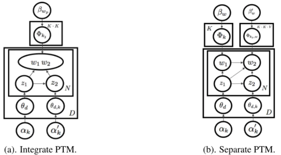
(a). Integrate PTM. (b). Separate PTM.
Figure 5.1:Two ways for graphical representation for pairwise topic modeling.
The joint probability of PTM-1 can be illustrated as following:
p(W, Z, θd, θd,k,Φzp|αk, α 0 k, βwp) = D Y d=1 Γ(PK z=1αk) QK k=1Γ(αk) K Y k=1 θαk−1 d,k D Y d=1 K Y k=1 Γ(PK k0=1α0k0) Qk k0=1Γ(α0k0) K Y k0=1 θαd,kk0 |k0 −1 K Y k1=1 K Y k2=1 Γ(PVp wp=1βwp) QVp wp=1Γ(βwp) QVp wp=1 Φβkwp−1 p D Y d=1 K Y k1=1 θnk1 d D Y d=1 K Y k1 K Y k2=1 θnd,k2|k1 d,k1 K Y k1=1 K Y k2=1 Vp Y wp=1 Φnkkp,wp p =(Γ( PK k=1αk) QK k=1Γ(αk) )D D Y d=1 D Y k=1 θαk+nk−1 d (Γ( PK k0=1αk0) QK k0=1Γ(αk0) )DK D Y d=1 K Y k=k1=1 K Y k0=k 2=1 θαk0 |k+nd,k2|k1−1 d,k (Γ( PVp wp=1βwp) QVp wp=1Γ(βwp) )KK K Y k1=1 K Y k2=1 Vp Y wp=1 Φβkwp+nkp,wp−1 p (5.2)
The joint probability of PTM-2 is: p(W, Z, θd, θd,k,Φk,Φ0kp|αk, α 0 k, βw, β0wp) = D Y d=1 Γ(PK k=1αk) QK k=1Γ(αk) K Y k=1 θαk−1 d,k D Y d=1 K Y k=1 Γ(PK k0=1α0k0) Qk k0=1Γ(α0k0) K Y k0=1 θαd,kk0 |k0 −1 K Y k=1 Γ(PV w=1βw) QV w=1Γ(βw) QV w=1 Φβw−1 k K Y k1=1 K Y k2=1 Γ(PV w0=1βw0 p) QV w0=1Γ(βw0p) QV w0=1 Φβ 0 wp−1 kp,w0 D Y d=1 K Y k1=1 θnk1 d D Y d=1 K Y k1=1 K Y k2=1 θnd,k2|k1 d,k1 K Y k1=1 V Y w1=1 Φnk1 k1 K Y k1=1 K Y k2=1 V Y w1=1 V Y w2=1 Φnkkp,wp p,w1 =(Γ( PK k=1αk) QK k=1Γ(αk) )D K Y d=1 D Y k=1 θαk+nk−1 d (Γ( PK k0=1αk0) QK k0=1Γ(αk0) )DK D Y d=1 K Y k=k1=1 K Y k0=k 2=1 θαk0 |k+nd,k2|k1−1 d,k (Γ( PV w=1βw) QV w=1Γ(βw) )K K Y k=1 V Y w=1 Φβw+nk,w−1 k (Γ( PV w=1βw0p) QV w=1Γ(βw0p) )KKV K Y k1=1 K Y k2=1 K Y w1=1 V Y w2=1 Φβ 0 wp+nkp,wp−1 k (5.3)
Overall, both the models can capture the topic dependency of a word pair and find the topic transition and be more expressive than traditional topic models.
The two generative processes are illustrated as probabilistic graphical models in Figure 5.1.
5.5
Inference
We use Gibbs sampling to perform model inference. Due to the space limit, we leave out the derivation details and only show the sampling formulas. The notations for the sampling formulas are as shown in Table 5.2.