UCLA
UCLA Electronic Theses and Dissertations
TitleScalable Methods for Big Time-To-Event Data
Permalink
https://escholarship.org/uc/item/3h95x3km
Author
Kawaguchi, Eric Shinya
Publication Date
2019
Peer reviewed|Thesis/dissertation
UNIVERSITY OF CALIFORNIA Los Angeles
Scalable Methods for Big Time-To-Event Data
A dissertation submitted in partial satisfaction of the requirements for the degree Doctor of Philosophy in Biostatistics
by
Eric Shinya Kawaguchi
c
Copyright by Eric Shinya Kawaguchi
ABSTRACT OF THE DISSERTATION
Scalable Methods for Big Time-To-Event Data
by
Eric Shinya Kawaguchi
Doctor of Philosophy in Biostatistics University of California, Los Angeles, 2019
Professor Gang Li, Chair
Computational advancements and cost efficiency over the recent years have made big data readily available to researchers. In the biomedical and public health fields analyzing time-to-event data, where the outcome of interest is a time-time-to-event endpoint, is of particular interest. However, big time-to-event data poses many challenges to currently-available sta-tistical methods due to the large number of covariates and/or observations one can observe. In this dissertation we propose scalable sparse regression methods for both big right-censored and competing risks time-to-event data. We extend the recently-introduced broken adaptive ridge (BAR) regression procedure to both the Cox (1972) proportional hazards for right-censored data and theFine and Gray(1999) proportional subdistribution hazards model for competing risks data, establish its large-sample properties under diverging dimension, and develop computational software that is scalable to big time-to-event data.
The dissertation of Eric Shinya Kawaguchi is approved. Xinshu Xiao
Hua Zhou Marc Adam Suchard Gang Li, Committee Chair
University of California, Los Angeles 2019
To God, for blessing me with this wonderful opportunity and for placing such incredible mentors, colleagues, and friends into my life. To my parents, Douglas and Mari, and sister,
Traci, for encouraging me to explore and pursue my interests and passions. To my wife, Lucia, for her comfort, support, and love throughout this endeavor.
TABLE OF CONTENTS
1 Introduction . . . 1
2 Preliminaries and literature review . . . 7
2.1 Modeling the hazard function for right-censored time-to-event data . . . 7
2.2 Penalized variable selection procedures for the Cox proportional hazards model 9 2.3 Modeling the subdistribution hazard function for competing risks data . . . 12
3 Broken adaptive ridge for the Cox proportional hazards model with appli-cations to sparse high-dimensional massive sample size (sHDMSS) data . . 16
3.1 Methodology . . . 17
3.1.1 Cox’s broken adaptive ridge regression and its large sample properties 17 3.1.2 Efficient implementation BAR for sparse high-dimensional massive sample size (sHDMSS) data . . . 21
3.2 Simulations . . . 23
3.2.1 BAR estimator for varying values of ξn . . . 24
3.2.2 Model selection and parameter estimation . . . 24
3.2.3 Sparse high-dimensional massive sample size data . . . 26
3.3 Pediatraic trauma mortality . . . 28
3.4 Discussion . . . 30
Appendix to Chapter 3 . . . 31
A3.1 Regularity conditions for Theorem 3.1 . . . 31
A3.2 Proof of Theorem 3.1 . . . 33
A3.4 The CLG algorithm for Cox ridge regression as explained in Section
3.1.2 . . . 55
A3.5 Additional simulation results for Section 3.2.1 . . . 57
A3.6 Additional simulation results for Section 3.2.2 . . . 60
4 Broken adaptive ridge for the Fine-Gray proportional subdistribution haz-ards model with applications to large-scale competing risks data . . . 62
4.1 Methodology . . . 63
4.1.1 Preliminaries: Competing risks data, model, and parameter estimation for fixed model dimension . . . 63
4.1.2 Broken adaptive ridge estimation for the proportional subdistribution hazards model under diverging model dimension . . . 65
4.1.3 A cyclic coordinate-wise BAR algorithm . . . 68
4.1.4 Scalable parameter estimation via forward-backward scan . . . 70
4.2 Simulation study . . . 72
4.2.1 Simulation setup . . . 72
4.2.2 Variable selection and parameter estimation performance . . . 73
4.2.3 Computational efficiencies . . . 75
4.3 End-stage renal disease . . . 76
4.4 Discussion . . . 78
Appendix to Chapter 4 . . . 79
A4.1 Regularity conditions . . . 79
A4.2 Proof of Lemmas for Theorem 4.1 . . . 82
A4.3 Proof of Theorem 4.1 . . . 96
A4.4 Proof of Theorem 4.2. . . 98
A4.6 Proof of Lemma 4.1 . . . 101
A4.7 BAR implementation via CCD . . . 102
A4.8 Additional figures and tables . . . 103
5 Fast and scalable Fine-Gray regression and cumulative incidence function estimation . . . 110
5.1 Data structure and model . . . 110
5.1.1 Parameter estimation for unpenalized Fine-Gray regression . . . 111
5.1.2 Estimating the cumulative incidence function . . . 112
5.1.3 Penalized Fine-Gray regression for variable selection . . . 113
5.2 Forward-backward scan for parameter estimation . . . 114
5.3 The fastcmprsk package . . . 116
5.3.1 Simulating competing risks data . . . 116
5.3.2 Unpenalized parameter estimation and inference . . . 117
5.3.3 Cumulative incidence function and interval/band estimation . . . 120
5.3.4 Penalized Fine-Gray regression via forward-backward scan . . . 122
5.4 Simulation studies . . . 123
5.4.1 Comparison to the crr package . . . 124
5.4.2 Comparison to the crrp package . . . 125
5.5 End-stage renal disease . . . 127
5.6 Discussion . . . 129
Appendix to Chapter 5 . . . 130
A5.1 Data generation scheme . . . 130
LIST OF FIGURES
3.1 Path plot for BAR regression with varying ξn and: (b) λn = log(pn), (c) λn = 0.5 log(pn), and (d) λn = 0.75 log(pn) with estimates averaged over 100 Monte Carlo simulations of size n = 300, pn = 100, and censoring rate ≈ 25%. Path plot for ridge regression (d) with varying ξn is also included as a comparison. . . 25 3.2 Path plots for mCox-LASSO and BAR regression: (a) Path plot for mCox-LASSO
regression, where the black dashed line represents the estimates when using cross validation to find the optimal value of the tuning parameter; (b) Path plot for BAR regression with ξn = 1 and varying λn, where the black solid and dashed line represent estimates for λn = ln(n) and λn = ln(dn), respectively; (c) Path plot for BAR regression with λn = ln(n) and varying ξn, where the black solid line represent the estimates for BAR when ξn = 1. . . 28 A3.1 Path plot for BAR regression with varying ξn and: (b) λn = log(pn), (c) λn =
0.5 log(pn), and (d) λn = 0.75 log(pn) with estimates averaged over 100 Monte Carlo simulations of size n = 300, pn = 40, censoring rate ≈ 25%, and β = (β∗,β∗,β∗,0pn−30) where β
∗ = (0.40,0,0.45,0,0.50,0.55,0,0,0.70,0.80). Path
plot for ridge regression (d) with varying ξn is also included as a comparison. . . 57 A3.2 Path plot for BAR regression with varying ξn and: (b) λn = log(pn), (c) λn =
0.5 log(pn), and (d) λn = 0.75 log(pn) with estimates averaged over 100 Monte Carlo simulations of size n = 300, pn = 40, censoring rate ≈ 60%, and β = (β∗,0pn−10) where β
∗ = (0.40,0,0.45,0,0.50,0.55,0,0,0.70,0.80). Path plot for
ridge regression (d) with varying ξn is also included as a comparison. . . 58 A3.3 Path plot for BAR regression with varying ξn and: (b) λn = log(pn), (c) λn =
0.5 log(pn), and (d) λn = 0.75 log(pn) with estimates averaged over 100 Monte Carlo simulations of size n = 1000, pn = 100, censoring rate ≈ 25%, and β = (β∗,β∗,β∗,0pn−30) where β
∗ = (0.40,0,0.45,0,0.50,0.55,0,0,0.70,0.80). Path
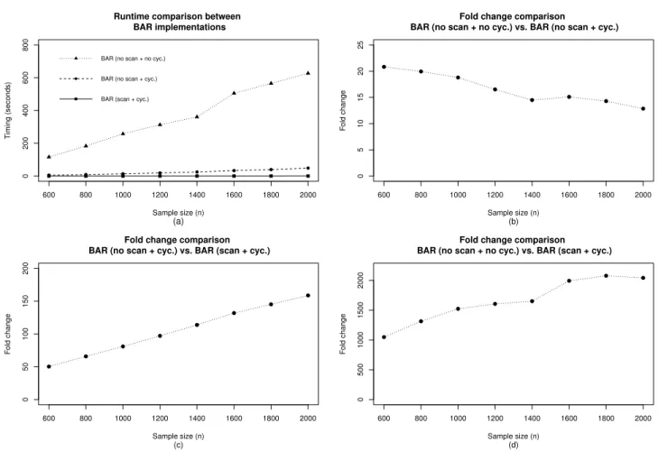
4.1 Runtime comparison between three BAR(λn) implementations (cyc. =cycBAR described in Section 4.1.3; scan = forward-backward scan described in Section 4.1.4). 75 A4.1 Graphs of β1 = g1(β2) (solid line) and β2 = g2(β1) (dotted line) under selected
scenarios, which by Theorem 2, intersect at the fixed-point of g(β1, β2). . . 103
A4.2 An illustration of thecycBARalgorithm in a zoomed in picture of Figure S1(a). The BAR estimator is the fixed point of g(β1, β2), which, by Theorem 2, is the
intersection of β1 =g1(β2) andβ2 =g2(β1). . . 104
A4.3 Path plot for BAR regression with varyingξn and several fixed values ofλnwhere
n = 300 and pn= 40. The path plots are averaged over 100 simulations. . . 105 A4.4 Path plot for BAR regression with varyingξn and several fixed values ofλnwhere
n = 300 and pn= 100. The path plots are averaged over 100 simulations. . . 106 A4.5 Path plot for BAR regression with varyingξn and several fixed values ofλnwhere
n = 700 and pn= 40. The path plots are averaged over 100 simulations. . . 107
5.1 CIF estimate and corresponding 95% confidence intervals between tL = 0.2 and
tU = 0.9. . . 122 5.2 Path plot for LASSO-penalized Fine-Gray regression in our toy example. . . 124 5.3 Runtime comparison between fastCrr and crr with and without variance estimation.125 5.4 Runtime comparison between thecrrpandfastcmprskimplementations of LASSO,
SCAD, and MCP penalization. Solid and dashed lines represent the crrp and
fastcmprsk implementation, respectively. Square, circle, and triangle symbols denote the penalties MCP, SCAD, and LASSO, respectively. . . 126 5.5 Point estimate and 95% confidence intervals reported by fastCrr (using 100
LIST OF TABLES
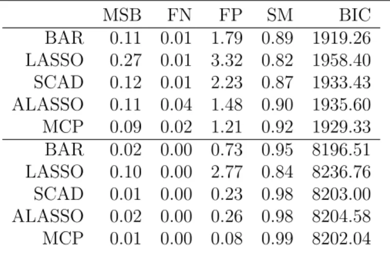
3.1 (Moderate dimension and sample size) Simulated estimation and variable selec-tion performance of BAR, LASSO, SCAD, ALASSO, and MCP where the BIC criterion was used to select the tuning parameters via a grid search. (MSB = mean squared bias; FN = mean number of false positives; FP = mean number of false negatives; SM = similarity measure; BIC = average BIC score; Each entry is based on 100 Monte Carlo samples of size n = 300 (top), and 1000 (bottom),
pn = 100, censoring rate ≈25%.) . . . 26 3.2 (Sparse high dimensional and massive sample size) Estimation and variable
se-lection results for BAR and massive Cox regression with LASSO penalty (mCox-LASSO, Mittal et al.(2014)) for a simulated sHDMSS dataset with n= 200,000,
pn = 20,000, and qn = 60. (Bias = ||βˆ−β0||2; FP= number of false positives;
FN = number of false negatives.) . . . 27 3.3 (Pediatric NTDB data) Comparison of mCox-LASSO and BAR regression for the
pediatric NTDB data. (mCox-LASSO (CV) and mCox-LASSO (BIC) correspond to mCox-LASSO using cross validation and BIC selection criterion, respectively. BAR (BIC) denotes BAR using the BIC selection criterion while fixing ξn = log(pn). The training set has a sample size of 168,000 while the test set used for the c-index has a sample size of 45,555.) . . . 29 A3.1 Simulated estimation and variable selection performance of BAR, LASSO, SCAD,
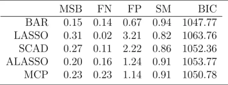
ALASSO, and MCP where the BIC criterion was used to select the tuning pa-rameters via a grid search. (MSB = mean squared bias; FN = mean number of false positives; FP = mean number of false negatives; SM = similarity measure; BIC = average BIC score; Each entry is based on 100 Monte Carlo samples of size n = 300,pn = 40, censoring rate≈25% , andβ = (β∗,β∗,β∗,0pn−30) where
A3.2 Simulated estimation and variable selection performance of BAR, LASSO, SCAD, ALASSO, and MCP where the BIC criterion was used to select the tuning pa-rameters via a grid search. (MSB = mean squared bias; FN = mean number of false positives; FP = mean number of false negatives; SM = similarity mea-sure; BIC = average BIC score; Each entry is based on 100 Monte Carlo samples of size n = 300, pn = 40, censoring rate ≈ 60%, and β = (β∗,0pn−10) where
β∗ = (0.40,0,0.45,0,0.50,0.55,0,0,0.70,0.80)) . . . 60 A3.3 Simulated estimation and variable selection performance of BAR, LASSO, SCAD,
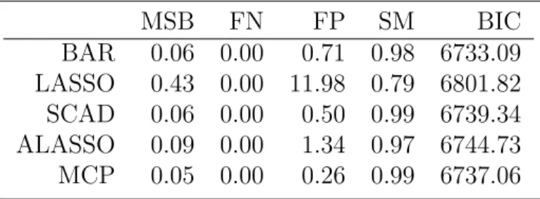
ALASSO, and MCP where the BIC criterion was used to select the tuning pa-rameters via a grid search. (MSB = mean squared bias; FN = mean number of false positives; FP = mean number of false negatives; SM = similarity measure; BIC = average BIC score; Each entry is based on 100 Monte Carlo samples of size n = 1000, pn = 100, censoring rate ≈ 25% , and β = (β∗,β∗,β∗,0pn−30)
where β∗ = (0.40,0,0.45,0,0.50,0.55,0,0,0.70,0.80)) . . . 61 4.1 Estimation and selection performance of BAR along with LASSO, ALASSO,
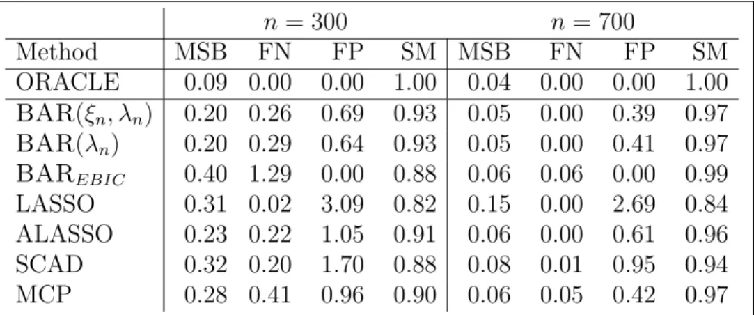
SCAD, and MCP. (BAR(ξn, λn): ξnandλnare found using a two-dimensional grid search; BAR(λn): ξn = log(pn) and λn is found through a grid search; BAREBIC:
ξn = log(pn) and λn= log(pn); MSB = mean squared bias; FN = mean number of false positives; FP = mean number of false negatives; SM = average similarity measure; Censoring rate ≈ 30%; pn = 40;qn = 6. The BIC criterion is used for tuning parameter selection for all methods except for BAREBIC. Each entry is based on 100 Monte Carlo samples. ) . . . 74 4.2 Analysis results of a USRDS data using BAR with four different implementations
along with MCP and SCAD (BAR(λn): ξn = log(pn) and λn selected through a grid search; BAREBIC: ξn = λn = log(pn); cyc. = cycBAR; lin. = forward-backward scan; Except for BAREBIC, BIC was used to select tuning parameters; *The original BAR(λn) without cycBAR and forward-backward scan did not finish after 96 hours.) . . . 78
A4.1 Additional simulation results for model comparison. Based on 100 replications withρ= 0.5,β1 = (β∗,0pn−10) whereβ
∗ = (0.40,0.45,0,0.50,0,0.60,0.75,0,0,0.80),
censoring rate ≈33% and type 1 event rate≈41%. . . 108 A4.2 Additional simulation results for model comparison. Based on 100 replications
withρ= 0.5,β1 = (β∗,0pn−10) whereβ
∗ = (0.40,0.45,0,0.50,0,0.60,0.75,0,0,0.80),
censoring rate ≈33% and type 1 event rate ≈32%(π= 0.4) and ≈43%(π= 0.75).108 A4.3 Additional simulation results for model comparison. Based on 100 replications
withρ= 0.5,β1 = (β∗,β∗,β∗,0pn−30) whereβ
∗ = (0.40,0.45,0,0.50,0,0.60,0.75,0,0,0.80),
censoring rate ≈33% and type 1 event rate≈41%. . . 109 A4.4 Additional information about the USRDS subset. Summary of event count (%)
observed for the training (n = 125,000) and test (n = 100,000) sets for the USRDS subset. (Disc: Discontinued dialysis; Recov: Renal function recovery; RC: Right censored including loss-to-follow up and end of study time.) . . . 109
5.1 Currently available functions in fastcmprsk (as of May 15, 2019). . . 116 5.2 Coverage probability (and standard errors) of 95% confidence intervals for β11 =
0.4. Standard errors for fastCrr are obtained using 100 bootstrap samples. . . . 125 5.3 Timing comparison using a subset of the USRDS dataset. The first two rows
correspond to unpenalized Fine-Gray regression with and without variance es-timation using crr and fastCrr. The last three rows correspond to penalized Fine-Gray regression using crrp and fastCrrp. . . 128
ACKNOWLEDGMENTS
I would like to express my sincere gratitude to my dissertation advisor, Dr. Gang Li, for his guidance, advice, support, encouragement, and most importantly, patience, during my academic career at UCLA. I have learned tremendously under his direction. Many thanks are also due to my committee members: Drs. Marc A. Suchard, Hua Zhou, and Xinshu Xiao for their valuable comments, insights, and suggestions. I greatly enjoyed getting to know them during this process. I would like to extend my thanks to Drs. Randall Burd and Sushil Mittal for access to the National Trauma Data Bank dataset used in Chapter 3 and to Dr. Jenny I. Shen for access to the United States Renal Data Systems dataset used in Chapters 4 and 5. Lastly, I am also very thankful for my fellow cohort members and colleagues, I could not imagine starting and finishing this journey without you all.
VITA
2009–2013 B.S. (Mathematics), California State Polytechnic University, Pomona, Cal-ifornia.
2013–2015 M.S. (Biostatistics), University of California, Los Angeles, California.
2014–present Graduate Student Researcher, Department of Biostatistics, UCLA.
CHAPTER 1
Introduction
Advancing informatics tools make big time-to-event data routinely accessible to biomedical researchers. This data deluge offers unprecedented opportunities for new and innovative approaches to improve research and learning (Schuemie et al., 2017) but also presents new computational challenges and barriers for quantitative researchers as many current statis-tical methodologies and computational tools may grind to a halt as the sample size (n) grows large. Such challenges are particularly common in time-to-event data analyses where the log-likelihood function for commonly-used semi-parametric regression models (such as the Cox (1972) proportional hazards model for right-censored data or Fine and Gray(1999) proportional subdistribution hazards model for competing risks data) and its derivatives typ-ically require O(n2) number of operations, which will quickly explode as n grows large. The
computational burden can be further aggravated as the number of covariates (pn) increases since 1) the computational cost is multiplied by a factor of pn for the gradient andp2nfor the Hessian matrix, and 2) in addition to estimation, variable selection would add another layer of computational complexity. Statistical methods coupled with high-performance algorithms are critically needed for big time-to-event data analysis.
Generally, not all of the covariates we obtain are expected to be relevant to the outcome of interest. Oftentimes researchers are interested in identifying covariates which have an effect on the outcome. Penalization methods (Tibshirani,1996;Fan and Li,2001;Zou,2006;Zhang et al., 2010) offer a popular way to perform simultaneous variable selection and parameter estimation through minimizing a penalized objective function. Several methods have been proposed for the Cox proportional hazards model (Tibshirani,1997;Fan and Li,2002;Zhang and Lu, 2007; Zhang, 2010; Simon et al., 2011; Johnson et al., 2012; Su et al., 2016) and,
more recently, the Fine-Gray proportional subdistribution hazards model (Ha et al., 2014; Fu et al.,2017; Ahn et al.,2018;Hou et al., 2018).
It is well known that`0-penalized regression is natural for variable selection and parameter
estimation with some optimal properties (Akaike,1974;Schwarz,1978;Volinsky and Raftery, 2000; Shen et al., 2012), but also known to have some limitations such as being unstable (Breiman, 1996) and unscalable to high-dimensional settings. The broken adaptive ridge (BAR) estimator, defined as the limit of an `0-based iteratively reweighted `2-penalization
algorithm, has been recently introduced for simultaneous variable selection and parameter estimation and shown to possess some desirable selection and estimation properties under several model settings (see, e.g. Zhao et al. (2018), Dai et al. (2018), Zhao et al. (2019), and Zhao et al. (2019)). The idea of iteratively reweighted penalizations dates back at least to the well-known Lawson’s algorithm (Lawson, 1961) in classical approximation theory, which has been applied to various applications including `d (0 < d < 1) minimization (Osborne, 1985), sparse signal reconstruction (Gorodnitsky and Rao, 1997), compressive sensing (Candes et al.,2008;Chartrand and Yin,2008;Gasso et al.,2009;Daubechies et al., 2010; Wipf and Nagarajan, 2010), and variable selection for linear models and generalized linear models (Liu and Li, 2016; Frommlet and Nuel, 2016). The BAR method aims to yield a local solution of `0-penalized regression that preserves some desirable properties of
`0-penalized regression while avoiding its limitations. First, the BAR estimator is stable and
easily scalable to high-dimensional covariates. Second, the BAR estimator has a grouping property for highly-correlated covariates. Lastly, the BAR estimator enjoys the best of
`0-penalized regression and the oracle ridge estimator. Specifically, the reweighted ridge
regression at each iteration step shrinks the small values of the initial ridge estimator towards zero and drives its large values towards an oracle ridge estimator. Thus the resulting BAR estimator is selection consistent and its nonzero component behaves like the oracle ridge estimator in that it is asymptotically consistent and Gaussian.
Developing efficient algorithms is crucial in handling large-scale (massive sample size) time-to-event data. We give two examples of such datasets and potential obstacles one may encounter.
• National Trauma Data Bank: Sparse high-dimensional massive sample size (sHDMSS) data is a particular type of big data with the following characteristics: 1) high-dimensional with a large number of covariates (pn in thousands or tens of thousands), 2) massive in sample-size (n in thousands to hundreds of millions), and 3) sparse in covariates with only a very small portion of covariates being nonzero for each subject. For sHDMSS time-to-event data, we also have the issue of rare events (i.e. high right censoring). A typical example of sHDMSS time-to-event data is the pediatric trauma mortality data (Mittal et al., 2014) from the National Trauma Data Bank (NTDB) maintained by the American College of Surgeons (Mittal et al., 2014). This data set includes 210,555 patient records of injured children under 15 collected over 5 years from 2006 -2010. Each patient record includes 125,952 binary covariates that indicate the presence, or absence, of an attribute (ICD9 Codes, AIS codes, etc.) as well as their two-way interactions. The data matrix is extremely sparse with less than 1% of the covariates being non zero. The event rate is also very low at 2%. The massive sample size presents a critical barrier to the application of existing sparse time-to-event regression methods in a high-dimensional setting.
While many sparse time-to-event regression methods (Tibshirani, 1997; Fan and Li, 2002; Zhang and Lu, 2007; Zhang, 2010; Simon et al., 2011; Johnson et al., 2012; Su et al., 2016) are available, current methods and standard software become inoperable for large datasets due to high computational costs and large memory requirements. Mittal et al. (2014) presented tools for fitting `2- (ridge) and `1- (LASSO) penalized
Cox’s regressions on sHDMSS data. However, it is well known that ridge regression is not sparse and that although LASSO produces a sparse solution, it tends to select too many noise variables and is biased for estimation. Lastly, the commonly used “di-vide and conquer” strategy for massive-size data is deemed inappropriate for sHDMSS time-to-event data since each of the divided data would typically be too sparse for a meaningful analysis.
• United States Renal Data Systems: The United States Renal Data System (US-RDS) is a national data system funded by the National Institute of Diabetes and
Digestive and Kidney Diseases (NIDDK) that collects information about end-stage re-nal disease in the United States. Patients with end-stage rere-nal disease are known to have a shorter life expectancy compared to their disease-free peers (USRDS Annual Report 2017) and kidney transplantation provides better health outcomes for patients with end-stage renal disease (Wolfe et al.,1999;Purnell et al.,2016). However patients may observe competing events such as death or renal function recovery or may wish to discontinue dialysis for quality of life purposes before transplant.
While the number of demographic and clinical covariates is relatively small, the number of subjects can easily exceed hundreds of thousands. Furthermore, the competing risks nature of this dataset makes scalable computing particularly challenging. Current methods calculate key components for parameter estimation in O(n2) calculations, which prohibits its use for data with massive sample sizes. For example analyzing a subset of 125,000 subjects, a fraction of the data available from the USRDS, with 63 covariates takes over one day to finish.
In addressing the above challenges, the key contributions of this dissertation is four-fold:
1. Methodology: We extend the BAR methodology to both the Cox proportional haz-ards model (Chapter 3) and Fine-Gray subdistribution hazhaz-ards model (Chapter 4) and rigorously study its asymptotic properties. Specifically, we show that, for each model, the BAR estimator is selection consistent and possesses an oracle property in the sense that with probability tending to 1, it estimates the zero coefficients as zeros and esti-mates the non-zero coefficients as if the true sub-model is known in advance. Further, we prove that the BAR estimator retains the`2-property of grouping highly-correlated
covariates. The theoretical guarantees are derived in the diverging dimension scenario for both models. Unlike most penalized regression methods that produce a sparse solu-tion in a single step, the BAR method is not sparse, per se, at each iterasolu-tion and only achieves sparsity at its limit. Consequently, our theoretical derivations for the BAR estimator are quite different from those for a single-step oracle estimator in the liter-ature. Derivations are further complicated due to the log likelihood no longer being a
sum of i.i.d. random variables and the standard martingale central limit theorem does not apply when the number of parameters diverges. We also assess its finite-sample operating characteristics along with other popular `1-penalization methods.
2. Extending BAR to sparse high dimensional massive sample size (sHDMSS) right-censored data: Except for the linear model, current BAR algorithms are not readily applicable to handle sHDMSS data. In Chapter 3, we implement an efficient algorithm to apply BAR to sHDMSS data. The iterative reweighted `2 nature of
our estimator allows us to adapt existing efficient massive `2-penalized Cox regression
techniques. To this end, we implement BAR regression by imbedding an adaptive version of Mittal et al. (2014)’s massive Cox’s ridge regression within each iteration of the iteratively reweighted Cox’s ridge regression, allowing us to extend the reach of our algorithm to the sHDMSS domain.
3. A novel cyclic coordinate-wise BAR algorithm: We propose a novel cyclic coordinate-wise update algorithm, referred to as cycBAR, by deriving a coordinate-wise update for a fixed point problem whose unique solution is the BAR estimator. The cycBAR algorithm computes the BAR estimator without actually carrying out iteratively reweighted `2-penalizations, resulting in substantial gains in computational
efficiency. Obviously, the cycBAR method is of interest on its own since its applica-tion can be immediately applied to accelerate the BAR method for a variety of models and data settings such as the linear model, generalized linear models, various time-to-event models, as well as in other applications such as sparse signal reconstruction (Gorodnitsky and Rao,1997) and compressive sensing (Candes et al.,2008;Chartrand and Yin, 2008;Gasso et al., 2009;Daubechies et al.,2010; Wipf and Nagarajan,2010) where the`0-based iteratively reweighted`2-penalization algorithm are popularly used.
We introduce and incorporate this algorithm in Chapter 4 for the Fine-Gray model.
4. Linearizing parameter estimation for the Fine-Gray model: As mentioned ear-lier, calculating the log-pseudo likelihood function and its derivatives typically require
become inoperable or grind to a halt for massive n. For right-censored time-to-event data Mittal et al. (2014), among others, have made significant progress in reducing the computational complexity for the Cox proportional hazards model from O(n2) to
O(n) by taking advantage of the cumulative structure of the risk set. However, the counterfactual construction of the risk set for the Fine-Gray model does not retain the same structure and presents a barrier to reducing the complexity of the risk set calculation. To the best of our knowledge, no further advancements in reducing the computational complexity required for calculating the subject-specific risk sets exists. By taking advantage of the ordering of the data and the special structure of both the risk set and the subject specific weight functions associated with the Fine-Gray log-pseudo likelihood and its derivatives, we derive a novel forward-backward scan al-gorithm to reduce their computational costs fromO(n2) toO(n), allowing for scalable analyses of competing risks data. We incorporate this algorithm to BAR estimation (Chapter 4) and expands its application to unpenalized and penalized Fine-Gray and cumulative incidence function estimation (Chapter 5).
The rest of the dissertation is organized as follows. We present a brief literature review in Chapter 2. In Chapter 3 we define the BAR estimator for the Cox proportional haz-ards model, establish its large-sample properties for diverging dimension, and introduce an efficient algorithm to tackle sHDMSS time-to-event data. Then in Chapter 4, we extend the methodology and theory to the Fine-Gray proportional subdistribution hazards model for competing risks data and develop both a novel cyclic coordinate-wise update algorithm (cycBAR) for the BAR estimator and a forward-backward scan algorithm for linearizing parameter estimation. Finally, Chapter 5 extends the forward-backward scan introduced in Chapter 4 for parameter and cumulative incidence function estimation of unpenalized and penalized Fine-Gray regression.
CHAPTER 2
Preliminaries and literature review
The purpose of this chapter is to familiarize readers with the underlying methods that will be presented in this dissertation. We briefly review the literature on the following topics: 1) the Cox proportional hazards model for right-censored time-to-event data; 2) penalized variable selection procedures for the Cox proportional hazards model; and 3) the Fine-Gray proportional subdistribution hazards model for competing risks time-to-event data.
2.1
Modeling the hazard function for right-censored time-to-event
data
The hazard function is a quantity of interest when studying right-censored time-to-event data. Letting T be the time to event, we define the hazard function at time t as
h(t) = lim
∆t→0
Pr(t≤T ≤t+ ∆t|T ≥t)
∆t . (2.1)
The Cox (1972) proportional hazards model is the most widely-used model to draw inference about the covariate effect on the hazard function. For a cohort of n independent individuals, let Ti be the event time of interest, Ci be the censoring time, and zi(·) = (zi1(·), . . . , zipn(·))
0 be ap
n-dimensional, possible time dependent, covariate vector. Thus, one observes the following n independent and identically distributed triplets,{(Xi, δi,zi(·))}ni=1,
whereXi =Ti∧Ci is the observed event time, and δi =I(Ti ≤Ci) is the censoring indicator where a∧b = min(a, b) and I(·) being an indicator function. It is assumed that for all
Cox (1972) proposed to model covariate effects on the conditional hazard function,
h{t|z(t)}, through the proportional hazards model:
h{t|z(t)}=h0(t) exp{z(t)0β}, (2.2)
where h0(t) is an unspecified baseline hazard and β is a pn-dimensional vector of regression coefficients. Cox (1975) introduced the partial likelihood
Ln(β) = n Y i=1 ( exp{zi(t)0β} P j∈Riexp{zj(t) 0β} )δi , (2.3)
where Ri ={j :Xj ≥Xi}is the set of those at risk at the ith event time. Andersen and Gill (1982) define the log-partial likelihood for (2.2) as
ln(β) = log{Ln(β)}= n X i=1 Z 1 0 zi(t)0βdNi(s)− Z 1 0 ln " n X j=1 Yj(s) exp{zj(t)0β} # dN¯(s), (2.4)
where Ni(t) = I(Xi ≤ t, δi = 1) and Yi(t) = I(Xi ≥ t) are the counting and at-risk process for subject i, respectively, and ¯N(t) = Pn
i=1Ni(t). Without loss of generality, we work on the time interval s ∈ [0,1] as in Andersen and Gill (1982), which can be extended to the time interval [0, τ] for someτ ∈(0,∞) without difficulty.
The maximum partial likelihood estimator of β0, ˆβmple, can be obtained by solving the following score equation
Un(β) = n X i=1 Z 1 0 zi(t)− S(1)(β, t) S(0)(β, t) dNi(t) = 0, (2.5) whereS(0)(β, t) = n−1Pn i=1Yi(t) exp{zi(t)0β}andS(1)(β, t) = n−1 Pn i=1Yi(t)zi(t) exp{zi(t)0β}. Andersen and Gill(1982) proved that the covariance matrix for ˆβmple can be consistently es-timated by the inverse of the observed information matrix ˆΣ−1 =−n∂U
n(β)/∂β|β= ˆβmple
o−1
2.2
Penalized variable selection procedures for the Cox
propor-tional hazards model
The concept of variable selection has been long used in the model building process to achieve a balance between parsimony and goodness of fit. This is especially important today when low costs and computational advancements allow us to collect and store large number of covariates that are potentially related to the outcome of interest. Classical techniques such as stepwise model building or best subset selection are known to be computationally intensive and unstable Breiman (1996) even for moderate dimensions and their theoretical properties remain unknown and underdeveloped. In recent years, penalized regression procedures have been introduced to perform variable selection in a continuous fashion. This is accomplished by minimizing a penalized objective function which consequently shrinks coefficient estimates toward zero or sets them exactly to zero. Tuning parameters typically control the amount of shrinkage imposed on the coefficients. Tibshirani (1996) popularized penalized regression through the development of the least absolute shrinkage and selection operator (LASSO) for ordinary least squares regression. Several well-established methods for linear models have been introduced since the LASSO (see e.g., Fan and Li (2001), Zou and Hastie (2005), Zou (2006), Zhang (2010)) and have been extended to the Cox model. This rest of the section serves to acquaint readers to some popular approaches to penalized variable selection for the Cox model and the list should not be regarded as a comprehensive review.
We define the penalized negative log-partial likelihood for the Cox model (2.3) as
pl(β) =−ln(β) + pn X
j=1
pλn(|βj|), (2.6)
where ln(β) is defined as in (2.4), and pλ(·) is a penalty function with nonnegative tuning parameter λn. When λn = 0, the summation on the right is defined as zero and the usual negative log-partial likelihood is recovered. Estimating the parameters for a penalized Cox regression can be obtained through minimizing (2.6).
it to the Cox model (Tibshirani, 1997). The LASSO (`1) penalty is defined as
pλ(|βj|) =λn|βj|, j = 1, . . . , pn, (2.7)
and the LASSO estimator can be expressed as the minimizer of an `1-penalized negative
log-partial likelihood function. Tibshirani (1996) further showed that the LASSO procedure shrinks all parameter estimates toward 0 and sets some estimates to exactly 0, depending on the choice of the tuning parameterλn. While LASSO allows for variable selection, it is also known to perform poorly with highly-correlated covariates and the estimate of β may suffer from substantial bias depending on the value of λn. The seminal works of Tibshirani(1996) and Tibshirani (1997) have propelled various extensions and improvements to LASSO.
Three such proposals are the smoothly clipped absolute deviation penalty (Fan and Li, 2001, 2002, SCAD), the minimax concave penalty (Zhang, 2010, MCP) and the adaptive LASSO (Zou, 2006; Zhang and Lu, 2007). Both SCAD and MCP aim to address LASSO’s significant bias toward 0 for large regression coefficients by initially applying the same rate of penalization as the LASSO but continuously relaxing the amount of penalization toward the unpenalized solution in their own respective manner. The adaptive LASSO is a direct modification of LASSO by allowing each coefficient to be penalized differently based on covariate-specific weights on the tuning parameter. An appealing property of SCAD, MCP, and adaptive LASSO is that they areoracle estimators (Fan and Li,2001); that is, methods that asymptotically estimate the non-zero parameters as accurately and efficiently as if the underlying true model was known a priori.
We now focus on `0- and `2-penalizations, the key motivation for BAR regression. Best
subset selection is a natural choice for variable selection by penalizing model complexity in a straightforward manner. The penalty function associated with best subset selection is the so-called `0 penalty,
Although intuitive, exact `0-penalized regression has several limitations as explained in the
introduction of the section. Finding the optimal model using`0-penalized regression requires
the fitting of all possible models and then comparing the fitted models with some information criterion such as AIC (Akaike,1974) or BIC (Schwarz,1978;Volinsky and Raftery,2000). For example, a model with pn = 15 requires 215= 32768 model fits. Adding one more covariate to the data will increase the number of candidate models by another 32768. While heuristic surrogates like stepwise selection are available, this combinatorial optimization problem is still infeasible for moderately largepn and is unstable.
Ridge (`2-penalized) regression was first introduced to prevent degeneracy due to
mul-ticollinearity in ordinary least squares regression (Hoerl and Kennard, 1970) and has been extended to the Cox model (Verweij and Van Houwelingen,1994). The corresponding penalty function in (2.6) is defined as
pλ(|βj|) =λnβj2, j = 1, . . . , pn. (2.9)
Ridge regression is known to have good prediction accuracy and is capable of grouping highly-correlated covariates. The convexity of the penalty also makes it easy to implement in software. On the other hand, ridge regression does not produce a sparse solution (i.e. every variable is preserved in the model) and parameter estimates are known to be downwardly biased.
Zou and Hastie(2005) proposed elastic net regression, which borrows strength from both LASSO (`1) and ridge (`2) regression and can be interpreted as a linear combination of
the `1 and `2 penalties. By taking advantage of both penalties, the authors show that the
elastic net penalty allows for sparse regression, a drawback of`2, while dealing with issues of
collinearity, an `1 limitation. Wu (2012) extended the elastic net penalty to the Cox model
and developed a solution path algorithm for it.
Most penalized variable selection methods require the careful selection of a tuning param-eter. Data-driven methods to find the “optimal” tuning parameter are generally employed. Typically a grid search is implemented to identify the tuning parameter that minimizes some
criterion. Although cross validation (Craven and Wahba, 1978; Verweij and Van Houwelin-gen,1993) has been a popular approach in selecting the tuning parameter, it has been shown to be selection inconsistent, usually resulting in an overfitted model with positive probability (Wang et al., 2007). Recently Ni and Cai (2018) extend the generalized information crite-rion (Zhang et al., 2010, GIC) to the Cox model. The authors further proved that a family of criteria, which include the BIC and GIC, can identify the true model with probability tending to one as the sample size goes to infinity under mild conditions.
Finally, the number of parameters, pn, is generally categorized into three scenarios that reflect its relationship with the sample sizen; 1)pnis considered fixed asn→ ∞(fixed finite dimension), 2)pnis allowed to increase withnbut at a slower rate (diverging dimension), and 3) pn is assumed to increase exponentially with n (ultrahigh-dimension). This dissertation primarily concerns variable selection in the diverging dimension scenario.
2.3
Modeling the subdistribution hazard function for competing
risks data
In biomedical studies with time-to-event data, individuals are oftentimes susceptible to more than one type of event (or cause) and the occurrence of one event oftentimes precludes the others from happening. Such events that are not of primary interest are considered as competing risks. In the USRDS example introduced in Chapter 1, researchers wish to examine how certain covariates affect time until first kidney transplant for kidney dialysis patients with end-stage renal disease. While subjects who are lost to follow up or dropout from the study are generally considered as right censored, they may also observe terminating events such death, renal function recovery, or discontinuation of dialysis. These events are considered to be competing risks as their occurrence will prevent subjects from receiving a transplant.
Before moving forward, we first establish some notation and the formal definition of the data generating process for competing risks. For subject i = 1, . . . , n, let Ti, Ci, and i be the event time, possible right-censoring time, and cause (event type), respectively. Without
loss of generality assume there are two event types ∈ {1,2} where = 1 is the event of interest (or primary event) and = 2 is the competing risk. With the presence of right-censoring, we generally observe Xi = Ti ∧Ci, δi = I(Ti ≤ Ci), where a ∧b = min(a, b) and I(·) is the indicator function. Letting zi be a p-dimensional vector of time-independent subject-specific covariates, competing risks data consist of the following independent and identically distributed quadruplets {(Xi, δi, δii,zi)}ni=1. Assume that there also exists a τ
such that 1) for some arbitrary time t, t ∈[0, τ] ; 2) Pr(Ti > τ)>0 and Pr(Ci > τ)>0 for alli= 1, . . . , n, and that for simplicity, no ties are observed.
For competing risks data, the cumulative incidence function (CIF) is often of primary interest. The CIF for the primary event conditional on the covariates z = (z1, . . . , zp) is
F1(t;z) = Pr(T ≤t, = 1|z). To model the covariate effects onF1(t;z),Fine and Gray(1999)
introduced the now well-appreciated proportional subdistribution hazards (PSH) model:
h1(t|z) = h10(t) exp(z0β), (2.10) where h1(t|z) = lim ∆t→0 Pr{t ≤T ≤t+ ∆t, = 1|T ≥t∪(T ≤t∩6= 1),z} ∆t =−d dt log{1−F1(t;z)}
is a subdistribution hazard (Gray, 1988), h10(t) is a completely unspecified baseline
subdis-tribution hazard, and β is ap×1 vector of regression coefficients. AsFine and Gray (1999) mentioned, the risk set associated with h1(t;z) is somewhat counterfactual as it includes
subjects who are still at risk (T ≥ t) and those who have already observed the competing risk prior to time t (T ≤t∩6= 1). However, this construction is useful for direct modeling of the CIF.
log-pseudo likelihood: l(β) = n X i=1 Z ∞ 0 " z0iβ−ln ( X k ˆ wk(u)Yk(u) exp (z0kβ) )# ˆ wi(u)dNi(u), (2.11)
where Ni(t) =I(Xi ≤ t, i = 1), Yi(t) = 1−Ni(t−), and ˆwi(t) is a time-dependent weight based on the inverse probability of censoring weighting (IPCW) technique (Robins and Rot-nitzky,1992). To parallel Fine and Gray (1999), we define the IPCW for subjecti at time t
as ˆwi(t) = I(Ci ≥Ti∧t) ˆG(t)/Gˆ(Xi∧t), where G(t) = Pr(C ≥t) is the survival function of the censoring variable C and ˆG(t) is the Kaplan-Meier (Kaplan and Meier, 1958) estimate for G(t). However, we can generalize the IPCW to allow for dependence between C and z.
Let ˆβmple = arg minβ{−l(β)} be the maximum pseudo likelihood estimator of β. Fine
and Gray (1999) prove that, under certain regularity conditions, ˆβmple is a consistent esti-mator for β0, the true value of β, and
√
n( ˆβmple−β0)→N(0,Ω−1ΣΩ−1), (2.12)
where Ω is the limit of the negative of the partial derivative matrix of the score function evaluated at β0, and Σ is the variance-covariance matrix of the limiting distribution of the
score function. We refer readers to Section 4 and Appendix A of Fine and Gray (1999) for a more comprehensive derivation of the large-sample properties of ˆβmple which we have omitted for brevity.
While parameter estimation for the Fine-Gray model is relatively straightforward, the interpretation of the regression coefficients is not without difficulty. For example, the mag-nitude of the relative effect of the covariate on the subdistribution hazard function (i.e. the subdistribution hazard ratio) is different from the magnitude of the effect of the covariate on the CIF (Austin and Fine,2017). We can, however, describe the direction of association (e.g. If the subdistribution hazard ratio is greater than 1, then incidence of the event will also increase). In testing statistical significance of the subdistribution hazard ratio, we are also performing a test for the covariate effect on the CIF.
An alternative use of the regression coefficients is to predict the CIF given a set of covariates. Using a Breslow-type estimator (Breslow, 1974), we can obtain a consistent estimate for H10(t) = Rt 0 h10(s)ds through ˆ H10(t) = 1 n n X i=1 Z t 0 1 ˆ S(0)( ˆβ, u)wˆi(u)dNi(u), where ˆS(0)( ˆβ, u) =n−1Pn
i=1wˆi(u)Yi(u) exp(z0iβˆ). The predicted CIF, conditional onz=z0,
is then ˆ F1(t;z0) = 1−exp Z t 0 exp(z00βˆ)dHˆ10(u) .
The quantities needed to estimate R0tdHˆ10(u) are already precomputed when estimating ˆβ.
Fine and Gray(1999) proposed a resampling approach to calculate confidence intervals and confidence bands for ˆF1(t;z0).
Variable selection follows directly from Section 2.2 for the Cox proportional hazards model where the log-partial likelihood is replaced with the log-pseudo likelihood (2.11) in (2.6). Recently, Fu et al. (2017) extended LASSO, SCAD, MCP, and adaptive LASSO to the Fine-Gray model and established their large-sample properties for the fixed dimension scenario.
CHAPTER 3
Broken adaptive ridge for the Cox proportional
hazards model with applications to sparse
high-dimensional massive sample size (sHDMSS) data
This chapter develops the broken adaptive ridge estimator for the Cox proportional haz-ards model for right-censored time-to-event data with applications to sHDMSS data. In Section 3.1, we formally define the BAR estimator, state its theoretical properties for vari-able selection and parameter estimation and describe an efficient implementation of BAR for sHDMSS time-to-event data. Simulation studies are presented in Section 3.2 to demon-strate the performance of the BAR estimator with both moderate and massive sample size in various low and high-dimensional settings. A real data example including an application of BAR on the pediatric trauma mortality data (Mittal et al., 2014) is given in Section 3.3. Closing remarks and discussion are given in Section 3.4. Proofs of the theoretical results, regularity conditions needed for the derivations, and supplementary material are collected in the appendix. An R (R Core Development Team, 2019) package for BAR is available at https:github.com/OHDSI/BrokenAdaptiveRidge.
3.1
Methodology
3.1.1 Cox’s broken adaptive ridge regression and its large sample properties 3.1.1.1 The data structure, model, and estimator
Suppose that one observes a random sample of right-censored time-to-event data consisting of n independent and identically distributed triplets, {(Xi, δi,zi(·))}ni=1, where for subjecti,
Xi = min(Ti, Ci) is the observed event time, δi =I(Ti ≤Ci) is the censoring indicator, Ti is the event time of interest, and Ci is a censoring time that is conditionally independent of Ti given apn-dimensional, possibly time-dependent, covariate vectorzi(·) = (zi1(·), . . . , zipn(·))
0.
Assume the Cox (1972) proportional hazard model
h{t|z(t)}=h0(t) exp{z(t)0β}, (3.1)
where h{t|z(t)} is the conditional hazard function of Ti given {z(u), 0 ≤ u ≤ t,}, h0(t)
is an unspecified baseline hazard function, and β = (β1, . . . , βpn) is a vector of regression
coefficients. Denote by β1 and β2 the first qn and remaining pn −qn components of β, respectively, and define β0 = (β010 ,β020 )
0
as the true values of β where, without loss of generality, β01 = (β01. . . , β0qn) is a vector of qn non-zero values and β02 = 0 is a pn−qn
dimensional vector of zeros. Further technical assumptions for β0 and pn are given later in condition (C6) of Appendix A3.1. We work on the time interval s ∈ [0,1] as in Andersen and Gill (1982), which can be extended to the time interval [0, τ] for 0 < τ < ∞ without difficulty. Andersen and Gill (1982) defined the log-partial likelihood for the Cox model
ln(β) = n X i=1 Z 1 0 β0zi(s)dNi(s)− Z 1 0 ln " n X j=1 Yj(s) exp{β0zj(s)} # dN¯(s), (3.2)
where for subject i,Yi(s) =I(Xi ≥s) is the at-risk process andNi(s) = I(Xi ≤s, δi = 1) is the counting process of the uncensored event with intensity process
hi(t|β) = h0(t)Yi(t) exp{zi(t)0β} and ¯N = Pni=1Ni. Let Hi(t) =
R1
0 hi(u,β0)du, then
Ft,i = σ{Ni(u),zi(u+), Yi(u+),0 ≤ u ≤ t}, and ¯M(t) = Pni=1Mi(t) is a martingale with respect to Ft =∪ni=1Ft,i, the smallestσ-algebra containing all Ft,i’s.
Our Cox’s broken adaptive ridge (BAR) estimation of β starts with an initial Cox ridge regression estimator (Verweij and Van Houwelingen, 1994)
ˆ β(0) = arg min β ( −2ln(β) +ξn pn X j=1 βj2 ) , (3.3)
which is updated iteratively by a reweighed `2-penalized Cox regression estimator
ˆ β(k) = arg min β −2ln(β) +λn pn X j=1 β2 j ˆ βj(k−1) 2 , k ≥1. (3.4)
where ξn and λn are non-negative penalization tuning parameters. The BAR estimator is defined as ˆ β= lim k→∞ ˆ β(k). (3.5)
Since`2-penalization yields a non-sparse solution, defining the BAR estimator as the limit is
necessary to produce sparsity. Although λnis fixed at each iteration, it is weighted inversely by the square of the ridge regression estimates from the previous iteration. Consequently, coefficients whose true values are zero will have larger penalties in the next iteration, whereas penalties for truly non-zero coefficients will converge to a constant. We will show later in Theorem 3.1 that under certain regularity conditions, the estimates of the truly zero coefficients shrink towards zero while the estimates of the truly non-zero coefficients converge to their oracle estimates.
Remark 3.1 (Computational aspects of BAR) For moderate size data, one may calculate ˆ
β(k) in (3.4) using the Newton-Raphson method as in Frommlet and Nuel (2016) who out-lined an iterative reweighted ridge regression for generalized linear models. It appears at the first sight that (3.4) will encounter numerical overflow as some of the coefficients βˆj(k−1) will go to zero as k increases. However, it can be shown that after some simple algebraic manip-ulation, the Newton-Raphson updating formula will only involve multiplications, instead of
divisions, by βˆj(k−1)s and numerical overflow can be avoided. This further implies that once a βˆj(k−1) becomes zero, it will remain as zero in subsequent iterations. Thus one only needs to update βˆ(k) within the reduced nonzero parameter space, which is an appealing computa-tional advantage for high-dimensional settings. For massive size data with large n and pn, the Newton-Raphson procedure, which at each iteration calls for calculating both the gradi-ent and Hessian, can become practically infeasible due to high computational costs, memory requirements, and numerical instability. In Section 3.1.2 we will discuss how to adapt an efficient algorithm for massive `2-penalized Cox regression via cyclic coordinate descent and
exploit the sparsity in the covariate structure to make BAR scalable to sHDMSS data.
3.1.1.2 Oracle property
We establish the oracle properties for the BAR estimator for simultaneous variable selection and parameter estimation where we allow bothqn and pn to diverge to infinity.
Theorem 3.1 (Oracle property) Assume the regularity conditions (C1) - (C6) in Ap-pendix A3.1 hold. Let βˆ1 and βˆ2 be the firstqn and the remaining pn−qn components of the BAR estimator βˆ, respectively. Then, as n → ∞,
(a) βˆ2 =0 with probability tending to one;
(b) √nb0nΣ(β0)
−1/2
11 ( ˆβ1 −β01)
D
−→ N(0,1), for any qn-dimensional vector bn such that ||bn||2 ≤ 1 and where Σ(β0)11 is the first qn×qn submatrix of Σ(β0), where Σ(β0) is
defined in Condition (C4).
Theorem 3.1(a) establishes selection consistency of the BAR estimator. Part (b) of the the-orem essentially states that the nonzero component of the BAR estimator is asymptotically normal and equivalent to the weighted ridge estimator of the oracle model as shown in the proof provided in Appendix A3.2.
3.1.1.3 The grouping property
When the true model has a group structure, it is desirable for a variable selection method to either retain or drop all variables that are clustered within the same group. Ridge regression has a grouping property, and it is intuitive to conjecture that the BAR method would as well since the estimator is based on an iterative ridge regression. The following theorem states the grouping property of the BAR estimator for highly-correlated covariates.
Theorem 3.2 Letλn, {(Xi, δi,zi)}ni=1 be given and assume thatZ = (z
0
i, . . .z
0
n) is standard-ized. That is, for all j = 1, . . . , pn, Pn
i=1zij = 0, z
0
[,j]z[,j] =n−1,wherez[,j] is thejth column
of Z. Suppose the regularity conditions (C1) - (C6) in Appendix A3.1 hold and let βˆ be the BAR estimator. Then for any βˆi 6= 0 and βˆj 6= 0,
|βˆi−1−βˆj−1| ≤ 1 λn q 2{(n−1)(1−rij)} p n(1 +dn)2, (3.6)
with probability tending to one, where dn =
Pn
i=1δi, and rij = n−11z0[,i]z[,j] is the sample
correlation of z[,i] and z[,j].
We can see that asrij →1, the absolute difference between ˆβi and ˆβj approaches 0 implying that the estimated coefficients of two highly correlated variables will be similar in magnitude. The proof is provided in Appendix A3.3.
3.1.1.4 Selection of tuning parameters
Model complexity depends critically on the choice of the tuning parameters. The BAR estimator depends on two tuning parameters: ξn for the initial ridge estimator in (3.3) and
λn for the iterative ridge step in (3.4). Our simulations in Section 3.2.1 illustrate that while fixing λn, the BAR estimator is insensitive to the choice of ξn over a wide interval (Figure 3.1).
We optimize with respect to λn in a similar manner to currently-used penalization meth-ods. A popular strategy for tuning parameter selection is to perform optimization with
re-spect to a data-driven selection criterion such as cross-validation (Craven and Wahba,1978; Verweij and Van Houwelingen, 1993), Akaike information criterion (AIC) (Akaike, 1974), and Bayesian information criterion (BIC) (Schwarz, 1978; Volinsky and Raftery, 2000; Ni and Cai, 2018). Although cross validation has been used extensively in the literature, it has been known to asymptotically overfit models with a positive probability (Wang et al.,2007; Zhang et al., 2010). Recent theoretical work has shown that for penalized Cox models that possess the oracle property, BIC-based tuning parameter selection identifies the true model with probability tending to one (Ni and Cai, 2018).
3.1.2 Efficient implementation BAR for sparse high-dimensional massive sam-ple size (sHDMSS) data
As mentioned in Remark 3.1, the Newton-Raphson algorithm used for each iteration of the BAR algorithm will become infeasible in large-scale settings with large n and pn due to high computational costs, high memory requirements, and numerical instability. Because BAR only involves fitting a reweighted Cox’s ridge regression at each iteration step, it allows us to adapt an efficient algorithm developed by Mittal et al. (2014) for massive Cox ridge regression.
Mittal et al. (2014) developed an efficient implementation of the massive Cox’s ridge regression for sHDMSS data. For parameter estimation, the authors adopted the column relaxation with logistic loss (CLG) algorithm of Zhang and Oles (2001), which is a type of cyclic coordinate descent algorithm that estimates the coefficients using one-dimensional updates. The CLG easily scales to high-dimensional data (Wu and Lange,2008;Simon et al., 2011;Gorst-Rasmussen and Scheike,2012) and has been recently implemented for fitting`2
-and `1-penalized generalized linear models (Suchard et al., 2013), parametric time-to-event
models (Mittal et al.,2013), and Cox’s model (Mittal et al., 2014). Readers are encouraged to refer Section A3.4 of the Appendix for a detailed explanation of the algorithm.
The design matrixZ for sHDMSS data has few non-zero entries for each subject. Storing such a sparse matrix as a dense matrix is inefficient and may increase computation time
and/or cause standard software to crash due to insufficient memory allocation. To the best of our knowledge, popular penalization packages such asglmnet(Friedman et al.,2010) and
ncvreg(Breheny and Huang,2011) do not support a sparse data format as an input for right-censored time-to-event models, although the former supports the input for other generalized linear models. For sHDMSS data, we propose to use specialized, column-data structures as inSuchard et al.(2013) andMittal et al.(2014). The advantage of this structure is two-fold: it significantly reduces the memory requirement needed to store the covariate information, and performance is enhanced when employing cyclic coordinate descent. For example when updating βj, efficiency is gained when computing and storing the inner product ri = z0iβ using a low-rank updateri(new)=ri+zij+ ∆βj for alli(Zhang and Oles,2001;Genkin et al., 2007; Wu and Lange, 2008; Suchard et al.,2013;Mittal et al., 2014).
Furthermore, to calculate the gradient and Hessian diagonal, one requires a series of cumulative sums introduced through the risk set Ri = {j : Xj > Xi} for each subject i. These cumulative sums would need to be calculated when updating each parameter estimate in the optimization routine. This can prove to be computationally costly, especially when both n and pn are large. By taking advantage of the sparsity of the design matrix, one can reduce the computational time needed to calculate these cumulative sums by entering into this operation only if at least one observation in the risk set has a non-zero covariate value along dimensionj and embarking on the scan at the first non-zero entry rather than from the beginning. Suchard et al. (2013) and Mittal et al. (2014) have implemented these efficiency techniques for conditional Poisson regression and Cox’s regression, respectively. Our BAR implementation naturally exploits the sparsity in the design matrix and the partial likelihood by imbedding an adaptive version of Mittal et al. (2014)’s massive Cox’s ridge regression within each iteration of the iteratively reweighted Cox’s ridge regression.
Remark 3.2 (Ultrahigh-dimensional time-to-event data) The asymptotic properties of the BAR estimator in the Section 3.1.1.2 are derived for pn < n. In an ultrahigh di-mensional setting where the number of covariates far exceeds the number of observations (pn >> n), one may couple a sure screening (Fan et al., 2010) method with the BAR es-timator to obtain a two-step eses-timator with desirable selection and estimation properties.
There are a number of screening methods for right-censored time-to-event data, which in-clude marginal screening methods (Fan et al., 2010; Zhao and Li, 2012; Gorst-Rasmussen
and Scheike, 2013; Song et al., 2014) and joint screening methods (Yang et al., 2016). For
example, the sure joint screening (SJS) method of Yang et al. (2016) is based on the joint partial likelihood of potentially important covariates using a sparsity-restricted maximum par-tial likelihood estimate. As an illustration, we consider a two-step estimator, referred to as SJS-BAR, obtained by first performing SJS to reduce the covariate space to a subset sˆof mn covariates and then fit BAR to the screened model sˆ. Additional regularity conditions, the conditional oracle property, and a proof are provided in Appendix A3.3.1.
3.2
Simulations
This section presents three simulation studies. First, we demonstrate in Section 3.2.1 that for fixed λn, the BAR estimator is insensitive to the tuning parameter ξn of its initial ridge estimator and does well in terms of performing variable selection and correcting possible bias of the initial ridge estimator. Then in Section 3.2.2, we evaluate and compare the operating characteristics of BAR with some popular penalized Cox regression methods, where we only consider settings with moderate sample sizes because most of the competing methods are inoperable for massive sample size data. Finally in Section 3.2.3, we use a sHDMSS setting to illustrate the performance of BAR over its closest competitor.
Sections 3.2.1 and 3.2.2 employ the same simulation structure. Event times are drawn from an exponential proportional hazards model with baseline hazard h0(t) = 1 and
β0 = (0.40,0,0.45,0,0.50,0.55,0,0,0.70,0.80,0pn−10), representing small to moderate effect
sizes, the design matrixZ = (z01, . . . ,z0n) is generated from apn-dimensional normal distribu-tion with mean zero and covariance matrix Σ = (σij) with an autoregressive structure such that σij = 0.5|i−j| and independent censoring times are generated from uniform distribution
U(0, umax), where umax is chosen to achieve different percentages of censoring. We describe
3.2.1 BAR estimator for varying values of ξn
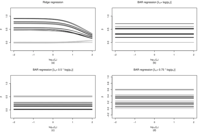
We illustrate below how the BAR estimator behaves by fixing λn and varying the tuning parameter ξn of the initial Cox ridge regression. Figure 3.1 (panels (b), (c) and (d)) depicts the solution path plots average over 100 Monte Carlo simulations of the BAR estimator with respect to ξn over a wide interval [10−2,102] for n = 300, pn = 100, ≈25% censoring, and λn = log(pn),0.5 log(pn),0.75 log(pn), respectively. The resulting BAR estimator is essentially unchanged, regardless of the choice of λn, over a large interval of ξn, suggesting that the BAR estimator is relatively insensitive to original ridge estimator.
As a reference, we also display the solution path plots of the corresponding initial ridge estimator in panel (a). The initial ridge estimator starts to introduce over shrinkage and, consequently, estimation bias when ξn exceeds 101. However, its bias has been effectively corrected by BAR. Therefore, by iteratively refitting reweighted Cox ridge regression, the BAR estimator not only performs variable selection by shrinking estimates of the true zero parameters to zero, but also effectively corrects the estimation bias from the initial Cox ridge estimator. Similar results are obtained for several different simulation scenarios and can be found in Appendix A3.5.
3.2.2 Model selection and parameter estimation
In this simulation, we evaluate and compare the variable selection and parameter estimation performance of BAR with four popular penalized Cox regression methods: LASSO (Tibshi-rani, 1997), SCAD (Fan and Li, 2002) , adaptive LASSO (ALASSO) (Zhang and Lu,2007), and MCP (Zhang,2010). We fix ξn= 1 for the BAR methods since Section 3.2.1 yields evi-dence that the BAR estimator is insensitive to the selection of ξn. BIC-score minimization is used to select the optimal tuning parameter for all five penalization methods.
Estimation bias is summarized through the mean squared bias (MSB), E(||βˆ−β0||2).
Variable selection performance is measured by a number of indices: the mean number of false positives (FP), the mean number of false negatives (FN); and average similarity measure (SM) for support recovery where SM =||S ∩ Sˆ 0||0/
q
−2 −1 0 1 2 0.0 0.5 1.0 Ridge regression log10(ξn) β (a) −2 −1 0 1 2 0.0 0.5 1.0
BAR regression [λn= log(pn)]
log10(ξn) β (b) −2 −1 0 1 2 0.0 0.5 1.0
BAR regression [λn= 0.5 * log(pn)]
log10(ξn) β (c) −2 −1 0 1 2 −0.2 0.0 0.2 0.4 0.6 0.8 1.0
BAR regression [λn= 0.75 * log(pn)]
log10(ξn)
β
(d)
Figure 3.1: Path plot for BAR regression with varying ξn and: (b) λn = log(pn), (c)
λn = 0.5 log(pn), and (d) λn = 0.75 log(pn) with estimates averaged over 100 Monte Carlo simulations of size n = 300, pn = 100, and censoring rate ≈ 25%. Path plot for ridge regression (d) with varying ξn is also included as a comparison.
of indices for the non-zero components of β0 and ˆβ, respectively (Zhang and Cheng, 2017).
The similarity measure can be viewed as a continuous measure for true model recovery: it is close to 1 when the estimated model is similar to the true model and close to 0 when the estimated model is highly dissimilar to the true model. We use the R package ncvreg
to perform LASSO, adaptive LASSO (ALASSO), SCAD, and MCP penalizations in our simulations. For ALASSO, we let the initial weight be the maximum partial likelihood estimator since pn< n. Partial simulation results are summarized in Table 3.1 where we fix
n= 300,1000,pn= 100, a censoring rate of≈25%, and average results over 100 replications. It is observed from Table 3.1 that when the tuning parameterλis selected by minimizing the BIC score as the other methods, the performance of BAR is generally comparable to other methods with respect to all measures across all scenarios. We have conducted more extensive
Table 3.1: (Moderate dimension and sample size) Simulated estimation and variable selection performance of BAR, LASSO, SCAD, ALASSO, and MCP where the BIC criterion was used to select the tuning parameters via a grid search. (MSB = mean squared bias; FN = mean number of false positives; FP = mean number of false negatives; SM = similarity measure; BIC = average BIC score; Each entry is based on 100 Monte Carlo samples of size n = 300 (top), and 1000 (bottom), pn = 100, censoring rate ≈25%.)
MSB FN FP SM BIC BAR 0.11 0.01 1.79 0.89 1919.26 LASSO 0.27 0.01 3.32 0.82 1958.40 SCAD 0.12 0.01 2.23 0.87 1933.43 ALASSO 0.11 0.04 1.48 0.90 1935.60 MCP 0.09 0.02 1.21 0.92 1929.33 BAR 0.02 0.00 0.73 0.95 8196.51 LASSO 0.10 0.00 2.77 0.84 8236.76 SCAD 0.01 0.00 0.23 0.98 8203.00 ALASSO 0.02 0.00 0.26 0.98 8204.58 MCP 0.01 0.00 0.08 0.99 8202.04
simulations with different combinations of model dimension, censoring rates, sample sizes, and model sparsity, which yielded consistent findings and are reported in Appendix A3.6
3.2.3 Sparse high-dimensional massive sample size data
In this simulation, we simulate a sHDMSS time-to-event dataset with n = 200,000 and
pn = 20,000. Event times are generated from an exponential hazards model with baseline hazardh0(t) = 1, regression coefficientsβ0 = (0.710,0.510,110,−0.710,−0.510,−110,0pn−60),
and a censoring rate of 95%. The covariates for each subject are simulated such, on average, 2% are assigned a non-zero value. The amount of memory used to store this dense design matrix would require over 16GB, which exceeds the functional capacity of most statistical software packages on standard hardware. To overcome this difficulty, we efficiently store the information in a coordinate list fashion and compare our BAR method with the mas-sive sparse Cox’s regression for LASSO (mCox-LASSO) using theCyclops package (Suchard et al., 2013; Mittal et al., 2014) which, to the best of our knowledge, is the fastest soft-ware available today that exploits the sparsity of sHDMSS time-to-event data for efficient computing and offers > 10-fold speedup (Mittal et al., 2014) over its competitors such as
Table 3.2: (Sparse high dimensional and massive sample size) Estimation and variable selec-tion results for BAR and massive Cox regression with LASSO penalty (mCox-LASSO,Mittal et al. (2014)) for a simulated sHDMSS dataset withn = 200,000,pn = 20,000, andqn = 60. (Bias = ||βˆ−β0||2; FP= number of false positives; FN = number of false negatives.)
Method Bias FP FN BIC score BAR (BIC) 0.82 5 0 226200.5 mCox-LASSO (BIC) 2.49 5 0 227059.5 mCox-LASSO (CV) 2.02 120 0 227955.3
CoxNet (Simon et al., 2011) and FastCox (Yang and Zou, 2012). For LASSO, cross vali-dation (mCox-LASSO (CV)), combined with a nonconvex optimization technique which is more efficient than the classical grid search approach, and BIC score minimization (mCox-LASSO (BIC)), implemented with the classical grid search approach, were used to find the optimal value for the tuning parameter. For the BAR method, we also implement BIC score minimization using a classical grid search. We report the bias (||βˆ−β0||2), number of false
positives (FP), false negatives (FN), and BIC score (−2ln( ˆβ) + log(n)
P
jI( ˆβj 6= 0)) in Table 3.2.
All three methods retain the 60 true nonzero coefficients; however, mCox-LASSO using cross validation selects a large number of noise variables (120) compared to BAR and mCox-LASSO using BIC minimization (5). In addition, of the five noise variables selected by both BAR (BIC) and mCox-LASSO (BIC), four of them are overlapping. In terms of parameter estimation, BAR is less biased (0.82) than mCox-LASSO (2.49 for BIC and 2.02 for CV). For model fit, BAR has a much lower BIC score when compared to the mCox-LASSO methods. In summary, this simulation illustrates that BAR produces a sparse model with less bias and better model fit compared to mCox-LASSO.
We further examined the solution paths of mCox-LASSO and BAR in Figure 3.2. The vertical solid and dashed lines in the mCox-LASSO solution path plot (Figure 3.2(a)) rep-resent the estimates at the optimal tuning parameter obtained via cross validation and BIC minimization, respectively. We can see that the mCox-LASSO solution path changes rapidly as its tuning parameter varies. In contrast, the BAR solution path plot (Figure 3.2(b)) with respect to λn changes very slowly over a relatively where the vertical line represents the