UC Irvine
UC Irvine Previously Published Works
Title
Multi-model ensemble hydrologic prediction using Bayesian model averaging
Permalink
https://escholarship.org/uc/item/8q4423c1
Journal
Advances in Water Resources, 30(5)
ISSN
0309-1708
Authors
Duan, Q
Ajami, NK
Gao, X
et al.
Publication Date
2007-05-01
DOI
10.1016/j.advwatres.2006.11.014
License
https://creativecommons.org/licenses/by/4.0/ 4.0
Peer reviewed
eScholarship.org
Powered by the California Digital Library
Multi-model ensemble hydrologic prediction using
Bayesian model averaging
Qingyun Duan
a,*, Newsha K. Ajami
b,1, Xiaogang Gao
b, Soroosh Sorooshian
baLawrence Livermore National Laboratory, P.O. Box 808, 7000 East Ave., Livermore, CA 94550, United States bUniversity of California at Irvine (UCI), Irvine, CA, United States
Received 3 July 2006; received in revised form 22 November 2006; accepted 30 November 2006 Available online 26 January 2007
Abstract
Multi-model ensemble strategy is a means to exploit the diversity of skillful predictions from different models. This paper studies the use of Bayesian model averaging (BMA) scheme to develop more skillful and reliable probabilistic hydrologic predictions from multiple competing predictions made by several hydrologic models. BMA is a statistical procedure that infers consensus predictions by weighing individual predictions based on their probabilistic likelihood measures, with the better performing predictions receiving higher weights than the worse performing ones. Furthermore, BMA provides a more reliable description of the total predictive uncer-tainty than the original ensemble, leading to a sharper and better calibrated probability density function (PDF) for the probabilistic predictions. In this study, a nine-member ensemble of hydrologic predictions was used to test and evaluate the BMA scheme. This ensemble was generated by calibrating three different hydrologic models using three distinct objective functions. These objective func-tions were chosen in a way that forces the models to capture certain aspects of the hydrograph well (e.g., peaks, mid-flows and low flows). Two sets of numerical experiments were carried out on three test basins in the US to explore the best way of using the BMA scheme. In the first set, a single set of BMA weights was computed to obtain BMA predictions, while the second set employed multi-ple sets of weights, with distinct sets corresponding to different flow intervals. In both sets, the streamflow values were transformed using Box–Cox transformation to ensure that the probability distribution of the prediction errors is approximately Gaussian. A split sample approach was used to obtain and validate the BMA predictions. The test results showed that BMA scheme has the advantage of generating more skillful and equally reliable probabilistic predictions than original ensemble. The performance of the expected BMA predictions in terms of daily root mean square error (DRMS) and daily absolute mean error (DABS) is generally superior to that of the best individual predictions. Furthermore, the BMA predictions employing multiple sets of weights are generally better than those using single set of weights.
2006 Elsevier Ltd. All rights reserved.
Keywords: Bayesian model averaging; Ensemble hydrologic prediction; Multi-model combination; Uncertainty estimation
1. Introduction
The prevailing practice by hydrologists to date has been to rely on a single hydrologic model to perform hydrologic predictions. Despite the tremendous amount of resources invested in developing more hydrologic
models, no one can convincingly claim that any particular model in existence today is superior to other models for all type of applications and under all conditions [42,43,35,3,13]. Different models have strengths in captur-ing different aspects of the hydrologic processes. Relycaptur-ing on a single model often leads to predictions that represent some phenomena or events well at the expenses of others. Further, a proper accounting of uncertainty associated with these predictions has not received adequate atten-tion. Ensemble approaches based on multi-parameter sets and ensemble hydrologic forcing inputs can help improve 0309-1708/$ - see front matter 2006 Elsevier Ltd. All rights reserved.
doi:10.1016/j.advwatres.2006.11.014
*
Corresponding author. Tel.: +1 925 4227 704; fax: +1 925 4226 388.
E-mail address:[email protected](Q. Duan).
1 Present address: Berkeley Water Center, University of California,
Berkeley, CA, United States.
the uncertainty estimation [4,20,41,23]. But the structural error inherent in any single model cannot be avoided in this kind of ensemble strategy [17]. This has motivated a number of researchers to advocate multi-model methods for hydrologic predictions [33,17,1,3].
Multi-model methods were used in various forecasting applications such as economic and weather forecasting as early as the 1960s [2,9,10,28,38]. Shamseldin and col-leagues were probably the first to explore the use of multi-model methods for hydrologic predictions [33]. Georgakakos et al.[17] recently used a multi-model com-bination approach to analyze the simulation results from multiple models that participated in the distributed model intercomparison project (DMIP) [35]. These multi-model techniques provide consensus predictions by linearly com-bining individual model predictions according to different weighting strategies. The weights can be equal for all models in the simplest case, or be determined through certain regression-based methods. In the latter case, the weights are the regression coefficients. Shamseldin and O’Connor [34] also explored the use of artificial neural network (ANN) techniques to estimate the model weights. Raftery et al. [29] pointed out that the weights determined by those regression based techniques are hard to interpret because they take on arbitrary negative or positive values and are not connected to model perfor-mance. Furthermore, the reliability of the multi-model predictions from these approaches is not satisfactory. Nevertheless, multi-model ensemble averages produced by these methods have shown to consistently perform better than single model predictions when they are evalu-ated based on various predictive skill and reliability scores [33,34,19,45,17,1].
Recently, Bayesian model averaging (BMA) has gained popularity in diverse fields such as statistics, management science, medicine and meteorology [18,40,15,29,30]. Like predictions from other multi-model methods, BMA predictions are weighted averages of the individual pre-dictions from competing models. But unlike some multi-model methods, BMA also provides a more realis-tic description of the predictive uncertainty that accounts for both between-model variances and in-model variances. The BMA weights, all positive and summing up to 1, reflect relative model performance because they are the probabilistic likelihood measures of a model being correct given the observations. In various case studies, BMA has been shown to produce more accurate and reliable predictions than other multi-model techniques Raftery et al., 1997; [8,40,31,30,14]. Recently, BMA methods have also been applied to hydrologic applica-tions such as groundwater modeling by Neuman and Wierenga [27,26].
This study explores the use of BMA for hydrologic streamflow predictions. We are interested in how BMA scheme can be used to improve both the accuracy and reliability of streamflow predictions. Particularly, we investigate different ways to apply BMA scheme to fully
exploit the strengths of individual models. This paper is organized as follows. Section 2 presents the BMA meth-odology. Section3 discusses the generation of hydrologic model ensemble and the design of the numerical experi-ments and test data sets. Section 4 describes the test and validation results of multi-model predictions using BMA schemes. Section 5 provides summaries and conclusions.
2. Bayesian model averaging (BMA)
Bayesian model averaging (BMA) is a statistical scheme to infer a probabilistic prediction that possesses more skill and reliability than the original ensemble members pro-duced by several competing models[22,29]. BMA has been used primarily in generalized linear regression applications. Recently, Raftery et al.[29,30] successfully applied BMA to dynamical modeling applications (i.e., numerical weather predictions). In this study, we apply BMA to streamflow prediction problems. The BMA scheme is briefly described as follows.
Consider a quantity y to be the forecasted variable (or predictand),D¼ ½yobs
1 ;yobs2 ;. . .;yobsT to be the training data with data lengthT, andf ¼ ½f1;f2;. . .;fKthe ensemble of all considered model predictions.pkðy jfk;DÞis the
poster-ior distribution of y given model predictionfk and
obser-vational data set D. According to the law of total probability, the probability density function (PDF) of the BMA probabilistic prediction of y can be represented as:
pðyjDÞ ¼X
K
k¼1
pðfkjDÞ pkðyjfk;DÞ ð1Þ
wherepðfkjDÞis the posterior probability of model predic-tionfk, also known as the likelihood of model predictionfk
being the correct prediction given the observational data, D. This term reflects how well this particular ensemble member matches the observations. If we denote wk¼pðfkjDÞ, we should obtain PKk¼1wk ¼1:The poster-ior mean and variance of the BMA prediction can be expressed as[29,30]: E½yjD ¼X K k¼1 pðfkjDÞ E½pkðyjfk;DÞ ¼ XK k¼1 wkfk ð2Þ Var½yjD ¼X K k¼1 wk fk XK i¼1 wifi !2 þX K k¼1 wkr2k ð3Þ wherer2
j is the variance associated with model prediction fkwith respect to observation D. In essence, the expected
BMA prediction is the average of individual predictions weighted by the likelihood that an individual model is correct given the observations. There are several attrac-tive properties to the BMA prediction. First the BMA prediction receives higher weights from better performing models as the likelihood of a model is essentially a mea-sure of the agreement between the model predictions and
the observations. Second, the BMA variance is essentially an uncertainty measure of the BMA prediction. It contains two components: the between-model-variance and the within-model-variance, as shown in the first and second terms of the right hand side of Eq (3). This measure is a better description of predictive uncertainty than that in a non-BMA scheme, which estimates uncertainty based only on the ensemble spread (i.e., only the between-model variance is considered), and conse-quently results in under-dispersive predictions Raftery et al. [29].
Before we present the BMA algorithm, it is assumed that the conditional probability distribution pkðyjfk;DÞ is Gaussian. Considering that the probability distribution of streamflow error is non-Gaussian, both modeled and observed streamflow data are pre-processed using the Box–Cox transformation prior to the BMA procedure, so that the transformed variables will be close to the Gaussian distribution. The Gaussian assumption is made for compu-tational convenience and BMA scheme can be applied by assuming other probability distributions. Statistical tech-niques such as Markov Chain Monte Carlo (MCMC) method is capable of simulating any complex probability distribution, therefore, can be a strategy to conduct BMA without using the Gaussian approximation[21]. However, it is beyond the focus of this paper. We will work with the log-likelihood function since it is more convenient to compute than the likelihood function itself. If we denote
h¼ ½fwk;rk;k¼1;2;. . .;Kg, the log-likelihood function can be approximated as:
‘ðhÞ ¼log X K k¼1 wkpkðyjfk;DÞ ! ð4Þ
Obviously, it is impossible to obtain analytical solution ofhand an iterative procedure must be used. Following the recommendation of Raftery et al.[30], we used the Expec-tation–Maximization (EM) algorithm for this purpose. In brief, the EM algorithm casts the maximum likelihood problem as a ‘‘missing data’’ problem. The missing data may not be actual data. Rather, it can be a latent variable that needs to be estimated. For this study, a latent variable zk;tis introduced. If thekth model ensemble is the best pre-diction at timet,zk;t¼1; otherwisezk;t¼0. At any timet, there is only onezk;tequal to 1 and the rest is equal to 0. As in the namesake, the EM algorithm alternates between the E (or expectation) step and the M (or maximization) step. It starts with an initial guess,hð0Þ, for parameterh. In the E step,zk;tis estimated given the current guess ofh. In the M step,his estimated given the current values of thezk;t. The
EM steps are repeated until certain convergence criteria are satisfied. The EM algorithm is illustrated in Box 1. The EM algorithm can only find local optimum and the optimal solution is very sensitive to initial guess of the optimizing variables. For a more detailed description of the EM algo-rithm, readers are referred to McLachlan and Krishnan [24].
Box 1: EM Algorithm A. Initialization: Set Iter¼0;wIterk ¼1
K;r 2ðIterÞ k ¼ 1 K XT t¼1 PK k¼1ðytfk;tÞ 2 T whereTis the total number of data points in the training period
B. Computing the initial likelihood:
‘ðhIterÞ ¼log X K k¼1 wkpkðyjfk;DÞ ! ¼log X K k¼1 wk XT t¼1 g yobst jfk;t;rð IterÞ k ! ðB1Þ
whereg(.) denotes Gaussian distribution. C. Executing the expectation step
SetIter¼Iterþ1.
Fork¼1;2;. . .;K, and t¼1;2;. . .;T, compute:
^ zIterk;t ¼ g ytjfk;t;r ðIter1Þ k PK k¼1gðyobst jfk;t;rð Iter1Þ k Þ ðB2Þ
D. Executing the maximization step Compute the weight;wIter
k ¼ 1 T XT t¼1 zIter k;t ðB3Þ
Update the variance;r2ðIterÞ
k ¼ PT t¼1^zIterk;t yobst fk;t 2 PT t¼1^zIterk;t ðB4Þ
Update the likelihood using Eq(B1). E. Checking convergence:
If‘ðhIterÞ ‘ðhIter1Þis less than or equal to a pre-specified tolerance level, stop; else go back to Step C.
With proper estimate of h¼ ½fwk;rk;k¼1;2;. . .;Kg andpkðyjfk;h;DÞ, we can easily generate probabilistic pre-dictions based on Eq.(1). An algorithm to generate BMA probabilistic predictions is presented later in Section4.3.2.
3. Generation of hydrologic model ensemble
To test BMA scheme for streamflow predictions, an ensemble of competing predictions from several hydrologic models were produced. For this study, we employed three conceptual hydrologic models: the Sacramento Soil Mois-ture Accounting (SAC-SMA) model, the Simple Water
Balance (SWB) model, and the HYMOD model. SAC-SMA is the most complicated model among the three, with 16 model parameters, and is still the most widely used oper-ational hydrologic model in Noper-ational Weather Service for river and flood forecasting purpose [7]. SWB, also devel-oped by NWS, is a simple hydrologic model used operation-ally in the Nile River Forecast System in Egypt [32]. HYMOD is a simple hydrologic model developed for research purposes at the University of Arizona [5]. Both SWB and HYMOD have five tunable model parameters. All three models need precipitation and potential evapo-transpiration data as forcing inputs. A detailed description of these individual models is outside the scope of this paper. Interested readers should refer appropriate literature to gain a more in-depth understanding of these models.
The three hydrologic models were calibrated using the Shuffled Complex Evolution method (SCE-UA, [11,12]. Three distinct objective functions were used to force the hydrologic models to favor different phases of the hydrograph:
• Daily root mean square error (DRMS),
• Daily absolute error (DABS)
• Heteroscedastic maximum likelihood estimator (HMLE)
The analytical expressions of these objective functions are: DRMS¼ ffiffiffiffiffiffiffiffiffiffiffiffiffiffiffiffiffiffiffiffiffiffiffiffiffiffiffiffiffiffiffiffiffiffiffiffi PT t¼1 yobst yestt 2 T s ð5aÞ DABS¼ PT t¼1 y obs t y est t T ð5bÞ HMLE¼ PT t¼1xt yobst y est t 2 ffiffiffiffiffi QT t¼1 T s xt ð5cÞ whereyobs t andy est
t are observed and estimated streamflow values,xt¼f
2ðk1Þ
t andk is the unknown Box–Cox trans-formation parameter [36]. The first objective function, DRMS, forces the models to fit the high flows well, while the last objective function, HMLE, tends to push the
models to match low flows well. The second objective function, DABS, places equal emphasis on all parts of the hydrograph and is a compromise between DRMS and HMLE.
We carried out hydrologic model calibration on three hydrologic basins located in the United States: Bird Creek River basin, near Sperry, OK; Leaf River basin, Near Collins, MS; and French Broad River basin at Blantyre, NC. These basins are chosen because they have been widely studied and the hydrologic data sets were carefully prepared by NWS Hydrology Laboratory [37,32]. Table 1lists the geophysical and climatic charac-teristics of these test basins. The hydrologic data periods for these basins are also shown. These basins span differ-ent hydroclimatic regimes, from semi-arid (e.g., Bird Creek), to moderate (e.g., Leaf River), and to wet (e.g., French Broad River).
The combination of three models and three objective functions yields a nine-member ensemble of distinct model predictions for each test basin. This ensemble forms the basis for testing the BMA scheme in the next sections. Table 2summarizes the DRMS statistics over the calibra-tion period for each ensemble member in different flow intervals for the test basins. The entire flow range was broken into a number of flow intervals based on pre-spec-ified non-exceedance threshold (e.g., 10%, 25%, 50%, 75%, 90%, 100%). As expected, different ensemble members exhibit different goodness-of-fit statistics in different flow intervals, with the SAC-SMA as an obviously better model among the three in most cases. It is worth noting that, with a few exceptions, the ensemble members cali-brated using DRMS tend to be associated with better sta-tistics at the high flow ranges, while the ensemble members calibrated using HMLE generally correspond to better statistics in the low flow ranges. The ensemble members calibrated with DABS tend to favor the mid-dle-ranges.
A necessary condition for obtaining unbiased, optimal results using the BMA scheme, as outlined in 2, is that the likelihood function of the prediction error must be properly computed. In this study, we employed a likeli-hood function that assumes the underlying variable is normally distributed for computational simplicity. It is
Table 1
Geophysical and climatic characteristics of the test basins Basin name
Bird Creek Leaf River French Broad
Location Sperry, OK Collins, MS Blantyre, NC
Latitude 361604200 314202500 351705700
Longitude 955701400 892402500 823702600
Area, km2 2344 1924 766
Ann. precip, mm 963 1313 1878
Ann. runoff, mm 220 428 1080
Ann. pot. evap., mm 1312 1310 1159
Data period 10/1/1955–9/30/1962 10/1/1951–9/30/1969 10/1/1953–9/30/1964
Training/calib. period 1/1/1956–9/30/1960 10/1/1952–9/30/1960 1/1/1953–9/30/1958
well known that the error in streamflow prediction is het-eroscedastic and non-Gaussian [36,39]. To deal with this problem, we performed a Box–Cox transformation on streamflow values prior to BMA testing to ensure that the streamflow prediction error is approximately Gaussian.
In the following section, we carried out several numer-ical experiments to assess the usefulness of BMA scheme for streamflow prediction. Particularly, the BMA scheme was evaluated using two strategies. In the first strategy, we applied the BMA scheme to obtain a single set of BMA weights for the entire Box–Cox transformed time series. In the second strategy, we break the Box–Cox transformed streamflow values into several flow ranges and then apply the BMA scheme to each flow range sep-arately. There is an intuitive advantage to using a multi-flow interval approach: the strengths of individual models in capturing different aspects of the hydrographs (i.e., peak flows and low flows) are reflected in the computa-tion of the model weights. A model that predicts high peak flows better than other models would be assigned a higher weight than other models during peak flow peri-ods. Reversely, a model that represents low flow better would also be given a higher weight during the low flow periods.
The results presented below seek to answer the following questions: (1) how do we exploit the diversity in skill levels of different predictions over different flow periods? (2) will the BMA weights as defined in Eqs. (2)–(4) reflect the model performance statistics? (3) how consistent are the BMA predictions when the BMA weights obtained from the training periods are applied to independent validation periods?
4. Results
4.1. Statistical verification criteria
Before the results from the numerical experiments are presented, we first define the criteria used to evaluate the performance of model predictions. For hydrologic predictions, the common goals are to maximize the pre-dictive accuracy and reliability. There are many ways to measure these goals. In this study, we employed a number of criteria: DRMS and DABS (as defined in the previous section), Ranked Probability Score (RPS) and Reliability Diagram (REL). DRMS and DABS are commonly used for evaluating the accuracy of deterministic predictions and they are used here to evaluate the association of the expected BMA predictions with observations. For probabilistic predictions, it is desired that the probability density function (PDF) is sharp subject to calibration. By ‘‘calibration’’, it means that the PDFs of the predictions and observations are consistent. RPS and REL are widely used as measures for assessing the quality of probabilistic predictions. RPS is essentially the mean-squared error of the probability forecasts averaged over multiple events. A small value for RPS means that the PDF is sharp and well calibrated. In streamflow prediction, the proba-bility forecast is often expressed as a non-exceedance probability forecast in pre-specified categories (i.e., 5%, 10%, 25%, 50%, 75%, 90%, 95% 100% non-exceedance). The observed value for a given forecast category takes on the value of 1 if the observed flow value is less than the threshold for that category. Otherwise, the observed value is 0. The analytical expression of RPS for an event is given as:
Table 2
DRMS statistics of individual ensemble members during calibration period Flow ranges, mm/day,
(% quantile)
SAC SWB HYM
DRMS DABS HMLE DRMS DABS HMLE DRMS DABS HMLE
Bird Creek 0–0.04 (0–50%) 0.2335 0.0334 0.0193 0.0935 0.0831 0.0324 0.2737 0.1577 0.1320 0.04–0.2 (50–75%) 0.4279 0.1474 0.1666 0.2705 0.2279 0.3562 0.4036 0.2510 0.2882 0.2–0.93 (75–90%) 0.7211 0.5137 0.5866 1.027 1.0531 1.2133 0.6098 0.3642 1.0487 0.93–64 (90–100%) 2.0965 2.6613 3.0749 2.6253 2.7281 6.3026 2.8133 3.3268 4.3429 Overall 0.7433 0.8505 0.9828 0.9055 0.9346 2.0166 0.9403 1.0553 1.4089 Leaf River 0–0.12 (0–10%) 0.0743 0.0441 0.0292 0.1016 0.1004 0.0860 0.0821 0.0442 0.0188 0.12–0.17 (10–25%) 0.1045 0.0585 0.0344 0.1579 0.1326 0.0966 0.1325 0.0873 0.0281 0.17–0.35 (25–50%) 0.1734 0.1132 0.0713 0.2622 0.2624 0.2149 0.2818 0.2168 0.0799 0.35–0.97 (50–75%) 0.4193 0.3088 0.2698 0.5499 0.5341 0.4296 0.5198 0.4130 0.2642 0.97–2.78 (75–90%) 0.8291 0.7150 0.9194 1.0961 0.8275 0.8481 0.8037 0.7012 0.9986 2.78–58 (90–100%) 2.2672 2.5400 2.8709 2.5171 3.0363 4.0484 2.9221 3.1897 4.4993 Overall 0.8358 0.8870 1.0093 0.9728 1.0814 1.3800 1.0428 1.0975 1.5206 French Broad 0–0.94 (0-10%) 0.2201 0.2225 0.1854 0.3731 0.2759 0.2347 0.2489 0.26 0.2465 0.94–1.47 (10–25%) 0.3152 0.3065 0.2561 0.4801 0.4212 0.3623 0.4801 0.4766 0.5068 1.47–2.36 (25–50%) 0.4168 0.4293 0.3792 0.6694 0.6125 0.6279 0.6426 0.5995 0.7503 2.36–3.6 (50–75%) 0.5221 0.5246 0.4712 0.9323 0.8452 0.8294 0.7629 0.7564 0.9703 3.6–5.39 (75–90%) 0.8801 0.7979 0.7223 1.1931 1.2038 1.1328 1.1391 1.1989 1.4745 5.39–53 (90–100%) 1.5227 1.6633 1.9693 2.2929 2.576 2.7719 2.2799 2.3146 2.7223 Overall 0.6556 0.6724 0.7085 1.0033 1.0277 1.0533 0.9471 0.9564 1.1524
RPSðtÞ¼X M j¼1 FðjtÞOðjtÞ 2 ð6Þ
where FðjtÞ is the forecast probability and OðjtÞ is the ob-served value, j¼ f1;2;. . .;Mg is the probability category andt is the event index. Here, we treat the flow value for each day as an event. The average RPSðtÞ over an evalua-tion periodt¼ f1;2;. . .;Tgis equal to the overall RPS:
RPS¼1
T
XT t¼1
RPSðtÞ ð7Þ
Reliability diagram (REL) measures how the forecast probability matches observation for all forecast categories. In probability term, REL is the conditional distribution of an observation given a particular forecast,pðOjFÞ. A per-fect forecast impliespðO¼1jFÞ ¼F. We will explain the interpretation of REL later when we present the results. For a more general discussion on verification statistics, readers are referred to Murphy et al. [25,44]. For a more detailed discussion on verification of probabilistic hydro-logic forecast, readers are referred to Franz et al., Bradley et al.[16,6].
Verification statistics such as DRMS, DABS and RPS, are not meaningful when they are viewed in absolute terms. That is why skill scores are used widely in verification liter-ature [25,44]. Skill scores, DRMSS, DABSS, and RPSS, are usually computed as the percentage improvement over a reference point: DRMSS¼ 1 DRMS DRMS 100 ð8aÞ DABSS¼ 1DABS DABS 100 ð8bÞ RPSS¼ 1RPS RPS 100 ð8cÞ
where DRMS, DABS, and RPS are the verification statistics of a prediction, and DRMS, DABS, and RPS are the reference verification statistics. In this study, DRMS and DABS are the verification statistics associated with the best individual prediction among the original ensemble, while RPS is the RPS value com-puted from the original ensemble. Note that for skill scores, the larger the values, the better are the predictions.
4.2. Box–Cox transformation of streamflow values
Before we applied the BMA scheme as described in Sec-tion 2 to the nine-member ensemble shown in Table 2, a Box–Cox transformation was first performed on both the ensemble members and the observation. The Box–Cox transformation is given as follows:
zt¼ yk t1 k ; k6¼0 logðytÞ; k¼0 ( ð9Þ
where yt is the original variable, zt is the transformed
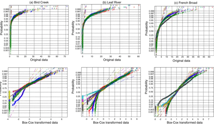
variable, k is the Box–Cox coefficient. For each basin, we derived a common optimal estimate of k for all ensemble members and the observations, based on Kol-mogorov–Smirnov test statistics. Fig. 1 displays the nor-mal probability plots of the original and transformed ensemble members. It is clear that the original ensemble members are highly non-Gaussian, while the transformed members appear much closer to be normally distributed. Still we notice that a few transformed ensemble members depart from the Gaussian distribution at the lower tail end.
4.3. Testing of BMA scheme using a single set of weights 4.3.1. Verification of the accuracy of the expected BMA predictions obtained using a single set of BMA weights
The BMA scheme was applied to the transformed ensemble members to obtain a single set of BMA weights for each basin using all data points from the training per-iod. The weights for different ensemble members are shown in Fig. 2. Before we examine the BMA weights, let’s first look at the performance statistics of the expected BMA predictions (denoted as BMA1 predictions hereafter),
which are really alternative deterministic predictions to the individual predictions. Note that all statistics were computed on streamflow values in original space (not the Box–Cox transformed space). The DRMSS and DABSS statistics of the expected BMA1 predictions, along with
that of the simple model average (SMA) predictions, are shown inFig. 3a and b.Fig. 3a shows that the DRMSS sta-tistics of the expected BMA1 predictions are better than
that of the best individual predictions, substantially in the cases of Bird Creek and French Broad. In terms of the DABSS statistics, the BMA1predictions are slightly better
than the best individual prediction in Bird Creek basin. But in two other basins, the DABSS statistics of BMA1
predic-tions are slightly worse than the best individual predicpredic-tions (Fig. 3b). Compared to the best individual predictions, SMA predictions generally performed much worse than the best individual predictions, except in one basin (i.e., Bird Creek). This indicates that simply averaging the origi-nal ensemble predictions would not necessarily lead to improved accuracy of the predictions.
One premise of the BMA scheme is that BMA weights should reflect relative model performance. From Fig. 2, we quickly notice visually that, indeed, individual model performance roughly reflects the BMA weights, with SAC model weighed more heavily than other models. The corre-lation coefficients between the BMA1 weights and the
DRMS and DABS statistics were computed for each basin and were shown inTable 3. All of these correlation coeffi-cients have high negative values, indicating that higher weights are strongly associated with lower DRMS and DABS values. This confirms that the BMA weights do indeed reflect model performance.
0 10 20 30 40 50 60 70 0.001 0.003 0.01 0.02 0.05 0.10 0.25 0.50 0.75 0.90 0.95 0.98 0.99 0.997 0.999 0.001 0.003 0.01 0.02 0.05 0.10 0.25 0.50 0.75 0.90 0.95 0.98 0.99 0.997 0.999 0.001 0.003 0.01 0.02 0.05 0.10 0.25 0.50 0.75 0.90 0.95 0.98 0.99 0.997 0.999 0.001 0.003 0.01 0.02 0.05 0.10 0.25 0.50 0.75 0.90 0.95 0.98 0.99 0.997 0.999 Original data Probability Probability Probability 0.001 0.003 0.01 0.02 0.05 0.10 0.25 0.50 0.75 0.90 0.95 0.98 0.99 0.997 0.999 Probability Probability 0.001 0.003 0.01 0.02 0.05 0.10 0.25 0.50 0.75 0.90 0.95 0.98 0.99 0.997 0.999 Probability
(a) Bird Creek
-4 -2 0 2 4 6
Box-Cox transformed data Box-Cox transformed data Box-Cox transformed data
0 10 20 30 40 50 60
Original data Original data
(b) Leaf River
-3 -2 -1 0 1 2 3 4 5 6
0 5 10 15 20 25 30 35 40 45 50
(c) French Broad
-3 -2 -1 0 1 2 3 4 5 6 7
Fig. 1. Normal probability plots of the original and Box–Cox transformed ensembles.
0 0.05 0.1 0.15 0.2 0 0.05 0.1 0.15 0.2 0 0.05 0.1 0.15 0.2
(a) Bird Creek
W eigh t (b) Leaf River W eigh t
SAC 1 SAC 2 SAC 3 SWB1 SWB2 SWB3 HYM1 HYM2 HYM3 SAC 1 SAC 2 SAC 3 SWB1 SWB2 SWB3 HYM1 HYM2 HYM3 SAC 1 SAC 2 SAC 3 SWB1 SWB2 SWB3 HYM1 HYM2 HYM3
(c) French Broad River
W
eigh
t
4.3.2. Verification of the skill and reliability of the BMA1
probabilistic predictions
One feature of the BMA scheme is that it can derive probabilistic ensemble predictions from competing individ-ual deterministic predictions. Box 2 briefly describes how the BMA probabilistic ensemble predictions are generated (see also [30]. For this study, we generated 100 BMA ensemble predictions to get a reasonable empirical PDF at each time step.
Box 2: Procedure for generateng BMA probabilistic ensemble predictions
(0) Select the ensemble size,M. Sett¼1. (1) Generate an integer value ofkfrom the
numbers½1;. . .;Kbased on probability
½w1;. . .;wK.
(2) Generate a value ofytfrom PDFgkðytjfk;tÞ. (3) Repeat Steps (1) and (2) M times.
(4) Sett¼tþ1. If treaches T, stop; else go to Step (1).
Fig. 4 displays the expected BMA1 predictions along
with the 90% confidence interval of the BMA1 ensemble
for one typical calendar year for each of the test basins. The corresponding observations are shown as dots. To putFig. 4in a proper perspective, we also show the corre-sponding SMA predictions along the 90% confidence inter-val of the original ensemble spread inFig. 5.Fig. 6shows that the RPSS statistics. This figure clearly indicates that theRPSvalues of BMA1predictions are significantly
bet-ter (>30%) than that of the original ensemble predictions. This implies that the PDFs of the BMA1 predictions are
sharper and more consistent with the observations than that of the original ensemble predictions. Therefore, the BMA1predictions are much more skillful than the original
ensemble.
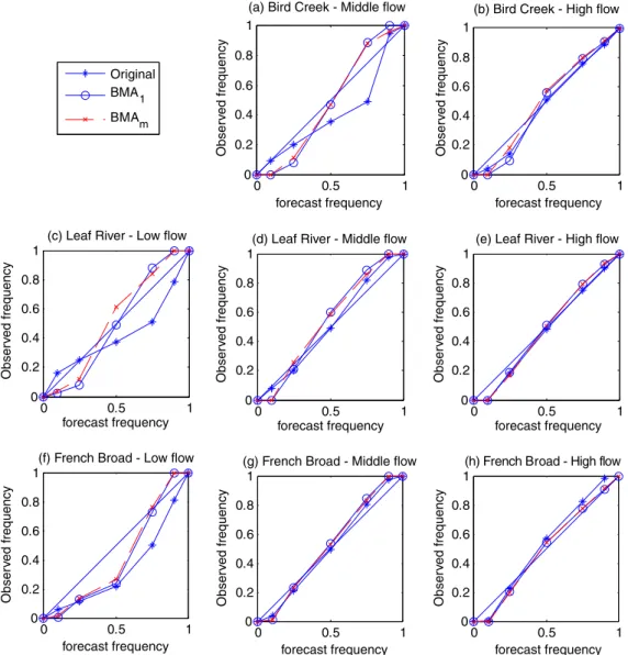
Fig. 7shows the reliability diagram of the BMA1
predic-tions and the original ensemble predicpredic-tions for three flow ranges: low flow (i.e., bottom 25% quantile based on obser-vations), middle flow (i.e., middle 50% quantile) and high flow (i.e., top 25% quantile). The reliability of the BMAm
predictions is also included in the figure. We will discuss the reliability results in Section4.4.2.
4.4. Testing of BMA scheme using multiple sets of weights In previous section, the BMA scheme was applied to the entire Box–Cox transformed time series. In this sec-tion, we broke the streamflow values from the training data period into several flow intervals. We then applied BMA scheme to each flow range and obtain a distinct set of weights for each flow range. The BMA predictions for each flow range were computed individually using the BMA weights corresponding to that particular flow range. Afterwards, the BMA predictions for different flow ranges were combined to obtain the BMA predic-tion for the entire training data period. In the following sections, the verification statistics were again computed in the original space (i.e., not in the Box–Cox trans-formed space).
4.4.1. Verification of the accuracy of the expected BMA probabilistic predictions obtained using multiple sets of weights
The streamflow values were broken into several flow ranges based on non-exceedance thresholds, as explained in Section 2. For this study, the flow range values for Leaf River and French Broad basins correspond to 10%, 25%, 50%, 75%, 90% and 100% non-exceedance levels for each basin. Because about 23% of the stream-flow values for Bird Creek basin take on the value of 0, the flow ranges for this basin correspond to 50%, 75%, 90% and 100%. For each flow range, we used the BMA scheme to estimate a distinct set of BMA weights. Bird Creek Leaf River French Broad Bird Creek Leaf River French Broad
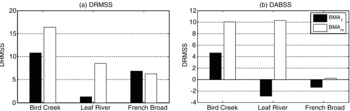
-30 -20 -10 0 10 20 (a) DRMSS DRMSS -40 -30 -20 -10 0 10 (b) DABSS DABSS SMA BMA 1
Fig. 3. DRMSS and DABSS statistics of SMA and BMA1predictions.
Table 3
The correlation coefficients between BMA weights and DRMS and DABS statistics
DRMS DABS
Bird Creek 0.88 0.91
Leaf River 0.92 0.93
Fig. 8 displays the BMA weights for all flow ranges and all basins. For some flow ranges, there is a large variabil-ity in BMA weights. For other flow ranges, the BMA weight variability is muted. The weights for SAC models are generally higher in most flow ranges. Table 4 shows the values of correlation coefficients between BMA weights and DRMS and DABS statistics averaged over different flow ranges for each basin. These high correla-tion values re-affirm the previous finding in Seccorrela-tion 4.3 that BMA weights do reflect model performance.
Now let’s evaluate the DRMSS and DABSS statistics of the combined BMA predictions obtained using multi-ple sets of weights (denoted as BMAm predictions
hereaf-ter). Fig. 9exhibits the DRMSSand DABSS statistics of both the BMA1 and BMAm predictions. This figure
indi-cates that the BMAmpredictions not only improve on the
best individual predictions, but also do better than the
BMA1 predictions in terms of DRMSS and DABSS
sta-tistics. This tells us that there is a potential advantage in using multiple weight sets over a single set of values. This probably indicates that BMAm predictions are more
capable of taking advantages of the diversity of the ensemble members.
4.4.2. Verification of the skill and reliability of the BMAm
probabilistic predictions
Using the procedure described in Box 2, we again created 100-member BMAm ensemble predictions for
each flow range using the associated BMAm weights.
The combined BMAm predictions for all flow ranges
are shown in Fig. 10, along with the 90% confidence interval. Again, the 90% confidence interval seems to encompass the observed very well. Fig. 11 shows the
0 50 100 150 200 250 300 350 0 20 40 60 Year - 1959 mm/da y
(a) Bird Creek 90% conf. int. observations expected BMA1 0 50 100 150 200 250 300 350 0 5 10 15 20 Year - 1957 mm/da y (b) Leaf River 0 50 100 150 200 250 300 350 0 10 20 30 40 Year - 1957 mm/da y (c) French Broad
RPSS statistics for the BMA predictions using both the single-set weights and multi-set weights. The RPSS sta-tistics for BMAm predictions indicates that BMAm
pre-dictions are significantly more skillful and reliable than the original ensemble predictions. But the RPSS statis-tics of BMAm and BMA1 predictions is essentially the
same.
The reliability diagram of BMAm predictions is shown
in Fig. 7, along with that of the BMA1 and original
ensemble predictions. Based on Fig. 7, the reliability of all three sets of ensemble predictions is comparable. All of the ensemble predictions have good resolution, as indi-cated by the full coverage of the observed probability range by all predictions. The reliability is excellent for some middle flow and all high flow ranges, as indicated by the reliability curves closely wrapped around the 45
line. The high reliability score is probably due to the fact
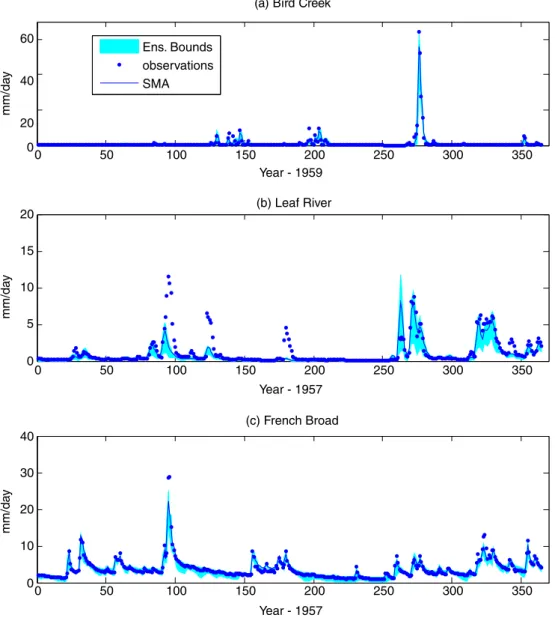
Ens. Bounds observations SMA 0 50 100 150 200 250 300 350 0 20 40 60 Year - 1959 mm/da y
(a) Bird Creek
0 50 100 150 200 250 300 350 0 5 10 15 20 Year - 1957 mm/da y (b) Leaf River 0 50 100 150 200 250 300 350 0 10 20 30 40 Year - 1957 mm/da y (c) French Broad
Fig. 5. SMA predictions and original ensemble spread.
Bird Creek Leaf River French Broad 0 5 10 15 20 25 30 35 40 45 50 RPSS
that all of the streamflow predictions have been cali-brated to observed streamflow data. The reliability for the low flow ranges is not as good as in the high flow ranges. In these low flow cases, the original ensemble pre-dictions tend to have an over-prediction bias. The reli-ability of the two BMA ensemble predictions is similar and they all tend to over-predict the low end and under-predict the high end of each flow range. Note that the low flow reliability diagram for Bird Creek is not shown. This is because almost all of the observed and predicted flow values in the low flow range are equal to 0. Note also that the reliability diagram of the middle flow range for Bird Creek is similar to that of low flow range for the two other basins.
4.5. Validation of BMA predictions using data from independent periods
The previous sections show that the BMA scheme is a promising tool for generating probabilistic predictions. A
natural question to ask is how robust are these results. In this section, we designed a set of experiments to eval-uate how the BMA predictions perform when they are evaluated using data from an independent validation period.
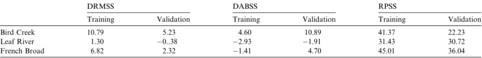
The validation periods for the test basins are listed in the last row of Table 1. We used the weights obtained from the training periods and computed BMA predic-tions for the validation periods. The performance statis-tics, including DRMSS, DABSS, RPSS and Reliability Diagrams, are again employed to examine the consistency of the BMA predictions. Table 5 lists these statistics for the training and validation periods for BMA1
predic-tions, while Table 6 provides the same information for BMAm predictions. In terms of the DRMSS statistics,
the performance of both BMA1 and BMAm predictions
in the validation period is degraded somewhat from that in the training period. The DABSS statistics indicates a mixed picture: the performance of both BMA1 and
BMAm predictions in the validation period is shown to
0 0.5 1 0 0.2 0.4 0.6 0.8 1
(a) Bird Creek - Middle flow
Original BMA1 BMAm 0 0.5 1 0 0.2 0.4 0.6 0.8 1
(b) Bird Creek - High flow
0 0.5 1 0 0.2 0.4 0.6 0.8 1
(c) Leaf River - Low flow
0 0.5 1 0 0.2 0.4 0.6 0.8 1
(d) Leaf River - Middle flow
0 0.5 1 0 0.2 0.4 0.6 0.8 1
(e) Leaf River - High flow
0 0.5 1 0 0.2 0.4 0.6 0.8 1
(f) French Broad - Low flow
Obser v ed frequency forecast frequency Obser v ed frequency forecast frequency Obser v ed frequency forecast frequency Obser v ed frequency forecast frequency Obser v ed frequency forecast frequency Obser v ed frequency forecast frequency Obser v ed frequency forecast frequency Obser v ed frequency forecast frequency 0 0.5 1 0 0.2 0.4 0.6 0.8 1
(g) French Broad - Middle flow
0 0.5 1 0 0.2 0.4 0.6 0.8 1
(h) French Broad - High flow
be improved over that in the training period for two basins (i.e., Bird Creek and French Broad) and the reverse is true for Leaf River. In terms of RPSS statis-tics, both sets of BMA predictions are still much better than the original ensemble. For Leaf River and French Broad basins, there is not much difference in RPSS sta-tistics between training and validation periods. For Bird
SAC1 SAC2 SAC3 SWB1 SWB2 SWB3 HYM1 HYM2 HYM3
SAC1 SAC2 SAC3 SWB1 SWB2 SWB3 HYM1 HYM2 HYM3
SAC1 SAC2 SAC3 SWB1 SWB2 SWB3 HYM1 HYM2 HYM3
SAC1 SAC2 SAC3 SWB1 SWB2 SWB3 HYM1 HYM2 HYM3
SAC1 SAC2 SAC3 SWB1 SWB2 SWB3 HYM1 HYM2 HYM3 SAC1 SAC2 SAC3 SWB1 SWB2 SWB3 HYM1 HYM2 HYM3 SAC1 SAC2 SAC3 SWB1 SWB2 SWB3 HYM1 HYM2 HYM3 SAC1 SAC2 SAC3 SWB1 SWB2 SWB3 HYM1 HYM2 HYM3 SAC1 SAC2 SAC3 SWB1 SWB2 SWB3 HYM1 HYM2 HYM3
SAC1 SAC2 SAC3 SWB1 SWB2 SWB3 HYM1 HYM2 HYM3 SAC1 SAC2 SAC3 SWB1 SWB2 SWB3 HYM1 HYM2 HYM3
SAC1 SAC2 SAC3 SWB1 SWB2 SWB3 HYM1 HYM2 HYM3
SAC1 SAC2 SAC3 SWB1 SWB2 SWB3 HYM1 HYM2 HYM3
SAC1 SAC2 SAC3 SWB1 SWB2 SWB3 HYM1 HYM2 HYM3
SAC1 SAC2 SAC3 SWB1 SWB2 SWB3 HYM1 HYM2 HYM3
SAC1 SAC2 SAC3 SWB1 SWB2 SWB3 HYM1 HYM2 HYM3 0 0.05 0.1 0.15 0.2 w Bird Creek 0 0.1 0.2 0.3 0.4 w 0 0.05 0.1 0.15 0.2 w 0 0.05 0.1 0.15 0.2 w 0 0.1 0.2 0.3 0.4 w Leaf River 0 0.1 0.2 0.3 0.4 w 0 0.1 0.2 0.3 0.4 w 0 0.05 0.1 0.15 0.2 w 0 0.05 0.1 0.15 0.2 w 0 0.05 0.1 0.15 0.2 w 0 0.05 0.1 0.15 0.2 w French Broad 0 0.05 0.1 0.15 0.2 w 0 0.05 0.1 0.15 0.2 w 0 0.05 0.1 0.15 0.2 w 0 0.05 0.1 0.15 0.2 w 0 0.05 0.1 0.15 0.2 w a e k l m n o p f g h i j b c d
Fig. 8. BMA weights for different flow ranges.
Table 4
Correlation coefficients between BMA weights and DRMS and DABS statistics averaged over different flow ranges
DRMS DABS
Bird Creek 0.7930 0.8878
Leaf River 0.8285 0.8543
French Broad 0.8243 0.8123
Bird Creek Leaf River French Broad Bird Creek Leaf River French Broad 0 5 10 15 20 (a) DRMSS DRMSS DRMSS -4 -2 0 2 4 6 8 10 12 (b) DABSS BMA1 BMAm
Creek, the RPSS statistics for the validation period is about half of the training period. The results here indi-cate that there is some degradation in performance when the weights generated from the training period are used for the validation period. However, the advantage of using BMA approach is still obvious compared to the bench marks used (i.e., the best individual predictions and the original ensemble).
Fig. 12 shows the reliability diagrams for the low, middle and high flow ranges (as defined in Section 4.3.2) for all three basins. The reliability of all three sets of ensemble predictions is very good and there is no degradation in terms of reliability measure between the validation and calibration period for the test basins. 90% conf. int. observations expected BMAm 0 50 100 150 200 250 300 350 0 20 40 60 Year - 1959 mm/da y
(a) Bird Creek
0 50 100 150 200 250 300 350 0 5 10 15 20 Year - 1957 mm/da y (b) Leaf River 0 50 100 150 200 250 300 350 0 10 20 30 40 Year - 1957 mm/da y (c) French Broad
Fig. 10. Expected BMAmpredictions and 95% confidence interval compared to observation.
Bird Creek Leaf River French Broad
0 10 20 30 40 50 RPSS BMA 1 BMA m
0 0.5 1 0 0.2 0.4 0.6 0.8 1
(a) Bird Creek - Middle flow
Original BMA1 BMAm 0 0.5 1 0 0.2 0.4 0.6 0.8 1
(b) Bird Creek - High flow
0 0.5 1 0 0.2 0.4 0.6 0.8
1(c) Leaf River - Low flow
0 0.5 1 0 0.2 0.4 0.6 0.8 1
(d) Leaf River - Middle flow
0 0.5 1 0 0.2 0.4 0.6 0.8 1
(e) Leaf River - High flow
0 0.5 1 0 0.2 0.4 0.6 0.8 1
(f) French Broad - Low flow
Obser v ed frequency forecast frequency Obser v ed frequency forecast frequency Obser v ed frequency forecast frequency Obser v ed frequency forecast frequency Obser v ed frequency forecast frequency Obser v ed frequency forecast frequency Obser v ed frequency forecast frequency Obser v ed frequency forecast frequency 0 0.5 1 0 0.2 0.4 0.6 0.8 1
(g) French Broad - Middle flow
0 0.5 1 0 0.2 0.4 0.6 0.8 1
(h) French Broad - High flow
Fig. 12. Reliability diagrams of BMA1and BMAmpredictions for the validation periodsTable 1. Geophysical and climatic characteristics of the test
basins. Table 5
Comparison of verification statistics between the training period and validation period for BMA1predictions
DRMSS DABSS RPSS
Training Validation Training Validation Training Validation
Bird Creek 10.79 5.23 4.60 10.89 41.37 22.23
Leaf River 1.30 0..38 2.93 1.91 31.43 30.72
French Broad 6.82 2.32 1.41 4.70 45.01 36.04
Table 6
Comparison of verification statistics between the training period and validation period for BMAmpredictions
DRMSS DABSS RPSS
Training Validation Training Validation Training Validation
Bird Creek 16.37 5.68 10.05 13.78 41.77 19.15
Leaf River 8.56 0.03 10.28 0.91 33.76 30.25
5. Summary and conclusions
All models are imperfect representations of the real-world processes. Different models have strengths in captur-ing different aspects of the real world processes. It is highly desirable that some kind of consensus predictions can take advantage of the diverse skills in different individual pre-dictions. BMA scheme has shown to be a useful statistical scheme that generates probabilistic predictions from differ-ent competing predictions. This is accomplished through a weighting strategy based on the likelihood of an individual prediction being correct given the observations. We have illustrated how the BMA scheme can be used to generate probabilistic hydrologic predictions from several compet-ing individual predictions. Here are the major findcompet-ings of this study.
(1) The expected BMA1predictions obtained by using a
single set of weights computed over the entire training period are better than or comparable to the best indi-vidual predictions in terms of DRMSS and DABSS statistics. The advantage of BMA1 predictions over
the original ensemble predictions is very significant, by 30% or better. In Leaf River, the DRMSS and DABSS scores is relatively weak, indicating that the advantage of BMA approach can be limited in cer-tain cases.
(2) The use of multiple sets of BMA weights to generate BMAmpredictions was a way to accentuate strengths
of individual models in capturing different phases of the hydrograph. This is achieved by breaking the streamflow records into a number of flow ranges so the statistical property of the predictive errors in each flow range is more homogeneous. We found that the expected BMAm predictions are markedly improved
in terms of DRMSS and DABSS statistics compared to the best individual model predictions. More signif-icantly, BMAmprobabilistic predictions are generally
better than the BMA1 predictions. Both BMA1and
BMAmpredictions are much better than the original
ensemble based on RPSS statistics. The original ensemble, BMA1and BMAmpredictions are all very
reliable as the observed values are reliably contained within the ensemble ranges.
(3) In both single weight and multi-weight BMA studies, we found that the BMA weights were highly corre-lated with the model performance statistics, confirm-ing one of the central assumptions of the BMA scheme that better performing models receive higher weights because their likelihood of being correct is higher given the observations.
(4) In validation studies, we found that there is some degradation of performance in the validation period in terms of DRMSS statistics. However, the DABSS statistics send a mixed message, with two basins showed improvement and one basin degradation. Furthermore, the RPSS statistics still indicate the
clear advantage of BMA predictions. There is no deg-radation in terms of reliability between the calibra-tion and validacalibra-tion periods.
This study was based on three hydrologic basins with limited lengths of hydrologic data. Unless more basins and longer data sets are used, the results may not be gener-alized to other basins. It would be an interesting future study to find out minimum number of years of data needed to have consistent results.
We must note the results from this study are basically an analysis exercise involving post-processing of existing ret-rospective model simulations or predictions. This scheme can be easily implemented within any existing operational or research prediction systems, where multiple models are available. It can be quite suitable for applications to real-time ensemble hydrologic forecasting. However, care must be taken as uncertainty associated with retrospective simu-lations (as in this study) is usually much less than that of real-time predictions in which predicted meteorological forcing data such as precipitation and air temperature is used.
Acknowledgements
The work of the first author was performed under the auspices of the U.S. Department of Energy by University of California, Lawrence Livermore National Laboratory under Contract W-7405-Eng-48. The work performed at University of California at Irvine has been supported by NSF Science and Technology Center on Sustainability of semi-Arid Hydrology and Riparian Areas (SAHRA) (NSF EAR-9876800) and by HyDIS project (NASA grant NAG5-8503).
References
[1] Ajami NK, Duan Q, Gao X, Sorooshian S. Multi-model combination techniques for hydrological forecasting: application to distributed model intercomparison project results. J Hydrometeorol 2006;8: 755–68.
[2] Bates JM, Granger CWJ. The combination of forecasts. Operation Res Quart 1969;20:451–68.
[3] Beven K. A manifesto for the equifinality thesis. J Hydrol 2006; 320(1-2):18–36.
[4] Beven K, Binley A. The future of distributed models: model calibration and uncertainty prediction. Hydrological Processes 1992;6(1–2):279–98.
[5] Boyle DP, Gupta HV, Sorooshian S, Koren V, Zhang Z, Smith M. Toward improved streamflow forecast: value of semidistributed modeling. Water Resources Research 2001;37(11):2749–59. [6] Bradley AA, Hashino T, Schwartz SS. Distributions-Oriented
Ver-ification of Probability Forecasts for Small Data Samples. Weather and Forecasting 2003;18:903–17.
[7] Burnash RJ, Ferral RL, McGuire RA. A generalized streamflow simulation system conceptual modeling for digital computers, US Department of Commerce National Weather Service and State of California Department of Water Resources, 1973.
[8] Clyde MA. Bayesian model averaging and model search strategies. In: Benardo JM et al., editors. Bayesian Statistics, vol. 6. Oxford University Press; 1999. p. 157–85.
[9] Dickinson JP. Some statistical results in the combination of forecast. Operational Research Quarterly 1973;24(2):253–60.
[10] Dickinson JP. Some comments on the combination of forecasts. Operational Research Quarterly 1975;26:205–10.
[11] Duan Q, Sorooshian S, Gupta VK. Effective and Efficient Global
Optimization for Conceptual Rainfall-Runoff Models. Water
Resources Research 1992;28(4):265–84.
[12] Duan Q, Sorooshian S, Gupta VK. Optimal Use of the SCE-UA Global Optimization Method for Calibrating Watershed Models. Journal of Hydrology 1994;158:265–84.
[13] Duan Q, Schaake J, Andreassian V, Franks S, Goteti G, Gupta HV, et al. Model parameter estimation experiment: overview of science strategy and major results of the second and third workshops. J Hydrol 2006;320:3–17.
[14] Ellison AM. Bayesian inference in ecology. Ecol Lett 2004;7:509–20. [15] Fernandez C, Ley E, Steel M. Benchmark Priors for Bayesian model
averaging. J Econometr 2001;100:381–427.
[16] Franz KJ, Hartmann HC, Sorooshian S, Bales R. Verification of National Weather Service ensemble streamflow predictions for water supply forecasting in the Colorado River Basin. J Hydromet 2003;4:1105–18.
[17] Georgakakos KP, Seo DJ, Gupta H, Schake J, Butts MB. Charac-terizing streamflow simulation uncertainty through multimodel ensembles. J Hydrol 2004;298(1-4):222–41.
[18] Hoeting JA, Madigan D, Raftery AE, Volinsky CT. Bayesian model averaging: a tutorial. Stat Sci 1999;14(4):382–417.
[19] Krishnamurti TN, Kishtawal CM, LaRow T, Bachiochi D, Zhang Z, Williford CE, et al. Improved skill of weather and seasonal climate
forecasts from multimodel super ensemble. Science
1999;285(5433):1548–50.
[20] Kuczera G, Paren E. Monte Carlo assessment of parameter uncer-tainty in conceptual catchment models: The Metropolis algorithm. J Hydrol 1998;211:69–85.
[21] Liu JS. Monte Carlo Strategies in Scientific Computing. New York: Springer-Verlag; 2001. 343p.
[22] Madigan D, Raftery AE, Volinsky C, Hoeting J. Bayesian model averaging. AAAI Workshop on Integrating Multiple Learned Mod-els, 1996. p. 77–83.
[23] McEnery J, Ingram J, Duan Q, Adams T, Anderson L. NOAA’s advanced hydrologic prediction service: building pathways for better science in water forecasting. Bull Amer Meteorol Soc 2005;86(3): 375–85.
[24] McLachlan GJ, Krishnan T. The EM algorithm and exten-sions. Wiley; 1997. 274pp.
[25] Murphy AH, Winkler RL. A general framework for forecast verification. Monthly Weather Rev 1987;115:1330–8.
[26] Neuman SP. Maximum likelihood Bayesian averaging of uncertain model predictions. Stochast Environ Res Risk Assess 2003;17:291–305. [27] Neuman SP, Wierenga PJ. A comprehensive strategy of hydrologic modeling and uncertainty analysis for nuclear facilities and sites. NUREG/CR-6805, prepared for US Nuclear Regulatory commis-sion, Washington, DC, 2003.
[28] Newbold P, Granger CWJ. Experience with forecasting univariate time series and the combination of forecasts. J Roy Statist Soc A 1974;137(part 2):131–46.
[29] Raftery AE, Balabdaoui F, Gneiting T, Polakowski M. Using bayesian model averaging to calibrate forecast ensembles. Technical Report no. 440, Department of Statistics, University of Washington, 2003.
[30] Raftery AE, Gneiting T, Balabdaoui F, Polakowski M. Using bayesian model averaging to calibrate forecast ensembles. Mon Weather Rev 2005;113:1155–74.
[31] Raftery AE, Zheng Y. Discussion: performance of Bayesian model averaging. J Am Statist Associat 2003;98(464):931–8.
[32] Schaake JC, Koren VI, Duan QY, Mitchell K, Chen F. Simple water balance model for estimating runoff at different spatial and temporal scales. J. Geophys. Res. 1996;101(D3):7461–75.
[33] Shamseldin AY, O’Connor KM, Liang GC. Methods for combining
the outputs of different rainfall-runoff models. J Hydrol
1997;197:203–29.
[34] Shamseldin AY, O’Connor KM. A real-time combination method for the outputs of different rainfall-runoff models. Hydrol Sci J 1999;44(6):895–912.
[35] Smith MB, Seo D-J, Koren VI, Reed SM, Zhang Z, Duan Q, et al. The distributed model intercomparison project (DMIP): motivation and experiment design. J Hydrol 2004;298:4–26.
[36] Sorooshian S, Dracup JA. Stochastic parameter estimation proce-dures for hydrologic rainfall-runoff models: correlated and heteros-cedastic error cases. Water Resour Res 1980;16(2):430–42.
[37] Sorooshian S, Duan Q, Gupta VK. Calibration of rainfall-runoff models: application of global optimization to the sacramento soil
moisture accounting model. Water Resour Res 1993;29(4):
1185–94.
[38] Thompson PD. How to improve accuracy by combining independent forecasts. Mon Weather Rev 1976;105:228–9.
[39] Thyer M, Kuczera G, Wang QJ. Quantifying parameter uncertainty in stochastic model using the Box–Cox transformation. J Hydrol 2002;265:246–57.
[40] Viallefont V, Raftery AE, Richardson S. Variable selection and Bayesian model averaging in epidemiological case-control studies. Statist Med 2001;20:3215–30.
[41] Vrugt J, Gupta HV, Bouten W, Sorooshian S. A shuffled complex evolution metropolis algorithm for optimization and uncertainty assessment of hydrologic model parameters. Water Resour. Res.
2003;39(8):1201. doi:10.1029/2002WR001642.
[42] WMO, Intercomparison of conceptual models used in hydrological forecasting. Oper Hydrol Tech. Rep. No.7, WMO, Geneva, 1975. [43] WMO, Intercomparison of snowmelt runoff, Oper Hydrol Tech. Rep.
No 23, WMO-No. 646, WMO, Geneva, 1986.
[44] Wilks DS. Statistical Methods in the Atmospheric Sciences. Aca-demic Press; 1995. 467p.
[45] Xiong L, Shamseldin AY, O’Connor KM. A non-linear combination of the forecasts of rainfall-runoff models by the first-order Takagi– Sugeno fuzzy system. J Hydrol 2001;245:196–217.