https://doi.org/10.1007/s13235-019-00309-z
A Dynamic Game Approach for Demand-Side Management:
Scheduling Energy Storage with Forecasting Errors
Matthias Pilz1 ·Luluwah Al-Fagih1
Published online: 9 April 2019 © The Author(s) 2019 Abstract
Smart metering infrastructure allows for two-way communication and power transfer. Based on this promising technology, we propose a demand-side management (DSM) scheme for a residential neighbourhood of prosumers. Its core is a discrete time dynamic game to schedule individually owned home energy storage. The system model includes an advanced battery model, local generation of renewable energy, and forecasting errors for demand and genera-tion. We derive a closed-form solution for the best response problem of a player and construct an iterative algorithm to solve the game. Empirical analysis shows exponential convergence towards the Nash equilibrium. A comparison of a DSM scheme with a static game reveals the advantages of the dynamic game approach. We provide an extensive analysis on the influence of the forecasting error on the outcome of the game. A key result demonstrates that our approach is robust even in the worst-case scenario. This grants considerable gains for the utility company organising the DSM scheme and its participants.
Keywords Dynamic game·Smart grid·Demand-side management·Energy storage· Battery modelling·Uncertainty·Game theory
1 Introduction
Climate change poses a serious threat to the global ecosystem. To limit the increase in global average temperatures, it is critical to restrict greenhouse gas emissions. Currently, burning fossil fuels accounts for the largest share of CO2 emissions by humans into the
atmosphere. Renewable energy sources, such as wind and solar, have a much smaller carbon footprint and should be employed instead [16]. Due to the intermittent nature of these sources, their integration into the power system can be a challenging task. Our research investigates
This article is part of the topical collection “Dynamic Games for Smart Energy Systems”. This work was supported by the Doctoral Training Alliance (DTA) Energy.
B
Matthias Pilzpossibilities for more efficient and environment friendly access to electricity by means of energy storage and renewable energy generation.
The concept rests upon the implementation of a technologically advanced power grid. In contrast to the current power grid, this smart grid features two-way communication and power transfer between the utility company (UC) and individual households [7]. Its decentralised nature is expressed through distributed generation and storage of energy, with individual households capable of doing both. These households are called prosumers (combination of producer and consumer). Moreover, the deployment of smart meters allows households to accurately measure electricity demands in real time. This permits the implementation of demand-side management (DSM) schemes. Within such schemes, the UC incentivises users to avoid consumption during peak hours by means of dynamic pricing tariffs. These tariffs determine the price per energy unit based on the aggregated load of all users (cf. [4,10,24]). This will eventually allow them to reduce investments into fast ramping technologies, needed otherwise.
In [4,9,11,24,28], consumers react to these price incentives by rescheduling their appli-ances, thus potentially interfering with their habits. Among them, [4,9,24] additionally model the usage of energy storage systems. All of these users are aiming at a reduction in the peak-to-average ratio (PAR) of the aggregated load, since achieving this eventually translates into financial benefits for the participants. The methods of choice to obtain the desired schedules are almost always based on game-theoretic concepts. Only [9] deviates by using convex opti-misation. Since the DSM scheme directly influences the routines of the users, their comfort levels play an important role. For instance, Yaagoubi et al. [28] found that when acceptable comfort levels are preserved, the amount of savings from the energy bill reduces by more than half of the optimum. Note that all these studies have the common idea of scheduling the usage of appliances and batteries in a day-ahead manner.
Day-ahead scheduling that does not interfere with the users can solely be realised through energy storage systems. Nguyen et al. [12] and Pilz et al. [17] followed this approach and showed that considerable gains are achievable without interrupting the habits of the con-sumers. Nguyen et al. [12] put their focus on developing a distributed algorithm, while Pilz et al. [17] implemented an advanced battery model, providing insight into how specific battery characteristics influence the participation behaviour and thus the outcome of the game.
This work builds on these previous results and extends the approach of Pilz and Al-Fagih [17] in two directions. Firstly, we introduce a more sophisticated underlying game structure for the DSM scheme, namely a discrete time dynamic game. Within this formulation, the action space is continuous instead of the discrete options available in [17]. As a consequence, the outcome for the players improves as they can make more fine-grained decisions. Another advantage is that this allows for the derivation of a best response strategy and thus does not require a computationally expensive search for the best response. Secondly, we analyse the influence of the forecasting error for demand and energy generation on the scheduling outcome. In order to assure the stability of the grid, a real-world application requires the mech-anism to be resilient against eventual errors in the predictions, as they will undoubtedly occur.
Our contributions are as follows:
(1) We introduce a novel discrete time dynamic game for energy storage scheduling among prosumers in the smart grid. The closed-form solution to the best response problem is derived by means of a dynamic programming approach. The ensuing iterative algo-rithm converges quickly towards the Nash equilibrium. Direct comparison with similar approaches, i.e. [12,17,28], reveals the superiority in terms of both achieved PAR reduc-tion and computareduc-tional costs.
(2) A complete day-ahead DSM scheme, consisting of prosumers with realistically mod-elled batteries, local renewable energy sources, and forecasting errors for demand and generation is simulated. In contrast to previous works which merely simulate individual days, our scheduling period covers a full year. The length of the simulation allows for an in-depth analysis of the influence of the forecasting errors as well as the impact of the number of participants in the DSM scheme.
(3) We show that the proposed dynamic game approach is robust with respect to the fore-casting errors, even in the worst-case scenario. The respective results exhibit only small deviations in the PAR reduction outcomes compared to runs with accurate predictions, and hardly any influence on the financial benefits for the DSM participants.
(4) For the first time, a comparison of how different compositions of neighbourhoods per-form in the DSM scheme is presented. We find that a community consisting of a mix of consumer types can achieve best results. This is furthermore supported by an exten-sive analysis of scenarios with randomly generated battery and generation parameters, indicating the overall robustness of our game-theoretic approach.
This paper is organised as follows. In Sect.2, we give an overview of the system, provide details of the DSM protocol, introduce the battery and the renewable energy model, and explain the pricing tariff. Section3contains detailed information about the dynamic game. Furthermore, it includes the derivation of the best response solution and the description of the iterative algorithm. The simulation parameters and the data sets for demand and generation data are presented in the beginning of Sect.4. Then, we compare our approach with the static game approach of Pilz and Al-Fagih [17], show the influence of the forecasting errors, investigate the neighbourhood composition, and analyse the robustness by simulating a large number of randomly generated scenarios. Section5concludes the paper and points out future research directions.
2 System Model—A Smart Grid Neighbourhood
In this section, we build the basis to the formulation of the battery scheduling game presented in Sect.3. We introduce the concept of a smart grid neighbourhood that participates in a demand-side management (DSM) programme to reduce their electricity bills. Each of the participants is equipped with an individually owned lithium-ion battery in addition to a photovoltaic (PV) cell which generates electricity. Models for both the battery and the PV cell are stated in detail. Moreover, we clarify the specific smart meter infrastructure that is necessary to implement the DSM programme, as well as the role of the single utility company (UC) running this programme.
2.1 Neighbourhood and Demand-Side Management Programme
Consider a residential neighbourhood is comprised ofMhouses. Each of these is equipped with a smart meter. Smart meters are capable of measuring electricity consumption accurately and at a higher frequency than the usual monthly or quarterly readings. Furthermore, these devices can communicate directly with the utility company. This eventually allows for the implementation of the DSM programme and also eliminates the need for on-site readings. For our proposed model, we assume that we are able to obtain readings in regular intervals. Based on the reading frequency, we split each day intoT discrete intervals and denote the set of all intervals byT.
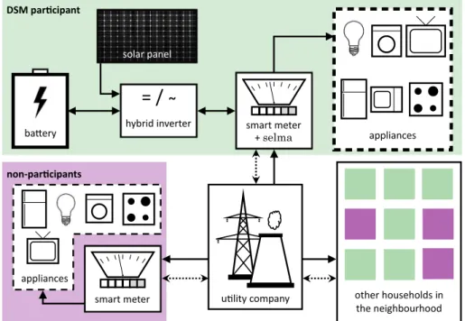
Fig. 1 Systematic sketch of the neighbourhood. Solid arrows stand for power flow, while dotted arrows stand for information flow. The top half of the figure represents a participating household of the DSM scheme. It is equipped with a lithium-ion battery and a solar panel. The solar panel can directly charge the battery, but to run any appliance its direct current needs to be converted to alternating current by the inverter. The smart meter collects data and executes the schedule obtained from the author’s scheduling softwareselma, which is based on a dynamic game. A non-participating household is depicted in the bottom left corner. It is also equipped with a smart meter, collecting data and communicating with the utility company. The complete neighbourhood consists of a number of households (cf. bottom right) that belong to either one of the shown categories. All of them are served by the same utility company
We assume that theMhouses are served by the same UC. In order to incentivise consumers to participate in the DSM scheme, the UC offers them a specific pricing scheme, which eventually reduces their electricity bills. Details can be found in Sect.2.3. Let us denote the set of households who participate in the DSM programme byN ⊂M, whereMis the set of all households in the neighbourhood. The total number of participants isN = |N|. Besides the different pricing scheme, the participants of the DSM possess their own battery storage system and have solar panels installed. An overview of the neighbourhood is shown in Fig.1. The DSM scheme can be seen as a protocol, which is gone through repeatedly. In our study, the protocol is run once per day. Note that this is a completely automated process run by our scheduling softwareselma(short for: Scheduler for Electricity in Local MArkets), which needs to be installed on a consumer access device given to each participant of the scheme. The algorithm to obtain the schedules is based on a discrete time dynamic game, which will be introduced in Sect.3.1.
Before the start of each scheduling period,selmaforecasts the demand1of the respective household for each intervalt∈T of the upcoming day. This information is sent to the UC. The smart meters of non-participants are not able to forecast their own demand. Thus, the
1As of today, the forecasting module is not included intoselma. For this study, we assume this information
UC performs the forecasting step for these households, based on historically collected data. Eventually, forecasted demand curves are aggregated and the information is sent to each DSM participant. Note that no information about individual neighbours is shared, but only aggregated information. This provides anonymity to all consumers.
Based on this input, the households play a dynamic non-cooperative game (cf. Sect.3). The outcome of the game is a set of schedules, one for each household, which specify how they can make best use of their battery system. The households will follow these schedules throughout the day, even if their actual demand differs from the forecasted one. In Sect.4, we investigate the influence of the forecasting error and show the robustness of the approach even in the worst-case scenario. At the end of the scheduling period, the electricity costs for each consumer is calculated based on the agreed pricing terms and the protocol starts over again.
2.2 Individual Households
Households that participate in the DSM scheme are equipped with a lithium-ion battery and PV cells. In this subsection, we introduce the battery model and clarify how the battery can be used. Moreover, details on the PV system are provided. Finally, we clarify the terminology ofdemand,net demand, andloadof a household based on the usage of their battery and PV cells.
2.2.1 Battery Model and Decision Variables
In this paper, we employ the same battery model as used in [17]. This includes charging, discharging, and self-discharging characteristics of a lithium-ion battery. In fact, the same model may also be applied for lead–acid battery systems (but not nickel-based batteries due to their different charging behaviour). As all our simulations are based on a real-world lithium-ion battery system, in the following we will only refer to them as such.
ChargingLithium-ion batteries are charged in a two-stage process [22]. In the first stage, the state of charge (SOC) increases linearly. This stage is called the ‘constant current’ (CC) stage, with a charging rate limited byρ+>0. In the second stage, i.e. the ‘constant voltage’ (CV) stage, the effective charging rate levels off exponentially towards the point where the SOC reaches the nominal maximum capacitysmaxof the battery. The point of transition from
the first stage to the second is indicated by a SOCs∗and an associated timet∗, which needs to be specified for the respective battery. During both stages, we additionally consider losses due to the specific charging efficiencyη+ with 0 ≤ η+ ≤ 1. Additionally, certain losses occur from the hybrid inverter (cf. Fig.1), modelled byηinvwith 0≤ηinv≤1. The hybrid
inverter transforms the direct current from either the battery or PV into alternating current at usable voltage and frequency for the household appliances. It also works in the reverse direction to charge the battery.
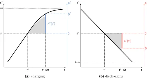
To obtain an insight into how the households can make use of their battery system, let us look at a specific example (cf. Fig.2a). Given a certain value for the SOC, e.g.s, we can associate a timetand thus specify a point on the charging curve.
Within the next interval of lengthΔt, the decision variablea+of how much to charge the battery will lie inH+s=a+|h+s,a+≤0, with
h+s,a+= −a+ a+−φ+s . (1)
(a) (b)
Fig. 2 Schematic illustration of the charging and discharging behaviour of a lithium-ion battery. The graph
on the left (right) shows the characteristic charging (discharging) curve. Given a certain state of charges, the grey area stands for the achievable state of charge within the following interval. The right axes represent the possible decisions when charging (discharging), whereH+s(H−s) summarise the decision intervals. The discrepancy between the achievable state of charge and the decision interval are due to losses, i.e. imperfect efficiencies while charging (discharging)
In other words,a+is limited by 0<a+≤φ+s<smax−s. We use the notation above
to comply with the one shown in [13]. The upper limitφ+sis described by the charging curve, as described above,
φ+s= ρ+t if CC charged smaxγ1exp −γ2t if CV charged , (2)
whereγ1, γ2are defined such that the charging curve is smooth at the transition point(t∗,s∗).
The discrepancy between the grey-shaded area and the charging curve in Fig.2(a) results from an imperfect charging efficiency. In fact, based on the decision variablea+the SOC of the battery changes according to the charging transition equation
st+t=st+ηinvη+a+. (3)
Discharging and Self-DischargingWe model the discharging behaviour of lithium-ion batter-ies by a linear decrease in the SOC. Here, the slope is given by the discharging rateρ−<0. In order to account for the usual sharp drop off of the discharging rate at low capacities, discharging is prohibited below a minimum SOCsmin. Again, we also consider losses due to
the specific discharging efficiencyη−with 0≤η−≤1 and the hybrid inverter.
In Fig.2b, a specific example is given, to clarify how the user can discharge its battery. Within the respective interval, the decision variablea−of how much to discharge the battery will lie inH−s=a−|h−s,a−≤0, with
h−s,a−= a− −a−+φ−s . (4)
In other words,a−is limited bys−smin< φ−
s≤a−<0 and φ−s=ρ−tη
The dependency onsin (5) is implicitly given by the fact that we cannot go lower than smin. Note thatφ− also depends on the efficiency parameter, such that the actual amount
taken from the battery in correspondence with the decision variablea−(grey-shaded area in Fig.2b) is given by the discharging transition equation
st+t=st+ a − ηinvη−.
(6) In the following subsection, we will see thatφ−is additionally limited by the demand of the specific household, i.e. one can only discharge as much as is needed to run all appliances.
Whenever the battery is neither charging nor discharging, it will be subject to self-discharging. We model this type of behaviour with an exponential decline. This case corresponds to the decision variablea=0. The respective self-discharging transition equa-tion is given by
st+t=st·(1+ ¯ρ)t (7)
whereρ <¯ 0 is the self-discharging rate.
For later usage (cf. Sect.3.1), we summarise the transition equations for charging, dis-charging, and self-discharging into a single transition equation f, i.e.
s(t+t)= f(s(t),a)= ⎧ ⎪ ⎨ ⎪ ⎩ s(t)+ηinvη+a, a>0 s(t)+a/(ηinvη−), a<0 s(t)·(1+ ¯ρ)Δt, a=0 . (8)
Furthermore, we combine the restrictions of the decision variable due to the battery restric-tions for charging and discharging, i.e.
h(s,a)= a−φ+(s) −a+φ−(s) . (9) 2.2.2 PV Model
We model the solar panel as an additional source of electricity besides the grid connection. The output of thenth household’s PV system during intervaltis denoted bywtn. It can serve two purposes: (1) direct usage by household appliances and (2) charging the battery. Whereas direct usage is influenced by the efficiency of the hybrid inverter, charging the battery does not require any inversion and thus only depends on the charging efficiency of the battery.
An important parameter of the PV installation is the nominal kilowatt peakkWpof the system. It is a measure of the size of the system and denotes the maximum output that can be expected under standardised conditions. A PV system which operates at its maximum capac-ity, e.g.kWp=3 kW, for one hour will produce 3 kWh. Note that identifying the optimal size of the PV installation does not fall within the scope of this article. An approximated scale is obtained from Zhang and Grijalva [29] and Olaszi and Ladanyi [15] (cf. Sect.4.1).
2.2.3 Demand, Net Demand, and Load
We define the demandd¯mt ≥0 of a householdm ∈Mas the amount of electricity that is needed to run all its appliances during the time intervalt∈T. Thus, the total daily demand schedule can be written asd¯m=
¯
demand cannot be shifted. Thus our approach is fully non-intrusive and does not influence the behaviour of the user.
Combining the demandd¯t
nof a householdn∈N with the generated electricitywtnfrom
the solar panel gives the net demand
dnt = ¯dnt −ηinvwnt , (10)
whereηinvis the efficiency of the inverter (cf. Fig.1). Theoretically, this value can be smaller
than zero, i.e. when the effective generation is larger than the demand in the specific interval. Practically, we ensurednt ≥0 by storing all excess energy directly in the battery. For house-holdsm∈/N, that do not participate in the DSM scheme, the net demand is identical to the demand.
Letlmt denote the load, i.e. the amount of energy drawn from the grid by householdm∈M during intervalt∈T. For households which do not participate in the DSM scheme, the load equals their demand. For the others, the load depends on the decisionatntaken at the specific interval. In other words, it combines the net energy demand with the amount of energy that is charged or discharged by the battery
lnt =dnt +ant , (11)
where max−dt n, φ−
≤at
n ≤φ+. The lower boundary expresses the fact that one cannot
discharge more than is actually needed to fulfil the net demand, while at the same time all battery restrictions remain valid. Due to this condition and (10), we ensure thatlmt ≥0 for allm∈Mand all intervalst∈T. We writelm =
l0m, . . . ,lmT−1for the schedule of loads of a specific household. Furthermore, we can calculate the total load on the grid for interval tby
Lt=
m∈M
lmt . (12)
Similarly, we define the average aggregated load of all households other thannduring time intervaltby Lt−n = 1 M−1 m∈M\n lmt . (13) 2.2.4 Forecasting Errors
The DSM protocol states that households send a forecast of their net demand to the UC. This depends on the demand as well as the electricity generated by the solar panel. Both variables will introduce errors that need to be accounted for. In this paper, we consider the worst-case scenario. [3] gives a comprehensive overview of the current techniques for short-term demand forecasting. They specifically investigate how combining forecasts obtained from an integrated auto-regressive moving average, an artificial neural network, and a similar day approach can improve the short-term load forecast. From [3], we obtain an upper limit for the forecasting errord, expressed as a percentage of the actual demand. Similarly, [5] gives
an insight into 24-hour PV power output prediction. The forecasting errorwis also given as a percentage of the actual generation.
The worst-case scenario is constituted when these two errors carry opposing signs and are correlated between all the participants. This becomes clear from (10), since both contributions for the net demand enter with different signs. Intuitively, it makes sense that in the worst case
the forecasted net demand is smaller than the actual demand. This is because a too small forecasted net demand does disguise the incentive to make use of the battery system. With the same argument, the worst-case solar forecast is higher than the actual one. It might imply a sufficient SOC of the battery, when in reality more charging would have been necessary. 2.3 The Utility Company
Throughout the paper, we assume a single utility company (UC) serves all the consumers in the neighbourhood. The UC runs a DSM scheme in order to reshape the load profile. To be more precise, they want to achieve a flatter profile such that investments into fast ramping technology, which is needed to deliver peak demand, can be reduced. The incentive for the users to limit consumption during peak hours is given by a dynamic pricing tariff: the cost per energy unit is calculated separately for each interval and depends on the aggregated load of all users in the neighbourhood. Following [11,12,17,28], we employ a quadratic cost function gt:
gt(y)=c2·y2+c1·y+c0, t ∈T, (14)
whereyis the aggregated load at timet given byLt and the coefficientsc2 > 0,c1 ≥0,
andc0 ≥0. Similar to [11,17,24], we employ a proportional billing scheme, where each
participant of the DMS scheme pays for their share of the consumption, i.e. the electricity billBnyields Bn = −Ωn t∈T gt ∀n∈N, (15) with Ωn = tlnt t klkt . (16)
For households that do not participate in the DSM scheme, a standard fixed-price tariff is employed, i.e.
Bm= p
t
lmt ∀m∈M\N. (17)
3 Dynamic Battery Scheduling Game
In this section, we formulate the non-cooperative dynamic game between the households that possess individual energy storage and photovoltaic (PV) installations. To do so, we introduce the relevant notation and relate it to their respective ‘real-world’ meaning according to our system (cf. Sect.2). Furthermore, the notion of a Nash equilibrium (NE) is defined and an important result concerning the link between the NE for the whole game and the NE for a subgame is provided. Subsequently, a dynamic programming algorithm is presented from which we derive a closed-form expression of the best response, i.e. the best decision a player can make in response to fixed decisions of other players. Eventually, we use this result to construct an iterative algorithm that computes a NE of the game.
3.1 Definitions and Game Formulation
Formally, the game belongs to the category of discrete time dynamic games (cf. [13]), where players make their decisions sequentially in stages. These stages directly correspond to the daily intervals introduced in Sect.2.1. For each stage, we define a state of the game, i.e. the current state-of-charge (SOC) of all batteries, representing the configuration of the overall system. Furthermore, we define a transition equation that models the evolution of this state based on the decisions of the players. In other words, the players will choose actions that are directly related to their battery usage, which in turn depends on the state of the game. We consider a game with open-loop information structure, which means that the initial state of the game is known by all players. In this game, players want to minimise their energy bill, i.e. their utility function, which depends not only on their own but also on the decisions of all other players. In a nutshell, we have:
Definition 1 Our discrete time dynamic game with open-loop information structure consists of the following components:
(1) A set ofplayers, i.e. participating households (cf. Sect.2.1),N = {1,2, . . . ,n, . . . ,N}, whereN denotes the number of players.
(2) A set ofstages, i.e. intervals (cf. Sect.2.1),T = {0,1, . . . ,t, . . . ,T −1}, whereT denotes the number of stages and thus the number of decisions a player can make in the game.
(3) Scalarstate variables snt ∈ Sn ⊂ Rdenoting the SOC of thenth player’s battery at
staget∈T ∪ {T}. Collectively, we denote the state variables of all players at stagetby st:=s1t,s2t, . . . ,stN∈S :=S1×S2× · · · ×SN ⊂RN. In the open-loop information
structure, it is assumed that theinitial state s0is known2to all playersn∈N.
(4) Scalardecision variables ant ∈ Htnsnt ⊂ An ⊂ R(for definition of Htn see item
(5)) denoting the usage of the battery of thenth player at timet ∈T. Collectively, we denote the decision variables of all players at stagetbyat :=at
1,at2, . . . ,atN
∈A:= A1×A2× · · · ×AN ⊂RN.Furthermore, we define theschedule of battery usageof
an individual playern∈N as a collection of all its decisions in the stages of the game byan :=
an0,an1, . . . ,anT−1. Astrategy profileis denoted bya:=(a1,a2, . . . ,aN).
(5) A set ofadmissible decisionsHn s0 n :=an|htn st n,atn ≤0,t ∈T⊂ RT for the
nth player. The functionhtnsnt,atnhas been defined in (9) Sect.2.2.1, capturing the restrictions posed on the battery. We denoteHtnsnt:=ant |htnsnt,ant≤0⊂R (6) Astate transition equation
stn+1= fntsnt,ant, t∈T, n∈N, (18) governing the state variablesstTt=0. The function fntsnt,antis the discretised version of the transition equation (8) defined in Sect.2.2.1, showing how a decision of the player influences the state of its battery for the upcoming stage.
(7) Astage additive utility function Un sn0, (an,a−n) = −gnT snT − T−1 t=0 gtnsnt,atn,a−tn (19)
2Later, we will see that the solutions/schedules require the players to deplete their battery towards the end
of the scheduling period (cf. finite-horizon effect) to achieve maximum utility. This means as long as none of the players deviates from their respective schedule this knowledge is implicitly shared.
for thenth player, wherea−n:=(a1,a2, . . . ,an−1,an+1, . . . ,aN)denotes the decisions
of all other players. The functiongt n st n, at n,a−tn
has been defined in (14) Sect.2.3 capturing the costs to thenth player at thetth stage. Note that the utility function depends only on the initial state variablesn0, since the subsequent statessntare determined by (18). The function gTn snT =snT (20)
expresses a penalty for thenth player that is incurred by ending up in statesnT, i.e. its SOC, at the end of the scheduling period.
We represent the decision problem of thenth player as the following optimisation problem:
Gn(a−n) given s0∈S maximise an Un sn0, (an,a−n) subject to ant ∈Htnsnt snt+1= fntsnt,atn (21)
Moreover, the game is referred to as{G1,G2, . . . ,GN}. Definition 2 A strategy profile aˆ = aˆ1, . . . ,aˆN
is a Nash equilibrium for the game
{G1, . . . ,GN}if and only if for all playersn∈N we have
Un sn0,aˆn,aˆ−n ≥Un sn0,an,aˆ−n , ∀an ∈Hn sn0. (22)
3.2 Analysis of the Game
In order to analyse the game{G1, . . . ,GN}, we follow the dynamic programming (DP) idea
by Nie et al. [13]. To do so, we introduce notation for subproblems of (21). Furthermore, we show an important result about Nash equilibria for these subproblems, which constitutes the basis for the DP algorithm. Applying the general algorithm eventually leads us to an analytic formulation of thenth player’s best responseaˆn, given the strategiesa−nof other players at
stagetof aT-stage game.
3.2.1 Subgame Formulation
For subproblems that are only interested in decisions taken from stagetonwards, we write: stn,T−1:= stn, . . . ,snT−1 , st,T−1 := st, . . . ,sT−1 ant,T−1:= atn, . . . ,anT−1 , at,T−1:= at, . . . ,aT−1 UnT−t snt, ant,T−1,a−t,nT−1 = −gnT snT − T−1 τ=t gnτsnτ,anτ,a−τn Ht,T−1 n stn :=ant,T−1|hτnsτn,anτ≤0, τ =t,t+1, . . . ,T−1 .
Fort∈T, we define a subproblem of thenth player as the following optimisation problem: GTn−t a−t,nT−1 given st ∈S maximise an UnT−t snt, ant,T−1,a−t,nT−1 subject to atn,T−1∈Htn,T−1 snt snt+1= fnt snt,atn (23)
Therefore, the subgame is referred to as
G1T−t,G2T−t, . . . ,GTN−t
.
Theorem 1 Letaˆ=aˆ0, . . . ,aˆT−1constitute a Nash equilibrium for the game{G1, . . . ,GN}
with the corresponding trajectories of states sˆ = sˆ0, . . . ,sˆT. Consider the sub-game
GT1−t, . . . ,GTN−t
for each t ∈ T. Then, the truncated strategy aˆt,T−1 =
ˆ
at,aˆt+1, . . . ,aˆT−1comprises a Nash equilibrium for the subgame
GT1−t, . . . ,GTN−t
.
Proof The proof can be found in ‘Appendix A.1’.
3.2.2 The DP Algorithm and Derivation of the Best Response Solution
Based on the results of the previous subsection, we can formulate the following DP algorithm to find the solution to the decision problemGn(a−n)(21), i.e. the optimal decision for the
nth player given the decisionsa−n of the other players.
Algorithm 1:DP algorithm for playern∈N to find the solution to (21). Input:T,a−n,s0 t←T 1 for eachsT ∈Sdo Vn0(snT)←gnTsnT 2 whilet>0do t←t−1 3 for eachst ∈Sdo ˆ ant ← argmax at n∈Htn(snt) −gntsnt,ant,a−tn−VnT−t−1ft snt,atn VnT−t(snt)← max at n∈Htn(snt) −gntsnt,ant,a−tn−VnT−t−1ft snt,atn end end end Output:aˆn
Let us apply Algorithm1to obtain the result to the decision problemGn(a−n)(21) in
closed form. Note that both for loops (lines1and3) are treated implicitly by keepingsTand
stunspecified throughout the computations.
Given the total scheduling lengthT, the aggregated decisionsa−nof all other players, and
the initial SOCs0of the batteries, at the first step (t=T) we setVn0(snT)=snT according to (20). With this, we enter the while loop (line2) which overwritestto now representt=T−1. We solve for the best decisionaˆTn−1by solving the following problem:
ˆ anT−1=argmax anT−1 gnT−1 −c2 dnT−1+anT−1+LT−−n1 2 −c1 dnT−1+anT−1+LT−−n1 −c0 −snT−1−anT−1 V0 n
where we made use of the transition equation (18) to rewriteVn0. The solution is computed as
ˆ
anT−1= −snT−1, and subsequently we have
Vn1= −c2 dnT−1−snT−1+LT−−n1 2 −c1 dnT−1−snT−1+LT−−n1 −c0.
With this, the first step is done and we again overwritetto now representt=T−2. In this stage, we solve the following problem:
ˆ anT−2=argmax aTn−2 −gnT−2 snT−2, anT−2,a−Tn−2 +c2 dnT−1− snT−2+anT−2 +LT−−n1 2 +c1 dnT−1− snT−2+anT−2 +LT−−n1 +c0.
The solution is computed as
ˆ anT−2= 1 2 dnT−1−dnT−2−snT−2+L−T−n1−LT−−n2 , from which we obtain
Vn2= −c2 2 dnT−1−dnT−2−snT−2+LT−−n1−LT−−n2 2 −c1 dnT−1−dnT−2−snT−2+L−T−n1−LT−−n2 −2c0,
finalising the second step. This procedure can be done for all subsequent steps. As the equations increase quickly in size, they become infeasible to quote here. Fortunately though, our calculations provided insight into recurring patterns, which all the solutions seem to follow. Eventually, the solution for an arbitrary stagetof theT-stage dynamic game can be written as
ˆ atn= 1 T −t T−1 τ=t+1 dnτ+Lτ−n−snt −(T−t−1)dnt +Lt−n (24)
Note that during the derivation the nonlinear battery constraints are not strictly considered. Similar to the forecasting errors (cf. Sect.3.3), these are considered in our simulation when the equilibrium schedules are actually executed. Furthermore, we want to highlight that the optimal decision (24) fornth player at timetonly depends on the current and future forecasted net demand data, the current SOC of the battery, and the average load (13) on the grid caused by all the other households. This can be vaguely reminiscent of an alternative and elegant mean-field-type approach [6,8] in which each player reacts directly to an aggregated signal from the group.
3.3 The Algorithm and Execution of NE Schedules
Similar to [17], we make use of a best response algorithm (cf. Algorithm2) to find the solution to the game. Whereas in [17] an extensive search for optimal schedulesaˆnwas performed,
Algorithm 2:Best response algorithm for finding a pure NE based on [23] Input:T,s0
initialise random strategy profilea=(an,a−n)
1 whilethere exists a player n for whom anis not a best response to a−n do 2 for eachn∈N do
3 for eacht∈T do ˆ
ant ←best response toa−nbased on (24)
end an ← ˆ an0, . . . ,aˆnT−1 end end Output:aˆ
here we can compute the best response for each stage (line3) analytically by means of (24) and concatenate the results to obtain the optimal scheduleaˆnin response toa−n. Performing
this computation for each playern∈N(line2) results in a new strategy profilea. We iterate this (line1) as long as ‘there exists a playernfor whomanis not a best response toa−n’. In
the actual implementation, this check is done by comparing the current strategy profile with the one obtained from the previous iteration. If it did not change, up to machine precision, an equilibrium is reached andaˆ=aˆn,aˆ−n
constitutes the Nash equilibrium. This iterative approach is a type of cobweb method [2] which theoretically does not converge for every given scenario. An analysis of the convergence behaviour is performed in Sect.4.2.
Based on the definition of a NE, no household can benefit from unilaterally deviating from its respective schedule. Nonetheless, we have to keep in mind that it is based on forecasted demand and renewable generation. Whenever either the demand or the generation does not match the forecasted value, it might not be possible anymore to strictly follow this NE
schedule. In the analysis in the subsequent sections, we assume that every individual always seeks to be as close as possible to their determined NE schedule. To illustrate the idea: imagine a NE schedule of householdnrequires them to discharge an amountx in a certain interval. Due to a forecasting error for the renewable generation, this has not been charged fully and can thus not be delivered. In this case, the schedule will discharge as much as possible during this interval. The deviation from the NE will decrease the benefit in terms of PAR reductions and achieved savings for the consumer. Anticipating the results, we want to highlight that in the following section we show that the solution is robust with respect to these deviations and gives considerable improvements in comparison with other approaches in the literature.
4 Results and Discussion
In this section, we firstly summarise important simulation parameters and introduce the spe-cific data sets for electricity demand and generation from the photovoltaic (PV) installation. After analysing the convergence behaviour of the iteration algorithm, we compare the game-theoretic approach introduced in this manuscript (cf. Sect.3.1) with a simpler non-cooperative static game, revealing the advantages of the dynamic treatment. Subsequently, the analysis of how the participation rate of the DSM scheme and the forecasting errors influence the scheduling outcome is shown. Finally, we consider the influence of the composition of the neighbourhood on the peak-to-average ratio (PAR) reduction. This is an important mea-surement of the effectiveness of the DSM scheme. We consider the PAR of the aggregated electricity load (12) over the respective scheduling period. It is defined by
PAR=T·maxt∈T L
t
t∈T Lt
. (25)
4.1 The Simulation Setup
In the real-world application, the smart meter of individual households collects data about electricity demand and generation from the available PV installation. As specified in Sect.2.1, the demand-side management (DSM) protocol requires participants to send forecasts of the demand and generation to the utility company. These forecasts are based on historically collected data. In order to run our simulations, we omit this forecasting step and rather make use of two publicly available data sets.
Demand dataThe demand data stem from the OpenEI data set [27]. It contains 365 days of simulated hourly data3for households in TMY3-locations in the USA [14]. The building models used for this simulation can be found in [26]. Based on an additional survey, all buildings are put into one of three different categories. They differ with respect to their overall consumption. Following [27], we refer to them as LOW, BASE, and HIGH consumers. For all simulation runs, we picked the sameM=25 households, in close vicinity to each other, to represent our neighbourhood. With respect to their consumption categories, we have seven LOW, nine BASE, and nine HIGH users.
PV dataData for the PV generation are based on real-world measurements [19] in the UK. They contain hourly values for days between September 2013 and October 2014. Note that latitude and climate zone of the measurement location are similar to the ones of the demand data. Under the assumption that the weather for all households in the neighbourhood is the
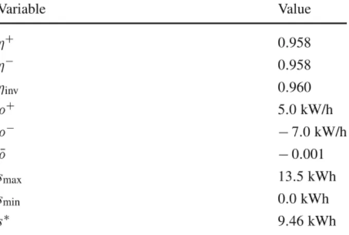
Table 1 Battery parameters Variable Value η+ 0.958 η− 0.958 ηinv 0.960 ρ+ 5.0 kW/h ρ− −7.0 kW/h ¯ ρ −0.001 smax 13.5 kWh smin 0.0 kWh s∗ 9.46 kWh
Parameters for a Tesla-inspired [25] home battery storage system
same, we use data from the same site for each of them. An estimate for thekWpvalue is obtained from looking at the highest hourly output in the course of a whole year. Its value is wmax=3.7 kWh, which is why we assumekWp≈4 kW. We account for different sizes of
PV installations by scaling the data set with a household specific factorpn. About 6% of the
collected data were corrupted. We set all these values tow=0.0 kWh. This does not pose any problem for our simulation results, but can be seen as realistic failures of the installation. Battery and pricing parametersThe parameters of the battery are based on the Tesla Power-wall 2 [25] data sheet. The choice to employ this battery system is motivated by two reasons: (1) the same battery was used in [17], allowing for a direct comparison of the results; (2) a non-extensive analysis of different battery systems showed that the Tesla Powerwall 2 qual-ifies as a representative of state-of-the-art technology. Please see ‘Appendix A.2’ for more details. A summary of the battery parameters is given in Table1. The data sheet only specifies the round-trip efficiencyη=η+·η−of the battery. Without loss of generality, we assume that charging and discharging contribute equally, yieldingη+=η−=√0.918.
For the parameters in the cost function (14), we use c2 = 0.03125 $/MW2, c1 =
1.0 $/MW, andc0 = 0, following other studies [17,20]. This allows to directly compare
our results. In ‘Appendix A.3’, the influence of these coefficients on the potential savings for the households is analysed.
4.2 Convergence Behaviour of the Algorithm
Let us provide an insight into the convergence behaviour of Algorithm2. The condition that needs to be fulfilled to declare equilibrium is stated as ‘there exists no playern for whom his current actionan is not a best response to the actionsa−n of the other players’
(cf. Algorithm2, line1). Within our specific implementation ofselma, the stopping criteria are based on the L2 difference between the action profiles of two consecutive iterations, i.e. when this difference is smaller or equal to 10−15the algorithm breaks out of the loop.
Associated with the current action profile during each iteration are also the energy bills for each participant.
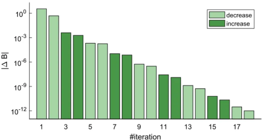
Fig. 3 Convergence analysis of Algorithm2. The change in the average bill of the DSM participants between consecutive iterations is plotted over the iteration number. The ordinate is scaled logarithmically. Bars are coloured according to the algebraic sign of the change. The specific data points stem from a simulation in Sect.4.4with 64% participation rate and without forecasting errors (Color figure online)
0 20 40 60 80 100 N/M (%) 0 5 10 15 20 25
average number of iterations
Fig. 4 Iteration statistics. The mean number of iterations per day is plotted over the participation rate in per
cent. The values stem from the simulations undertaken in Sect.4.4. In addition to the average over 365 days, the standard deviation is shown for each data point.
ResultsIn Fig.3, the absolute change in the average billB=1/N
nBn(cf. (15)) is shown
for a randomly selected day of the simulation shown in Sect.4.4. To cover the large scale of different changes, a logarithmic representation is chosen. The respective sign of the change is then expressed in the colour of the bar.
Figure4shows how the number of average iterations per day depends on the number of participants in the DSM scheme. The values are again taken from the simulations in Sect.4.4. DiscussionThe results give evidence of a correctly working iteration algorithm (cf. Algo-rithm2). From Fig. 3, we see that between any two consecutive iterations, the absolute change in the average electricity bill is monotonically decreasing. Furthermore, we observe that the rate of this decrease is almost linear in the semi-logarithmic plot, hinting towards an exponential relationship.
Due to the exponential convergence towards a Nash equilibrium, only few iterations are needed to obtain the equilibrium schedules. The specific number of iterations depends on the number of participants taking part in the DSM scheme. This is comparable to the ones shown in [12]. Figure4shows that the average number of iterations increases monotonically with the number of participants. Moreover, the variation across the number of iterations for individual scheduling periods is small, as shown by the standard deviation. This is a strong result, as it shows that the convergence properties are insensitive to different demand data of the individual participants. During experimentations with the code, more than one million games were solved which all converged to a Nash equilibrium.
The small number of iterations directly translates to small computational times and thus does not hinder a real-world application. Typical 365-day simulation runs take about 30 s on a single core of ani7-3770SCPU and require less than 1 GB of memory. Note that in the real-life scenario, the scheduling process is initiated once before the scheduling period and only needs to calculate the equilibrium schedules for the upcoming day. In summary, we expect no difficulties in implementing a DSM scheme based on our scheduling softwareselma.
4.3 Comparison Between a Static and a Dynamic DSM Scheme
In [17], a similar DSM scheme to the one described in Sect.2.1was examined. Both are based on a battery scheduling game for households of a neighbourhood served by the same utility company (UC). Their main difference is the underlying game that determines the schedules for the upcoming day. Whereas in this paper we employ a discrete time dynamic game, Pilz and Al-Fagih [17] made use of a simpler non-cooperative static game in which players were only able to choose between four discrete options for each interval. For a more thorough description please see [17]. For the sake of comparison, none of the households is equipped with PV cells.
In this subsection, we compare the two approaches with respect to their success in reducing the PAR of the aggregated load. To this end, the same parameters for each household and also the same demand data are used. Households do not have the capability of on-site generation, but are equipped with the same batteries (cf. Table1). The upcoming day is divided into T =12 intervals, and we assumeN =M=25, i.e. every household takes part in the DSM scheme. As in [17], we simulate full weeks by using the state-of-charge (SOC) values of the batteries at the end of the scheduling period as the initial configuration for the following one. ResultsFigures5a, b show the aggregated load curves achieved by the DSM schemes for forecasts given by week 12 and week 38 of the demand data set [27], respectively. For completion, we also simulated week 25 and week 51 as done in [17]. A summary of the achieved results is given in Table2.
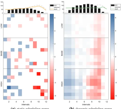
On average, a 14% and 32% decrease in the PAR value was achieved by the static and the dynamic games, respectively. To understand the differences of the outcomes, we explicitly look at the schedules that are obtained in the NE of the respective games. Figure6shows these schedules exemplarily for day 5 of week 38 (Fig.5b, cf. Figure 3 in [17]) together with the aggregated load and aggregated SOC above it. Each row illustrates the equilibrium schedule of one household.
DiscussionComparing the aggregated load curves (cf. Fig.5) shows that a DSM scheme based on a dynamic game can achieve an almost flat profile. Nevertheless, depending on the given data, the outcome of the scheduling is subject to a finite-horizon effect. Empirically, we observe peaks and troughs at the end of the scheduling period if the demand for the final
day 1 day 2 day 3 day 4 day 5 day 6 day 7 time 0 20 40 60 80 100 120 aggregated load (kWh) reference static game dynamic game (a) week 12
day 1 day 2 day 3 day 4 day 5 day 6 day 7 time 0 20 40 60 80 100 120 aggregated load (kWh) reference static game dynamic game (b) week 38
Fig. 5 Load comparison. The aggregated load of all households in the neighbourhood is plotted over time.
The simulation domains cover seven days that were each scheduled consecutively. The aggregated demand is given as a reference. The orange curve results from a DSM scheme employing a static scheduling game [17], while the green one stems from a DSM scheme employing a dynamic game. Other than the underlying game structure, all parameters are identical (Color figure online)
interval is lower than the average demand of the whole day. This indicates that the starting time of the DSM scheme has an influence on the achievable outcome. Nonetheless, this parameter is fixed through the DSM scheme protocol, thus asking for alternative solutions to the finite-horizon effect. Future work will aim to eliminate the influence of the starting time altogether.
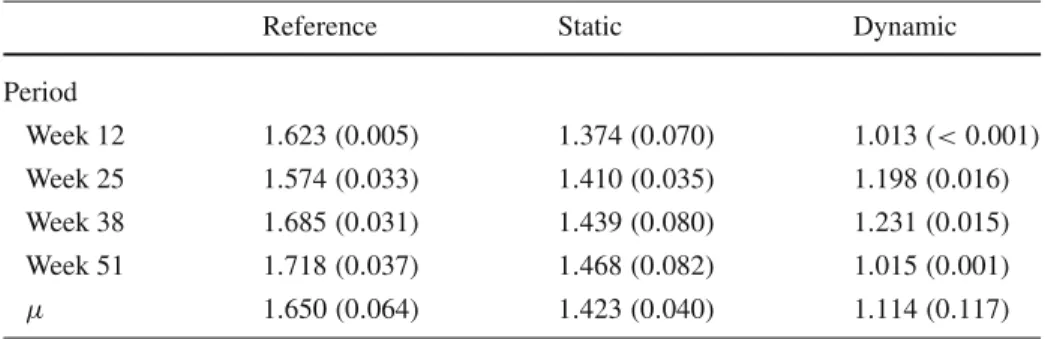
In Table2, we observe that on average the dynamic game reduces the PAR value more than twice as much as the static game. However, with respect to the individual weeks the static game shows a smaller standard deviation of 0.04 and thus seems to be more consistent. Its achieved reductions are all between 10.4 and 15.3%, while the range of reductions by the DMS scheme with the dynamic game is 23.9–40.9%. The differences with respect to the standard deviations is again owed to the finite-horizon effect. It is also present in the case with the static game, but, due to generally worse outcome, does not alter it as much as the results of the dynamic scheduling game.
We can further understand the differences between the static and dynamic game from Fig.6. The restriction to four discrete options for each interval in the static case, i.e. (1) remain idle, (2) charge half interval, (3) charge full interval, and (4) use battery, results in a
Table 2 PAR comparison
Reference Static Dynamic
Period Week 12 1.623(0.005) 1.374(0.070) 1.013(<0.001) Week 25 1.574(0.033) 1.410(0.035) 1.198(0.016) Week 38 1.685(0.031) 1.439(0.080) 1.231(0.015) Week 51 1.718(0.037) 1.468(0.082) 1.015(0.001) μ 1.650(0.064) 1.423(0.040) 1.114(0.117) Peak-to-average ratios calculated as the average over the individual days of week 12, week 25, week 38, and week 51 for the case without storage system (Reference) and both underlying games of the DSM scheme.μgives the average over all 4 weeks. Static: game employed in [17]; dynamic: game described in Sect.3.1. The values in parentheses represent the standard deviation
majority of intervals where the battery remains idle. This is because of a lack of incentive to charge the battery by the two given amounts. In the dynamic game, players can choose to charge their battery from a continuous spectrum of decisions in a given interval. This difference becomes most apparent when looking at the aggregated SOC of all participants. Whereas the maximal SOC in the static case is approximately 64 kWh, almost twice as much (120 kWh) is charged in the dynamic case. In summary, it shows that the increased flexibility of the dynamic game is better suited to minimise the PAR of the aggregated load.
Note that all these comparisons allow for strong conclusions as they are based on the identical data set [27] and also all the other parameters, such as number of players N and number of time intervalsT, are chosen to be the same. Nevertheless, comparisons with other results in the literature are possible: compared to the work by Nguyen et al. [12], a better PAR reduction is achieved while also the number of iterations to obtain the equilibrium solution is lower by two orders of magnitude. Similarly, the PAR reduction of Yaagoubi et al. [28] is worse than the approach shown in this manuscript. As they schedule not only the battery but also shift other household appliances, a comparison of the computational costs is not appropriate.
4.4 Influence of Participation Rate and Forecasting Errors
The question of how many participants are needed to obtain considerable gains in terms of PAR reduction and savings is important. Moreover, within this subsection the robustness with respect to the forecasting errors (cf. Sect.2.2.4) is shown. To do so, we assume the forecasting error for the demand to bed = 8% for every household [3], which could be
obtained from a forecast performed by an artificial neural network, and is approximately 2.5 times higher than the best forecast obtained by them. This is independent of whether the household participates in the DSM scheme or not. The forecasting error for the solar generation is set tow = 10% in accordance with [5,21]. Rana et al. [21] make use of a neural network and clustering of weather data to forecast half hourly solar power output for the upcoming day. Note that only participants of the DSM scheme are equipped with PV cells and thus subject to the forecasting error. The values are taken to represent a worst-case
Fig. 6 Nash equilibrium schedule comparison. The schedules for all participating households of the demand-side management scheme for a single scheduling period (week 38, day 5, cf. [17]) are shown together with their respective aggregated load and aggregated state of charge (SOC). (a) The underlying game structure is a static non-cooperative game from Pilz and Al-Fagih [17]. Within each interval, players can choose between four discrete decisions. (b) Here, the game structure is the dynamic game introduced in Sect.3.1. Note that the schedules employ the same scaling
scenario. Subsequently, any real-world scheduling result should fall in the interval between the worst-case outcome and the respective outcome without any forecasting error.
We simulate a full year and average over the obtained PAR values for the individual days. All participants are equipped with a lithium-ion battery (cf. Table1) and a solar cell. The size of the PV installation depends on the user’s category. For LOW, BASE, and HIGH consumers, we use pn =0.3,pn = 0.5, and pn = 0.7, respectively. Starting with all 25 households
taking part in the DSM scheme, we eliminated three users, i.e. one randomly selected from each consumer category, in each subsequent run. Non-participant still exhibit the specified forecasting error for their demand.
ResultsFigure7shows the reduction in the PAR value over the rate of participating consumers for the scenarios with and without forecasting errors. It includes not only the mean values, but also the standard deviation. Note that we slightly shifted the results for both runs along the abscissa to increase readability. An additional axis on the left indicates the absolute PAR values. Whereas the PAR reduction is the interest of the UC, the financial rewards, i.e. savings
0 20 40 60 80 100 N/M (%) -40 -35 -30 -25 -20 -15 -10 -5 0 5 PAR reduction (%) 1 1.1 1.2 1.3 1.4 1.5 1.6 1.7 PAR with error without error
Fig. 7 Peak-to-average ratio (PAR) reduction dependency on the participation rate. The mean PAR reduction
in per cent is plotted over the participation rate in per cent. The right-hand axis shows the absolute values of the PAR. In addition to the average over 365 days, the standard deviation is shown for each data point. The simulations were run for a scenario with forecasting errors and one without forecasting errors. Note that the data points are slightly shifted along the abscissa to increase readability
0 20 40 60 80 100 N/M (%) -10 -8 -6 -4 -2 0 bill reduction (%) -8 -6 -4 -2 0 2
difference between values (%)
with error without error difference
Fig. 8 Savings dependency on the participation rate. The mean bill reduction in per cent for participants of the
demand-side management scheme is plotted over the participation rate in per cent. In addition to the average over 365 days and participants, the standard deviation between different participants is shown for each data point. The simulations were run for a scenario with forecasting errors and one without forecasting errors. The difference between the two curves is plotted against the right-hand axis
off the energy bill, are the interests of the participants of the DSM scheme. Figure8shows the average saving per day for all participants both with and without forecasting error. For further insight, it also illustrates the difference between the two curves.
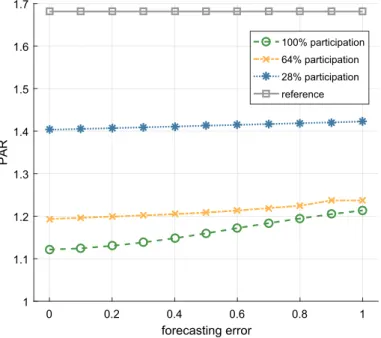
0 0.2 0.4 0.6 0.8 1 forecasting error 1 1.1 1.2 1.3 1.4 1.5 1.6 1.7 PAR 100% participation 64% participation 28% participation reference
Fig. 9 Influence of forecasting error on the achieved PAR value. The PAR values for three different participation
rates are plotted over the forecasting error. Here, the abscissa refers to the worst-case scenario as described in Sect.4.4, e.g. at 0.6 a forecasting error with the magnitude of 60% of the worst-case is assumed. In the reference case, no game is played, so the forecasting error does not influence the PAR value
DiscussionAlthough a worst-case scenario is simulated, the outcome with respect to PAR reduction (cf. Fig.7) and electricity bill (cf. Fig.8) reduction shows considerable gains for the UC and the participants of the DSM scheme.
Without forecasting error, the PAR reduction monotonically improves with the proportion of the participants. This stands in contrast to the results shown in [24], where a minimum is reached at medium range participation rate. In comparison with other studies, such as [9, 12], we conclude that our dynamic game performs as good as their respective scheduling approach. At 100% participation rate, a reduction of−33.3% (5.8%) is achieved, in agreement with the results shown in Sect. 4.3. It should be noted that a perfectly flat load profile corresponds to an approximately−40% reduction of the PAR. Thus, the outcome is close to the theoretical optimum. When looking at the standard deviation, we observe that it is lowest for the simulation run with 52% participation rate and increases towards both ends of the spectrum. On the lower end of participation rate, the fluctuations of the PAR value for different days are just an artefact of the data set in use. Small numbers of participants have not enough influence on the overall neighbourhood to change this. When regarding large participation rates, the PAR value is considerably reduced. The increase in the standard variation for these runs stems directly from the finite-horizon effect already discussed in Sect.4.3.
The results for runs with forecasting errors follow the results without errors closely. Figure9shows how the forecasting error affects the achieved PAR values for three selected participation rates when transitioning from the perfect forecast to the worst-case scenario as depicted in Fig.7. For low participation rates, the difference is negligible but starts to increase when more households participate in the DSM scheme. Nevertheless, even in the worst-case
scenario, a reduction of−27.8% (8.9%) is achieved at 100% participation rate (cf. Fig.7). With respect to the standard deviation, we again recognise similarities to the runs without forecasting errors. Smallest variations in the PAR reduction are obtained for participation rates around 50%, while we again see increasing variations at high participation rates. Here, the increase is distinctly larger than in the other runs. The reason behind this difference is directly explained by the forecasting error. As more participants join the DSM scheme, the absolute amount of deviation from the actual demand and production is increasing.
It is worth noting that the result for a participation rate of 76%, i.e. a reduction of−27.7% (4.4%) (cf. Fig.7), is very promising from a practical point of view. The UC might not be able to convince everybody to participate in the DSM scheme, but can still gain reductions in the PAR value close to what is achievable at maximum participation.
In [18], it is investigated what happens when no forecast is calculated. Rather than calculat-ing the forecast, the demand data of the current day are used as the input to the dynamic game that determines the schedules for the next day. It turns out that this approach is oversimplified and results in distinctly worse outcomes (cf. [18, Figure 5]), i.e. it shows the importance of a suitable forecasting mechanism.
The savings that participants of the DSM scheme can gain increase monotonically with the share of participants. Furthermore, we observe that the variations between different par-ticipants are negligible. This is due to the particular proportional billing scheme employed in the scheme (cf. Sect.2.3). It ensures fairness in the sense that LOW and HIGH consumers can gain equally by signing up for the DSM scheme. The difference between runs with and without forecasting errors reveals that the forecasting error does not influence the bill reduc-tion to a great extent. Since the two curves are almost non-separable to the unaided eye, the difference is shown in the same plot (cf. Fig.8). It becomes clear that the difference is actually decreasing for larger numbers of participants.
This highlights that the dynamic scheduling game ensures robust and beneficial results for the participants of the DSM scheme, even in the worst-case scenario.
4.5 Consumer-Type Dependency
ResultsThe results in Sects.4.3and4.4are all based on a neighbourhood consisting of a mix of the three different consumer types (LOW, BASE, and HIGH). Figure10shows the possible PAR reductions for mono-type neighbourhoods. To allow for comparison,M =25 is kept constant. Furthermore, we use the same forecasting errors ofd =8% andw =10% for
the demand and renewable energy generation, respectively (cf. Sect.4.4). All the simulations consider a scheduling period of a full year.
We also calculated the average savings that are achieved by the participants of the DSM scheme. These results are presented in Fig.11together with the reference of a mixed neigh-bourhood (cf. Fig.8) with forecasting errors.
DiscussionWhen comparing different compositions of neighbourhoods, we can gain further insight into the conditions for which the DSM scheme works most efficiently. At first glance, Fig.10reveals that given a low rate of participants in the scheme, the actual type of consumer is not crucial. Figure 12 shows the difference between the respective results for mono-type neighbourhoods and a mixed neighbourhood. A closer look shows that mono-LOW communities are always worse in reducing the PAR value of the aggregated load than any of the other ones. The results in terms of both the mean PAR reduction and the standard deviation get even worse with more than two-thirds of households participating in the scheme. Similar observations for mono-type neighbourhoods are found in [24].
0 20 40 60 80 100 N/M (%) -40 -35 -30 -25 -20 -15 -10 -5 0 5
PAR reduction (%) HIGH BASE LOW mixed
Fig. 10 Peak-to-average ratio (PAR) reduction for different neighbourhoods. The mean PAR reduction in per
cent is plotted over the participation rate in per cent for different mono-type consumer neighbourhoods. In addition to the average over 365 days, the standard deviation is shown for each data point. For comparison, the results of a mixed neighbourhood (cf. Fig.7) are also presented. Note that the data points are slightly shifted along the abscissa to increase readability
0 20 40 60 80 100 N/M (%) -10 -8 -6 -4 -2 0 bill reduction (%) HIGH BASE LOW mixed
Fig. 11 Savings for different neighbourhoods. The mean bill reduction in per cent for participants of the
demand-side management scheme is plotted over the participation rate in per cent for different mono-type consumer neighbourhoods. In addition to the average over 365 days and participants, the standard deviation between different participants is shown for each data point. For comparison, the results of a mixed neighbour-hood (cf. Fig.8) are also presented
For both mono-BASE and mono-HIGH neighbourhoods, it can be observed that they perform better (<1%) in an interval of medium participation rate than the mixed neighbour-hood. Nevertheless, at N = Mthe obtained PAR reduction is smaller by 1.8% and 4.5%, respectively. Considering the variation of these mean PAR reduction values, it becomes clear that it is most beneficial to have a mixed-consumer neighbourhood.