NCIS: a network-assisted co-clustering algorithm to discover cancer subtypes based on gene expression

c

NCIS: A NETWORK-ASSISTED CO-CLUSTERING ALGORITHM TO

DISCOVER CANCER SUBTYPES BASED ON GENE EXPRESSION

BY

YIYI LIU

THESIS

Submitted in partial fulfillment of the requirements

for the degree of Master of Science in Bioengineering

in the Graduate College of the

University of Illinois at Urbana-Champaign, 2013

Urbana, Illinois

Adviser:

Abstract

Cancer subtype information is critically important for designing more effective treatments. In this thesis, we introduce a new co-clustering algorithm for cancer subtype identification, which combines the information of gene networks to simultaneously group samples and genes into biologically meaningful clusters. We call our method network-assisted co-clustering for the identification of cancer subtypes (NCIS). Prior to clustering, we assign weights to genes: those that play key roles in the network and/or show significant variations among samples would be prioritized. This new approach allows us to rely more on genes that are informative and representative by including the weights as an importance indicator in the clustering step. Here we introduce a new weighted co-clustering method based on semi-nonnegative matrix tri-factorization. We evaluated the effectiveness of the algorithm on large-scale Glioblastoma multiforme (GBM) and breast cancer (BRCA) datasets from TCGA and on simulated datasets. We found that our NCIS method can achieve more reliable results with respect to the clinical features compared to conventional semi-nonnegative matrix tri-factorization methods and consensus clustering. We also train two classifiers for GBM and BRCA subtypes identification based on NCIS’s results.

This new method will be very useful to comprehensively detect subtypes that are oth-erwise obscured by cancer heterogeneity, from various types of cancers based on high-throughput and high-dimensional gene expression data.

Acknowledgments

Many thanks to my advisor, Prof. Jian Ma, for his great help and guidance. I benefit a lot from his insightful ideas on this research work and from his advice on how to perform scientific study. Thanks to my collaborators Quanquan Gu, Jack P. Hou and Prof. Jianwei Han. Quanquan and Prof. Han gave me many suggestions on machine learning methods. Jack provided the gene network he collected for me to use in this work. Thanks to Yang Li and Yang Zhang, who gave me much help in using different tools and leveraging biol-ogy knowledge. Also thanks to all the other members of Prof. Ma’s lab for their helpful discussions.

Table of Contents

2.2 Assigning Weights to Genes . . . 6

2.3 Weighted Co-clustering . . . 8 2.3.1 Objective . . . 9 2.3.2 Optimization . . . 10 2.3.3 Proof of convergence . . . 12 2.3.4 m andcselection. . . 14 Chapter 3 Results . . . 15

3.1 Breast Cancer Dataset . . . 15

3.2 Glioblastoma Dataset . . . 21

3.3 Simulated Datasets . . . 26

Chapter 4 Conclusion . . . 29

List of Tables

1 Main notations . . . 9

2 Cophenetic coefficients for BRCA data . . . 16

3 P-value of the dependence test for different clinical features and BRCA subtypes . . . 17

4 Pathways enriched by BRCA 35 genes . . . 20

5 Pathways enriched by PAM50 50 genes . . . 22

6 Cophenetic coefficients for GBM data . . . 22

7 P-value of the dependence test for different clinical features and GBM subtypes . . . 24

8 Pathways enriched by GBM 30 genes . . . 26

List of Figures

1 Schematic diagram of NCIS . . . 5

2 Heatmap of breast cancer expression data . . . 16

3 Accuracies of BRCA subtype classifiers trained with different numbers of genes 19

4 Expression patterns of ABCC8 subnetwork in BRCA subtypes . . . 21

5 Heatmap of GBM expression data . . . 23

6 Kaplan-Meier survival curves of GBM data . . . 25

7 Accuracies of GBM subtype classifiers trained with different numbers of genes 26

Chapter 1

Introduction

Cancer is a complex disease. All cancers share a common pathogenesis, which is the outcome of a process of Darwinian evolution occurring among cell populations within the microenvi-ronments provided by certain tissues. The evolutionary process can promote cells carrying advantageous genomic alterations that confer the capability to proliferate and survive more effectively, which may consequently invade tissues to cause cancer and eventually metas-tasize. However, for different types of cancers, genomes of somatic cells undergo dramatic but distinct changes during cancer development and progression (Campbell et al., 2010;

Pleasance et al.,2010a,b). Even for the same type of cancer, there are subtypes that harbor unique sets of changes and exhibit different patterns of gene expression (Perou et al.,2000;

Sorlie et al.,2001;Alizadeh et al.,2000;Bhattacharjee et al.,2001;Golub et al.,1999). The subtype information is critically important for designing more effective treatments. Recent advances in next-generation sequencing (NGS) technologies have provided us with an un-precedented opportunity to study the molecular signatures of human cancers in a much more refined manner. Several recent large-scale cancer genomic studies have revealed that the genetic diversity of the same type of cancer (even for the relatively well-characterized breast cancer (Curtis et al., 2012; Stephens et al., 2012; Banerji et al.,2012; Shah et al.,

2012)) is much greater than previously thought. Therefore, better methods are urgently needed to discover cancer subtypes based on high-throughput and high-dimensional data.

In the past decade, many clustering-based approaches have been developed to identify cancer subtypes based on gene expression profiles (Barillot et al.,2012). Typically, expres-sion levels ofd genes measured on nsamples are presented as ad×n real-valued matrix, with rows representing the d genes, columns representing the n samples, and entries for the corresponding expression level. Then a clustering method is applied to partition the columns/rows of this matrix into different clusters such that items within one cluster have more similar expression patterns. The partition of columns offers clues to potential cancer

subtypes while the partition of rows highlights possible co-expressed genes and pathways that might be relevant to each subtype. In this work, we mainly focus on the clustering method for subtype identification. We assume the expression matrix has been pre-processed such that the batch effects and other technical artifacts are already removed.

The most popular clustering methods used in cancer subtype identification include hier-archical clustering (Shai et al.,2003;Network, 2012;Bullinger et al., 2004;Phillips et al.,

2006) andk-means (Phillips et al.,2006;Tothill et al.,2008;Lehmann et al.,2011). These two methods have very intuitive meanings and can capture the nature of the data in many cases. However, in most of the previous works, biological information (such as gene-gene in-teractions) was often not incorporated in the clustering step. Sometimes the clustering result could be very sensitive to measurement error, consequently making subsequent analysis dif-ficult to perform. On the other hand, gene expression profiles generated by high-throughput technologies are often of very high dimension, i.e. the number of genes is far larger than the number of samples, so an appropriate feature (gene) selection method is of vital importance to successful cancer subtype detection. Utilizing prior knowledge of molecular interactions could help elucidate more representative genes. For example, upstream genes that regulate many downstream targets generally have bigger impacts on the overall expression patterns since their changes can lead to changes of these targets.

Indeed, network is important in understanding cancer (Barabasi et al., 2011; Chuang et al.,2007). The interactions between genes will allow us to preform clustering by relying more on modeling the perturbation of a group of related genes rather than individual genes. Therefore, our goal in this work is to develop a method that effectively incorporates network information into the clustering process. To this end, a previous work employed information of biological networks to develop a clustering method (Hanisch et al., 2002). The authors first defined a network distance based on proximity of two genes in the network and an expression distance based on expression level similarity of two genes, and then constructed the overall distance metric as a function of network and expression distance metrics for hierarchical clustering. There was another work that incorporates network into the cluster-ing framework proposed to co-cluster genotypes and phenotypes based on phenotype-gene association matrix (Hwang et al.,2012). The authors did so by adding penalty and regular-ization terms into co-clustering objective to keep the final clustering results consistent with clusters obtained from prior knowledge on disease phenotype similarity network and gene

interaction network. However, similar approaches could be improper for our purpose. First, network distances (as in (Hanisch et al.,2002)) or network-derived clusters (as in (Hwang et al., 2012)) are difficult to define for the patients since there is not a network structure linking all the patients. Second, the rationale that genes are related according to their proximity in the network may not always be helpful for clustering gene expression profiles as neighboring genes can have entirely opposite expression patterns: For instance, if Gene

Adown-regulates GeneB, their expression levels tend to be anti-correlated, so according to the commonly used distance metric for heatmap (1-correlation, Euclidian distance, etc.),A

andB will be clustered into two groups, while their positions in the network is very close. In this work, we integrate network information with expression variation across sam-ples to train a weight for each gene which is then used as an importance indicator in the clustering. Such weights will assist us to select genes with greater priority based on the given dataset and prior knowledge of molecular interactions. The key idea is that genes regulating many other genes and/or showing highly variable expression patterns should be considered as more informative in the clustering process. Another important contribution of this work is that we embed the weights into a “co-clustering” objective function. Un-like traditional one-sided clustering, co-clustering simultaneously clusters both samples and features (Tanay et al.,2005). In co-clustering, similarity is a measure of the coherence of features and samples in bi-cluster (each small block), rather than a function of feature pairs or sample pairs; consequently, it considers about local context and is able to automatically select subsets sharing similar attributes (Cheng and Church, 2000). Previous works have proposed co-clustering methods that are useful in gene expression analysis (Cheng and Church,2000;Cho et al.,2004;Ihmels et al.,2002; Ben-Dor et al.,2003;Murali and Kasif,

2003;An et al.,2012;Eren et al.,2012;Li et al.,2009b;Prelic et al.,2006;Hochreiter et al.,

2010; Huttenhower et al., 2009; Gu and Liu, 2008; Lazzeroni and Owen, 2002; Bergmann et al., 2003). An overview of more co-clustering methods can be found in (Tanay et al.,

2005; Eren et al., 2012; Prelic et al., 2006; Madeira and Oliveira, 2004). The method we use here is based on Semi-Nonnegative Matrix Tri-Factorization (SNMTF) (Ding et al.,

2006; Gu and Zhou, 2009), which is a member of the matrix factorization based cluster-ing family. A common underlycluster-ing motivation of this family of co-clustercluster-ing methods is that there exist some cluster centroids that can characterize the behaviors and trends of their cluster members, so the goal is to minimize the overall distances to cluster centroids,

which mathematically is formed into matrix tri-factorization. Matrix factorization has sim-ple formalization, as compared to other methods, and was shown to be very useful in gene expression analysis (Barillot et al.,2012;Kim and Park,2007;Brunet et al.,2004;Gao and Church, 2005; Li et al., 2009a; Qi et al., 2009) and also in network reconstruction (Yang et al.,2009;Kim et al.,2011) as well as regulatory module detection (Zhang et al., 2011).

Chapter 2

Methods

2.1

Method Overview

We propose a clustering method that incorporates gene network (i.e. the interactions be-tween genes) as prior knowledge and simultaneously cluster samples and genes into distinct groups. Adding network structure to the clustering step itself will help us better select representative genes for clustering and thus generate biologically informative clusters. The method can more effectively identify clusters that are otherwise obscured by a large number of genes. The main scheme of our method is shown in Figure1. We first use network struc-ture and expression variation to train a weight for each gene. We then perform a weighted co-clustering to identify gene sets that can cluster the samples into subtypes.

2.2

Assigning Weights to Genes

High-dimensionality is a common feature of most gene expression profiles obtained nowadays using high-throughput technologies (such as microarray or RNA sequencing). Hence feature selection is vital to successfully detect patterns from the data. In many previous works, genes were selected based on their median absolute deviation (MAD) or coefficient of variation (CV) (Verhaak et al., 2010; Liu et al., 2008). A cutoff was set and typically only a very small subset of genes was retained for subsequent analysis. This approach depends on an arbitrary threshold and much of the information might be lost due to drastically reducing the number of genes at the very beginning. Other classical dimension-reduction methods such as principal component analysis (PCA) (Alter et al.,2000) are helpful, but the biological interpretations are not always easy as expression vectors of the samples are projected to a low-dimensional principal component space (Barillot et al.,2012;Jiang et al.,2004). On the other hand, incorporating additional biologically relevant information as prior knowledge could help resolve ambiguities of the data since it provides, to a certain extent, insights about the mechanisms of how the data was generated. Therefore, we utilize network as well as expression information to select genes that play important roles and/or show significant variations among samples. We do so by assigning a weight to each gene – important genes receive higher weights and will be considered more in the weighted co-clustering.

We employ a modified PageRank algorithm here. PageRank has been successfully used as the basis of Google search engine (Page et al.,1999;Brin and Page,1998). The algorithm views the web as a directed graph. Suppose there areN nodes (web pages), then adjacency matrix E is a N ×N matrix denoting the connectivity between the nodes. A link from pageito pagejis illustrated by an edge pointing from node ito nodej, and in the matrix form denoted byEij = 1. More links to noden raises its confidence level. Therefore, the

algorithm ranks all the nodes based on the iterative formula:

r_jn= (1−α) +α N X i=1 Eijrin−1 degi , 1≤j ≤N, (2.1)

wherern is the rank in thenth iteration and degi=

PN

j=1Eij , meaning the total number

of hyperlinks in web pagei;α is a tuning parameter representing the extent to which the ranking depends on the structure of the graph.

between genes. Our method that assigns weights to genes is largely inherited from a gene ranking method named GeneRank (Morrison et al.,2005). The authors extended the idea of PageRank to microarray gene differential expression analysis, where genes were ranked according to their connections to other genes and their differential expression. However, we use a directed graph here (rather than the undirected graph in GeneRank), because we believe a gene which regulates (rather than regulated by) many important genes should receive larger weights. In other words, the directionality is important. We also have a different way incorporating the gene expression since we often do not have a differential expression measure without knowing the subtypes.

In our graph, a directed edge from nodeito nodejmeans that geneiregulates the ex-pression of genej. Besides, generally genes with larger variations among samples have larger distinguishing power, so we incorporate such variation into the model to assign weights. Our main idea is that genes having a lot of heavy weighted down-stream targets should be as-signed a large weight – a rationale similar to the confidence vote in the original web page ranking problem. For example, if gene A regulates gene B and gene C, and if B and C

are highly variable among the patients or regulates other highly variable genes, then we should increase the weight of A in addition to its own variation level. Another important point to mention is that ifB and C are also regulated by many other genes, the influence of A in determining the behaviors of B and C should be less, and so the increase of A’s weight should be less accordingly. Taken together, we propose the following weight-training algorithm: wn_j = (1−α)N M ADj+α N X i=1 Ejiwin−1 deg_i , 1≤j≤N, (2.2)

wherewn _{is the weight vector of genes in then}th _{iteration andN M AD is the normalized}

median absolute deviation (MAD) defined as:

N M ADi=

M ADi

kM ADk, (2.3)

wherekM ADkis theL1 _{norm of vectorM AD.}

We use MAD as a measurement of the expression variation of a gene among all the samples. The values are normalized by the sum of all MADs to make the weight-training mechanism stable and comparable with different overall expression levels. In each iteration, every gene is evaluated by its own MAD as well as the weights and connectivity of the

genes it regulates. Therefore, the final weight of each gene can reflect both its impact in the network structure and its ability to separate the samples.

The convergence of this iterative algorithm is guaranteed for any 0< α <1 (Morrison et al.,2005;Higham and Taylor,2003). Let wn+1_=wn_{, we have}

w_jn= (1−α)N M ADj+α N X i=1 Ejiwni deg_i , 1≤j ≤N, (2.4)

in the matrix form is

wn= (1−α)N M AD+αED−1wn, (2.5) whereD is a diagonal matrix with entries deg_i, 1≤j≤N.

Therefore, the final weight for all the genes can be represented as:

w= (1−α)×(I−αED−1)−1×N M AD, (2.6)

whereI is theN×N identity matrix.

To make weights trained with different parameters more comparable, we normalized w

such thatkwk= 1. We chose a relatively largeαvalue to make the weights rely more on the network structure. It is worth noting that ifα= 0 the weight of a gene would be proportional to its MAD – depending purely on expression variation. In this case, network information is not used to assist the clustering, so our method would be the same with variation-based feature selection except that we use a softer “filter”. To illustrate the influence ofαand to make a comparison, we also evaluated the co-clustering results without using the network information in the Results section.

2.3

Weighted Co-clustering

After assigning weights to genes, our input data includes the gene expression profile of each sample and the weights for all the genes based on the network information. We propose a weighted co-clustering method to simultaneously group samples into subtypes and group genes into functionally relevant subclasses. Our method is based on Semi-Nonnegative Matrix Tri-Factorization (SNMTF), where the nonnegative constraint on the data matrix imposed in Orthogonal Nonnegative Matrix Tri-Factorization (ONMTF) is relaxed to make it suitable for general datasets (Ding et al., 2006; Gu and Zhou, 2009). Nonnegative

Matrix Factorization (NMF)-based clustering methods have been shown useful for many applications, such as text mining (Xu et al.,2003) and gene expression analysis (Kim and Park, 2007). We chose SNMTF also because of its simplicity and intuitive interpretation: it can be viewed as a two-way k-means in terms of minimizing the distances to cluster centroids. This will be discussed in detail in the optimization part. A method similar to SNMTF was proposed and the author called it doublek-means (Vichi,2001).

2.3.1

Objective

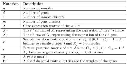
Suppose our gene expression matrixX containsdgenes and nsamples, and we would like to group the genes intomclusters and group the samples intocclusters (cancer subtypes). For convenience, the main notations used in the rest of the thesis are presented in Table1.

Table 1: Main notations Notation Description

n Number of samples

d Number of genes

c Number of sample clusters

m Number of gene clusters

X Gene expression matrix of sized×n

X·i Theithcolumn ofX, representing the expression of theithsample Xi· Theithrow ofX, representing the expression of theithgene

F Sample partition matrix of sizen×c;Fij ∈[0,1] : Fij = 1 ifX·i

belongs to sample clusterj andFij= 0 otherwise

G Feature partition matrix of size d×m; Gij ∈[0,1] : Gij = 1 if Xi·belongs to gene clusterj andGij = 0 otherwise

S Am×cmatrix

W Ad×ddiagonal matrix; entries are the weights of the genes

Our method can be specified as minimizing the following objective,

kX−GSFTk2 W = d X i=1 kXi·−(GSFT)i·k2×Wii = tr(XTW X−2XTW GSFT +F STGTW GSFT). (2.7)

Here G denotes the cluster each gene belongs to and F denotes the cluster of each sample. The matrix S can be treated as centroids of the bi-clusters (blocks in heatmap) generated. Weights trained before are presented in the diagonal matrixW, and we incor-porate this importance indicator by multiplying the weights to the squared row (genes)

norms. Therefore, in the optimization step, genes with larger weights contribute more and have higher priority. IfW =I, i.e. all the genes have same weight 1 and are treated equally, it degenerates to the ordinary co-clustering method. Due to difficulties in minimizing the objective with the binary-value constraint onF andG, we relaxF and Ginto continuous nonnegative domain as in previous related work (Gu and Zhou, 2009). We only require Pm

j=1Gij = 1,

Pc

j=1Fij= 1. Thus our objective is to minimize:

J = tr(XTW X−2XTW GSFT +F STGTW GSFT), s.t.G≥0, F ≥0, m X j=1 Gij = 1, c X j=1 Fij = 1. (2.8)

2.3.2

Optimization

entries represent the number of samples belonging to each sample cluster, andGT_{W Gshould}

be am×mdiagonal matrix, with entries equal to the total weights of features (genes) belong-ing to each of themfeature (gene) clusters; similarly to the interpretation ofFT_F,GT_{W G}

can be considered as the weighted total number of features in each feature cluster (taking feature i as wi features when counting the total number). Therefore, (GTW G)−1GTW X

represents the feature cluster centroids on the sample space (n-dimension) andXF(FTF)−1 represents the sample cluster centroids on the feature space (d-dimension). The difference is that all the samples are assumed to have same weights equal to 1 while feature points are assigned different weightsW. S then can be viewed as feature cluster centroids on the sample-centroids space (c-dimension) or as sample cluster centroids on the gene-centroids space (m-dimension). Therefore, it gives the centroids information of the bi-clusters (m×c) after partitioning.

Lagrangian function forF is

L(F) =J−tr(βFT). (2.11)

We set:

∂L(F)

∂F = 0. (2.12)

Using Karush-Kuhn-Tucker condition (Boyd and Vandenberghe,2004), we have

(−A++A−+F B+−F B−)ijFij = 0, (2.13)

where A = XTW GS, B = STGTW GS; M+ and M− are the positive and negative of matrixM defined as M+ = |M|₂+M,M− = |M|−₂M, respectively. Therefore, we obtain the iterating formula forF:

Fij ←Fij s (A+_{+F B}−₎ ij (A−_{+F B}+₎ ij . (2.14)

Similar derivation leads to the iterative formula ofG:

Gij ←Gij s (C+_{+W GD}−₎ ij (C−_{+W GD}+₎ ij , (2.15) whereC=W XF ST_,D=SFT_{F S}T_.

The iterations decrease the value of the objective function, J. We include the proof of convergence of this algorithm in the following section.

Therefore, our algorithm is as follows: • Initialize F andG.

• While not convergent and iterations less than a pre-defined value – UpdateS by S= (GTW G)−1GTW XF(FTF)−1; – UpdateF by Fij ←Fij s (A+_{+F B}−₎ ij (A−_{+F B}+₎ ij ; – UpdateGby Gij←Gij s (C+_{+W GD}−₎ ij (C−_{+W GD}+₎ ij .

2.3.3

Proof of convergence

We use the auxiliary function approach to prove the convergence of our algorithm.

Z(h, h0) is called an auxiliary function forF(h) ifZ(h, h0)≥F(h) andZ(h, h) =F(h). Leth(t+1)_{= arg min}

hZ(h, h(t)), thenF(h(t+1))≤Z(h(t+1), h(t))≤Z(h(t), h(t))≤F(h(t)).

Lemma 1. For any matricesU ∈Rk+×k, M, M0 ∈R

n×k

+ , if U is symmetric, the following

inequality holds: n X i=1 k X j=1 (M0U)ijMij2 M_ij0 ≥tr(M T_{M U). (2.16)} Proof. LetMij =vijMij0 . LHS= n X i=1 k X j,l=1 M_il0UljMij0 v 2 ij= n X i=1 k X j,l=1 M_il0UljMij0 v2 ij+vil2 2 . RHS = n X i=1 k X j,l=1 vilMil0vijMij0 Ujl= n X i=1 k X j,l=1 M_il0UljMij0 vijvil. Therefore, LHS−RHS= n X i=1 k X j,l=1 Mil0UljMij0 (vij−vil)2 2 ≥0.

For any real-valued matrix A, defineA+₌|A|+A

2 , A

−₌ |A|−A

2 .

Theorem 1. LetJ(M) =tr(−2P MT_{+M QM}T_{), whereP ∈}

Rn×k andQ∈Rk×k are fixed

matrices, and Qis symmetric,M ∈_Rn×n_{. Then} Z(M, M0) =−2X i,j P_ij+M_ij0 (1 + logMij M_ij0 ) + X i,j P_ij−M 2 ij+Mij0 2 2M_ij0 +X i,j (M0Q+)ijMij2 M_ij0 − X i,j,l Q−_jlMij0 Mil0(1 + log MijMil M_ij0 M_il0 ) (2.17) is an auxiliary function ofJ(M).

Furthermore, fixing M0, Z(M,M’) is a convex function ofM and it has the global mini-mum at Mij =Mij0 v u u t P_ij++ (M0_Q−₎ ij P_ij−+ (M0_Q+₎ ij (2.18)

Proof. ∀x∈R+, 1 + logx≤x =⇒ P_ij+M_ij0 (1 + logMij M_ij0 )≤P + ijMij; Q−jlM 0 ijMil0(1 + log MijMil M_ij0 M_il0 )≤Q − jlMijMil a2+b2≥2ab =⇒ P_ij−M 2 ij+Mij0 2 2Mij ≥P_ij−Mij. Lemma1 =⇒ (M 0_Q+₎ ijMij2 M0 ij ≥tr(MTM Q+). Therefore, Z(M, M0)≥ −2tr(P+MT) + 2tr(P−MT) +tr(MTM Q+)−tr(M Q−MT) =J(M).

To find the minimum of Z(M, M0_{), we take}

∂Z ∂Mij =−2P_ij+M 0 ij Mij + 2P_ij−Mij M_ij0 + 2 (M0Q+₎ ijMij M_ij0 −2 (M0Q−)ijMij0 Mij , ∂2_Z ∂Mij∂Mlm =δilδjm(2Pij+ M_ij0 M2 ij + 2P − ij M0 ij + 2(M 0_Q+₎ ij M0 ij + 2(M 0_Q−₎ ijMij0 M2 ij )≥0.

Therefore,Z(M, M0) is a convex function ofM. Let _∂M∂Z ij = 0, we haveMij =M 0 ij r P+ ij+(M0Q−)ij P_ij−+(M0_Q+_)ij.

Therefore, arg minMZ(M, M0) has entriesMij0

r

P+

ij+(M0Q−)ij P_ij−+(M0_Q+_)ij.

LetP =XTW GS =A, Q=STGT W GS=B and M =F, we can see that updating

F using Fij =Fij v u u t A+_ij+ (F B−₎ ij A−_ij+ (F B+₎ ij (2.19) monotonically decreases the value of the objective functionJ in the method part. Besides, we know thatJ ≥0, so the updating algorithm converges. Since W is a diagonal matrix with positive entries, we can similarly letP =XF ST _=W−1_{C, Q=SF}T_{F S}T _{=D and} M =G, so updatingGusing Gij =Gij v u u t C_ij++ (W GD−₎ ij C_ij−+ (W GD+₎ ij =Gij v u u t (W−1_C)+ ij+ (GD−)ij (W−1_C)− ij+ (GD+)ij (2.20)

algorithm converges.

2.3.4

m

and

c

selection

A question raised in almost all clustering methods is how to determine the cluster numbers. There is no agreed-upon solution. Here we utilize an approach taking advantage of the stochastic property of the algorithm: NCIS may not converge to the same solution on each run with different initiation; however, if the clustering is strong enough, we would expect that the results of multiple runs would be very stable (Brunet et al.,2004; Monti et al.,2003). As in (Brunet et al.,2004;Monti et al.,2003), we run NCIS for 50 times with randomly-set initiations and get a sample consensus matrixMsand a gene consensus matrix Mg. For each run, a n×nsample connectivity matrix Ms and a d×dgene connectivity

matrixMg are obtained.

Ms(i, j) =     

1 if Samplei and Samplej belong to the same cluster 0 otherwise (2.21) Mg(i, j) =     

1 if Geneiand Genej belong to the same cluster 0 otherwise

(2.22)

Consensus matrices Ms and Mg are the averages of Ms’s and Mg’s over the 50 runs

respectively. The entries would range between 0 and 1, where 0 indicates that the corre-sponding samples (genes) belong to different clusters in every run and 1 indicates that they belong to the same clusters in all the cases. Therefore, 1−M offers a new distance metric evaluating the similarity of the items (1−Msfor samples and 1−Mg for genes). Similar to

(Brunet et al.,2004), we use 1−Msand 1−Mgto hierarchically cluster samples and genes,

and then we define an average cophenetic correlation coefficient ρ(Ms)+ρ(Mg)

2 to evaluate

the stability over 50 runs. Cophenetic correlation coefficient ρ of matrix C is defined as the Pearson correlation between distance matrix 1−C and the distance matrix induced by the linkage used in hierarchical clustering for re-ordering C. If a clustering is stable, the entries would be close to 0 and 1 (two modes), and in the ideal case (only 0 and 1) the average cophenetic correlation coefficient would be exactly 1. So we observe how the cophenetic correlation coefficients change as m and c change, and select point where the averaged coefficient begins to fall.

Chapter 3

Results

We applied NCIS to two large-scale datasets from TCGA. We also used simulated datasets to evaluate the effectiveness of our method. The network was built using a variety of sources, including the network used in (Ciriello et al., 2012) as well as our up-to-date curated information from Reactome (Croft et al., 2011), the NCI-Nature Curated PID (Schaefer et al., 2009), and KEGG (Kanehisa et al., 2012). The resulting aggregated network consisted of 11,648 genes and 211,794 edges. For some gene pairs, we can just tell a connection between them but not able to identify the direction of the regulation, so we assign two links with opposite directions between them. We allow users to input other network information in the MATLAB implementation of our method.

3.1

Breast Cancer Dataset

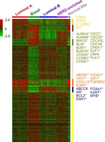
The first dataset we used is from a recent large-scale breast cancer study done by TCGA (Network, 2012). This dataset contains the expression of 17,814 genes across 547 samples. We first integrated the gene expression profile with the network information, and trained weights for 8,726 genes included in both resources. In this step, we setα= 0.85. The 8,726 weighted genes and 547 samples were the input of the co-clustering algorithm. Figure 2

shows the heatmap with genes and samples rearranged according to the clustering result. Based on the cophenetic correlation coefficient calculated from 50 runs (see Method part), we chosec= 5 andm= 8 (data shown in Table2).

Since we do not know the true class each sample belongs to or even how many subtypes there are, we used clinical features to evaluate the effectiveness of the clustering algorithm. The underlying idea is that patients in different subgroups are expected to have distinct clinical characteristics. In addition, as the goal of cancer subtype detection is to assist diag-nostic of the disease and designing more specific and targeted treatment, a good clustering

Table 2: Cophenetic coefficients for BRCA data m= 6 m= 7 m= 8 m= 9 c= 4 0.931 0.925 0.930 0.944 c= 5 0.930 0.940 0.948 0.942 c= 6 0.924 0.929 0.945 0.947 c= 7 0.926 0.928 0.942 0.937

c for number of subtypes, m for number of gene clusters.

result need to reflect certain clinical information.

Luminal ABasal Luminal B HER2-enriched Normal-like CDK6* EGFR* IL12RB2 KIT* AURKA* AURKB* BIRC5* BLM* BUB1* BUB1B* CCNA2* CCNB2* CCNE1* ABCB1* CAV1* CXCL12* EGR1* ABCC8 AR* BCL2* ESR1* 2.0 -2.0 0 CDC2* CDC20* CDC45L CDCA8 CHEK1* E2F1* LRP8 PLK1* FOXO1* IGF1* TGFBR2* FOXA1* IL6ST* MYB*

Figure 2: Heatmap of breast cancer expression data. Samples and genes rearranged according to our NCIS results. Genes listed are the 35 genes used to train classifier. Genes with “*” are those previously reported to be associated with breast cancer.

We used the following clinical information to evaluate subtypes identification result: sur-vival time, age at initial pathologic diagnosis, AJCC staging information (neoplasm disease lymph node stage, neoplasm disease stage and tumor stage) and tumor nuclei percentage.

Given p-value threshold 0.05, we can conclude that the NCIS-defined subtypes successfully separated the patients according to all of these clinical features.

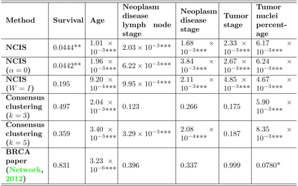
Table 3: P-value of the dependence test for different clinical features and BRCA subtypes

Method Survival Age

Neoplasm disease lymph node stage Neoplasm disease stage Tumor stage Tumor nuclei percent-age NCIS 0.0444** 1.01 × 10−3_*** 2.03×10−3*** 1.68 × 10−3_*** 2.33 × 10−3_*** 6.17 × 10−3_*** NCIS (α= 0) 0.0442** 1.96 × 10−3*** 6.22×10 −3_*** 3.84 × 10−3*** 2.67 × 10−3*** 6.24 × 10−3*** NCIS (W =I) 0.195 9.20 × 10−4_*** 9.95×10−4*** 2.11 × 10−3_*** 4.85 × 10−3_*** 4.67 × 10−3_*** Consensus clustering (k= 3) 0.497 2.04 × 10−3_*** 0.123 0.266 0.175 5.90 × 10−3_*** Consensus clustering (k= 5) 0.359 3.40 × 10−3_*** 3.29×10−3*** 2.08 × 10−4_*** 0.187 8.35 × 10−3_*** BRCA paper (Network, 2012) 0.831 3.23 × 10−6_*** 0.396 0.337 0.999 0.0780*

For survival time, we used logrank test; for AJCC neoplasm disease lymph node stage, AJCC neoplasm disease stage and AJCC tumor stage, we used Chi-squared test; for tumor nuclei percentage and age at initial pathologic diagnosis, we used ANOVA. In all the 547 samples, there are 22 tumor-adjacent normal tissue samples. They were assigned to same subtypes by all the clustering methods we used. We ignored these “normal” subtypes in the clinical feature tests, as these subtypes contain few samples after the 22 normal ones were excluded. * for p <0.1, ** forp <0.05, *** forp <0.01.

We also setα= 0 in the co-clustering method, i.e. no network information was used, to see the impact of network structure in the clustering results. Similar statistical tests were performed and the results were presented in Table3. Comparing the p-values under the two methods, we did observe an improvement with network information added, in separation of all the clinical features.

In the original paper (Network,2012), the authors performed a hierarchical clustering using a subset of genes (most varied across samples) and identified 13 subtypes (test results for clinical features are shown in Table 3 as BRCA paper). Since consensus hierarchical clustering generally performs better than the traditional hierarchical clustering, we applied a consensus average linkage hierarchical clustering (Monti et al.,2003;Wilkerson and Hayes,

2010) to cluster the samples. To make a fair comparison, we used all the 8,726 genes. The program was run over 1,000 iterations and the resampling rate of the sample was set to be 0.8. The distance metric is 1 minus Pearson’s correlation coefficient. The algorithm suggested 3 subtypes be identified. However, in Table 3, we listed the tests p-values of both 3-subtypes and 5-subtypes conditions to make it easier to compare with the results of NCIS. The results indicated that in the perspective of all these clinical characteristics except for AJCC neoplasm disease stage, clusters generated by consensus clustering are not as informative as those of NCIS. We think the most important reason for the poorer performance of consensus clustering is a lack of effective feature selection method. Consensus clustering is well designed itself, however, when there are a large number of genes included in the expression profile, the users must first filter out non-informative ones before performing the clustering, otherwise the true signals will be weakened by strong noises.

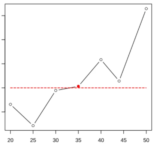
The major advantages of NCIS is the incorporation of the network structure and as-signing an importance indicator to each gene, so besides generating the co-clusters, we also obtained a bi-product – the gene weights, which describe the genes’ roles in the network and abilities to distinguish the patients. After getting the subtypes, we trained a classifier so that when a new patient is diagnosed, we can easily predict his/her subtype based on the ex-pression levels of a few signature genes. We first selecting out 35 genes (shown in Figure2): we performed ANOVA tests for each gene’s expression levels across the five subtypes, and then chose the first 35 genes with largest weights and smallest p-values. We constructed a classifier based on SVM with these 35 genes. In order to test the performance of this classifier, we performed 10-fold cross validation on this BRCA dataset for 20 times. In this step, we also tried to use other numbers of genes as classification features. We collected the average 10-fold cross validation accuracy (20 times) for each case. We chose 35 because it is the smallest number that can give an accuracy larger than 0.90 (Figure3). After evaluating the accuracy with 10-fold cross validation, we trained a classifier using all the 547 samples (35 genes). We used this classifier to predict the subtypes of these 547 sample in turn. The accuracy is 0.978.

We tested the functions of these 35 genes. They are enriched in pathways related to cell cycle, cell division, etc. (Table4, from DAVID (Huang da et al.,2009a,b)). According to GeneCards (www.genecards.org) (Safran et al.,2010), all these genes are highly associated with breast cancer based on previous publications, except for CDCA8, ABCC8, CDC45L,

● ● ● ● ● ● ● 20 25 30 35 40 45 50 0.89 0.90 0.91 0.92 0.93 #genes Accur acy ●

Figure 3: Accuracies of BRCA subtype classifiers trained with different numbers of genes. Genes with largest weights and largest expression differences were used.

IL12RB2 and LRP8. However, CDCA8 encodes a protein relevant to mitosis and cell division regulation; ABCC8 is involved in multi-drug resistance; CDC45L is required for initiation of chromosomal DNA replication; IL12RB2 is related to immune response; LRP8 is the cell receptor of Reelin and Reelin has been reported to be important in controlling invasiveness and metastatic potential of breast cancer cells (Stein et al.,2010). Therefore, these five genes might also play a role in breast cancer.

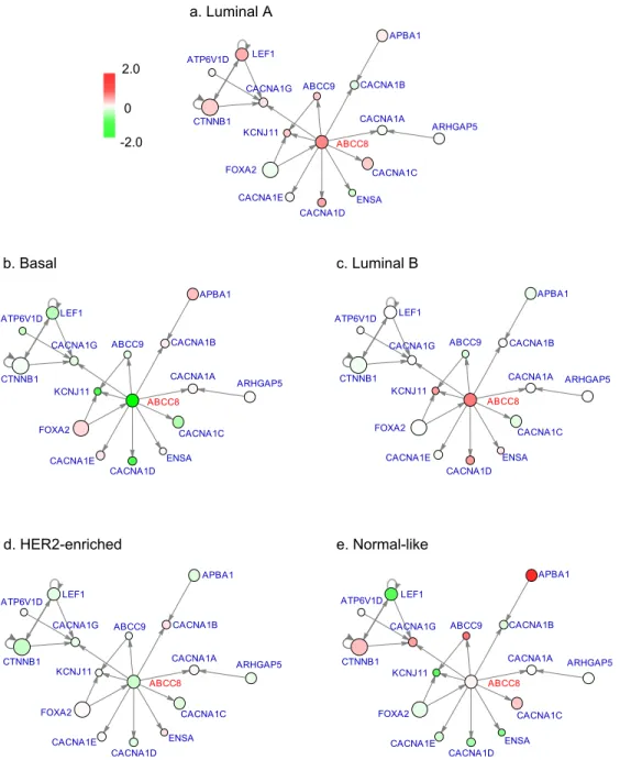
We extracted the subnetwork of ABCC8 as an example to illustrate the differences of the five subtypes in network level (Figure 4). There are 9 genes targeted by ABCC8 in the network we used. We chose this subnetwork because it has a small size and is easy to be presented clearly. As can be seen from Figure 4, ABCC8 is highly expressed in Subtypes Luminal A and Luminal B. Its downstream gene KCNJ11 has very similar expression pattern with it: KCNJ11 is also highly expressed in Luminal A and Luminal B, but has very low expression levels in the other three subtypes where ABCC8 is less expressed. There are many other such examples, which further confirm the differential expression pattern between subtypes in network level – a main assumption of our method.

As PAM50 (Parker et al., 2009) is widely used in breast cancer subtype detection, we compared the results of our classifier with that from PAM50 (Network,2012;Parker et al.,

2009). For these 547 samples, 372 of them (68%) have same subtypes predicted by both PAM50 and our classifier (p-value for chi-squared test 10−10 _{(Network, 2012)). This}

Table 4: Pathways enriched by BRCA 35 genes Term P-value Cell cycle 5.45×10−19 Oocyte meiosis 5.05×10−15 Pathways in cancer 1.23×10−14 Prostate cancer 3.40×10−11 p53 signaling pathway 1.11×10−9

Progesterone-mediated oocyte maturation 3.59×10−9

Cytokine-cytokine receptor interaction 7.59×10−7

Glioma 1.15×10−5

Melanoma 1.75×10−5

Pancreatic cancer 1.90×10−5

Small cell lung cancer 2.71×10−5

Colorectal cancer 3.02×10−5

Focal adhesion 3.55×10−4

Non-small cell lung cancer 6.43×10−4 Chronic myeloid leukemia 1.30×10−3

Endocytosis 5.12×10−3

ABC transporters 0.0163

Bladder cancer 0.0290

p-value<0.05, results from DAVID.

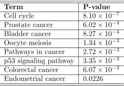
concordance further supports that our method provides a pipeline which can be very useful in cancer subtype prediction. By comparing the genes used in the two classifiers, we found there are 7 genes overlapped. Although the remaining genes are different, their functions are similar. According to DAVID (Huang da et al.,2009a,b), PAM50’s 50 genes are also enriched in pathways related to cell cycle, cell division, etc. (Table5).

Though the results of NCIS-derived classifier and PAM50 were highly consistent globally, we further investigated samples that were assigned different class labels by the two methods. We focused on the expression values of 100 top-ranked genes as these genes were considered most important in our clustering method. We got the median expression levels of these genes for each subtype using the samples that were categorized into this specific subtype by both methods (this subtype information we think should be reliable), and then compared expression levels of samples that were predicted to different subtypes with these median values. In this comparison, only 53 samples (30.1%) have expression profiles more similar to PAM50-predicted subtypes.

In summary, we conclude that NCIS can detect breast cancer subtypes very reliably. Besides, it also provides an effective approach to train a classifier that can be used for dialogistic purpose.

CTNNB1 LEF1 ABCC8 ABCC9 CACNA1A CACNA1B CACNA1C CACNA1D CACNA1E CACNA1G ENSA KCNJ11 FOXA2 ARHGAP5 APBA1 ATP6V1D CTNNB1 LEF1 ABCC8 ABCC9 CACNA1A CACNA1B CACNA1C CACNA1D CACNA1E CACNA1G ENSA KCNJ11 FOXA2 ARHGAP5 APBA1 ATP6V1D CTNNB1 LEF1 ABCC8 ABCC9 CACNA1A CACNA1B CACNA1C CACNA1D CACNA1E CACNA1G ENSA KCNJ11 FOXA2 ARHGAP5 APBA1 ATP6V1D CTNNB1 LEF1 ABCC8 ABCC9 CACNA1A CACNA1B CACNA1C CACNA1D CACNA1E CACNA1G ENSA KCNJ11 FOXA2 ARHGAP5 APBA1 ATP6V1D CTNNB1 LEF1 ABCC8 ABCC9 CACNA1A CACNA1B CACNA1C CACNA1D CACNA1E CACNA1G ENSA KCNJ11 FOXA2 ARHGAP5 APBA1 ATP6V1D 2.0 -2.0 0 a.mLuminalmA b.mBasal c.mLuminalmB d.mHER2-enriched e.mNormal-like

Figure 4: Expression patterns of ABCC8 subnetwork in BRCA subtypes. Genes directly connected to ABCC8 and genes targeting ABCC8’s downstream genes are included. Color of circle corresponds to gene expression level; size of circle corresponds to gene weight. a. Subtype Luminal A; b. Subtype Basal; c. Subtype Luminal B; d. Subtype HER2-enriched; e. Subtype Normal-like.

3.2

Glioblastoma Dataset

The second dataset we used is from a large-scale Glioblastoma multiforme (GBM) subtype identification work (Verhaak et al.,2010). The authors integrated data generated on three

Table 5: Pathways enriched by PAM50 50 genes Term P-value Cell cycle 8.10×10−7 Prostate cancer 6.02×10−4 Bladder cancer 8.27×10−4 Oocyte meiosis 1.34×10−3 Pathways in cancer 2.72×10−3 p53 signaling pathway 3.35×10−3 Colorectal cancer 6.07×10−3 Endometrial cancer 0.0226 p-value<0.05, results from DAVID.

platforms into a single dataset using factor analysis. This unified dataset contains the expression of 11,861 genes on 200 GBM and 2 normal brain samples. In the original paper, the authors first selected 1,903 variably expressed genes according to the MAD and then applied consensus hierarchical clustering with agglomerative average linkage (Monti et al.,

2003). Four subtypes were detected.

We integrated the gene expression information with the network information to train a weight for each of the 7,183 genes included in both sets. Tuning parameter α in the algorithm was set to be 0.85. After obtaining the weights, these 7,183 weighted-genes and the 202 samples were used in the co-clustering. We set m = 7 and c = 4. The cluster numbers were chosen in the way described in the method section (Table6).

Table 6: Cophenetic coefficients for GBM data

m= 6 m= 7 m= 8 m= 9

c= 4 0.911 0.920 0.904 0.916

c= 5 0.903 0.904 0.906 0.899

c= 6 0.902 0.892 0.902 0.894

c for number of subtypes, m for number of gene clusters.

Since we do not have a “gold standard” for the clustering results here either, we used clinical characteristics to evaluate the effectiveness of our method again. From all the clinical features provided in this dataset, we used survival time, age at first diagnosis, tumor necrosis percentage, and tumor nuclei percentage.

Table7gives the significance level of the difference among all subtypes for each feature. Given a p-value threshold 0.05, NCIS results separated the samples in their survival time,

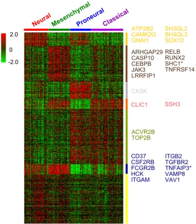
2.0 -2.0 0 NeuralMesen chymal ProneuralClassical ATP2B2 CAMK2G GNAI1 ARHGAP29 CASP10 CEBPB JAK3 LRRFIP1 SH3GL2 SH3GL3 SOX10 RELB RUNX2 SHC1* TNFRSF14 CASK CLIC1 SSH3 ACVR2B TOP2B CD37 CSF2RB FCGR2B HCK ITGAM ITGB2 TGFBR2 TNFAIP3* VAMP8 VAV1

Figure 5: Heatmap of GBM expression data. Rearranged according to our NCIS results. Genes listed are the 30 genes used to train classifier. Genes with “*” are those previously reported to be associated with glioblastoma.

tumor necrosis percentages and tumor nuclei percentages very well. Besides, the ages at first diagnosis also showed difference to a certain extent. Therefore, we think NCIS performs well on this dataset in detecting clinically distinct GBM subtypes. Interestingly, we also observed that Subtype Pronueral has a much higher survival rate than the other three subtypes (Figure6). The underlying mechanism for this significant difference deserves more study.

We also used consensus average linkage hierarchical clustering (Monti et al., 2003;

Wilkerson and Hayes,2010), as the author did in the paper, but on the 7,183-gene dataset, to cluster the samples. The program was run over 1,000 iterations and the resampling rate of the sample was set to be 0.8. The distance metric is 1 minus Pearson’s correlation coefficient. We identified 4 clusters among the patients. According to the p-values, NCIS-defined subtypes separated the patients in their survival time, age of first diagnosis and tumor nucleic percentages much better.

Table 7: P-value of the dependence test for different clinical features and GBM subtypes

Method Survival Age Tumor necrosis

percentage Tumor nuclei percentage NCIS 0.0241** 0.0608* 1.14×10−4*** 3.26×10−3*** NCIS (α= 0) 0.0140** 0.0278** 3.29×10−4_{*** 4.28×10}−3_*** NCIS (W =I) 0.0321** 0.0402** 1.70×10−3_{*** 2.37×10}−3_*** Consensus clus-tering (k= 4) 0.101 0.124 1.09×10 −4_{*** 0.0105**} GBM paper (Verhaak et al., 2010) 0.153 0.0135** 3.25×10−5_{*** 8.80×10}−3_***

For survival time, we used logrank test; for tumor necrosis percentage, tumor nuclei percentage and age at initial pathologic diagnosis, we used ANOVA. * forp <0.1, ** forp <0.05, *** forp <0.01.

We trained a classifier based on the first 30 genes (shown in Figure 5) with highest weights and largest expression differences between subtypes. Like what we did in BRCA data analysis, we also used different numbers of genes to train classifier and got accuracy estimations based on the average accuracy of 10-fold cross validation for 20 times. We selected a smallest number of genes which can give accuracy higher than 0.90 (Figure 7). After evaluating the accuracy with 10-fold cross validation, we trained a classifier using all the 202 samples (30 genes), and then used this classifier to predict the subtypes of these 202 sample in turn. The accuracy we got is 0.960.

We tested the functions of the 30 genes used in the classifier. According to DAVID (Huang da et al., 2009a,b), they are enriched in pathways related to immune response, endocytosis, apoptotic process, etc. (Table 8). These functions were reported to play im-portant roles in cancer progression. For example, derailed endocytosis of surface receptors can abnormally regulate crucial features of signal transduction (Hanahan and Weinberg,

2000;Mosesson et al.,2008); loss of apoptosis can disrupt the balance between cell prolif-eration and cell death and lead to cancer (Fesik,2005).

We also extracted a subnetwork to illustrate the difference between subtypes in network level. Here we considered gene C1QA (Figure 8), which is involved in immune response (GeneCards, (Safran et al., 2010)). We selected this subnetwork because it has a compact structure. As can be seen from Figure 8, downstream targets like C1QB and C2 have very similar expression pattern with C1QA. However, cases are more complicated for genes like IGKV1-5 and IGKC. We think this is due to the large number of upstream genes for

0 500 1000 1500 2000 2500 3000 3500 0.0 0.2 0.4 0.6 0.8 1.0 Days Sur viv al Normal Mysenchymal Proneural Classical a.bNCIS b.bNCISbkα=0G c.bNCISbkW=IG d.bConsensusbClusteringbkk=4G e.bGBMbPaper 0 500 1000 1500 2000 2500 3000 3500 0.0 0.2 0.4 0.6 0.8 1.0 Days Sur viv al 0 500 1000 1500 2000 2500 3000 3500 0.0 0.2 0.4 0.6 0.8 1.0 Days Sur viv al 0 500 1000 1500 2000 2500 3000 3500 0.0 0.2 0.4 0.6 0.8 1.0 Days Sur viv al 0 500 1000 1500 2000 2500 3000 3500 0.0 0.2 0.4 0.6 0.8 1.0 Days Sur viv al

Figure 6: Kaplan-Meier survival curves of GBM data. Red for Subgroup Neural, green for Mesenchymal, blue for Proneural and purple for Classical; horizontal axis is the survival time (days) and vertical axis is the survival rate). a. NCIS-defined subtypes; b. NCIS (α= 0) defined subtypes; c. NCIS (W =I) defined subtypes; d. Consensus clustering (k= 4) defined subtypes; e. GBM paper defined subtypes.

● ● ● ● ● ● ● 20 25 30 35 40 45 50 0.88 0.89 0.90 0.91 #genes Accur acy ●

Figure 7: Accuracies of GBM subtype classifiers trained with different numbers of genes. Genes with largest weights and largest expression differences were used.

Table 8: Pathways enriched by GBM 30 genes

Term P-value

Chemokine signaling pathway 2.76×10−6

Leukocyte transendothelial migration 3.71×10−5 Regulation of actin cytoskeleton 2.19×10−4

Cytokine-cytokine receptor interaction 3.42×10−4 Fc gamma R-mediated phagocytosis 1.27×10−3

Natural killer cell mediated cytotoxicity 2.08×10−3

Endocytosis 3.62×10−3

Glioma 0.0364

B cell receptor signaling pathway 0.0427

Chronic myeloid leukemia 0.0452

Hematopoietic cell lineage 0.0489 TGF-beta signaling pathway 0.0495

Apoptosis 0.0495

p-value<0.05, results from DAVID.

3.3

Simulated Datasets

To better evaluate the accuracy of NCIS, we simulated a set of expression profiles composed of 300 samples and 3 subgroups. The gene expression values were generated according to the real expression profile in the BRCA dataset (Network,2012).

We assume for sample i in subgroup k, gene expression x·i ∼ N(µk, Σ), whereµk is

a column vector representing the mean expression levels for subgroupk, and Σ is used to model the network structure and the variance within subtype. To estimate Σ, we used

HLA−B HLA−C HLA−F HLA−G CXCR4 CD79A HLA−DMA IGHM C1QA C1QB C1S C2 CR1 IGKC IGKV1−5 IGLV2−14 C3 C5 CD55 FCGR2B CD40LG HLA−B _HLA−C HLA−F HLA−G CXCR4 CD79A HLA−DMA IGHM C1QA C1QB C1S C2 CR1 IGKC IGKV1−5 IGLV2−14 C3 C5 CD55 FCGR2B CD40LG HLA−B HLA−C HLA−F HLA−G CXCR4 CD79A HLA−DMA IGHM C1QA C1QB C1S C2 CR1 IGKC IGKV1−5 IGLV2−14 C3 C5 CD55 FCGR2B CD40LG HLA−B _HLA−C HLA−F HLA−G CXCR4 CD79A HLA−DMA IGHM C1QA C1QB C1S C2 CR1 IGKC IGKV1−5 IGLV2−14 C3 C5 CD55 FCGR2B CD40LG 2.0 -2.0 0 d.iClassical c.iProneural b.iMesenchymal a.Neural

Figure 8: Expression patterns of C1QA subnetwork in GBM subtypes. Genes directly connected to C1QA and genes targeting C1QA’s downstream genes are included. Color of circle corresponds to gene expression level; size of circle corresponds to gene weight. a. Subtype Neural; b. Subtype Mesenchymal; c. Subtype Proneural; d. Subtype Classical.

graph Laplacian of the network. We first obtained an adjacency matrix ˜Afrom the original network matrixE: ˜A= max(E, E0), where E0 is the transposal ofE. The degree matrix

˜

D is defined as a diagonal matrix with entries equal to the sum of the corresponding rows of ˜A. The graph Laplacian is thusL= ˜D−A˜. We estimated Σ as:

Σ =ν(I−D˜−12A˜D˜− 1

2). (3.1)

The main idea is that expression levels of genes connected in the network structure would be correlated. Here we assume the correlations are proportional to the proximities in the network. We use this technique to simulate datasets so interactions between genes

can be considered. To determine constantν, we compared the diagonal entries of matrix

I−D˜−1 2A˜D˜−

1

2 (expression variances) and the variances of real gene expression levels in the

BRCA dataset. In our simulation, we setν= 0.5.

For the three subtypes we simulated here, the mean expression levels of each gene were estimated from the gene expression profiles of Luminal A, Basal and Luminal B detected in the BRCA dataset. The final simulated datasets contain 300 samples and 8,726 genes.

Some noises were added to the datasets, otherwise the signal would be too strong. We first trained a weight for each gene based on only the network structure (α= 1 in the weight-training algorithm) and then choselgenes with lowest weights to be “noninformative” genes: we randomly permutated the expression levels of these genes across the samples. l was set to be 1,000, 2,000, 3,000, 4,000 and 5,000 to illustrate the influence of noises. We generated 5 datasets for eachl.

We setm= 8 andc= 3 in NCIS. The results for multiple trials of the simulation studies were shown in the Table9. We also included the results for consensus clustering here. As we can see, when the number of “noisy” genes is small (1000 and 2000), both methods have 100% accuracy; when there are 3000 noises, NCIS begins to perform better than consensus clustering. However, if there are too many noises (5000), neither method can have very good prediction. Considering that the total number of genes used here is less than 9000, this poor performance is acceptable. Overall, our simulation studies indicate that NCIS is a robust method that can detect cancer subtypes very accurately.

Table 9: Clustering accuracies on simulated datasets

#“noisy” Case 1 Case 2 Case 3 Case 4 Case 5

genes NCIS Cons NCIS Cons NCIS Cons NCIS Cons NCIS Cons 1000 1.000 1.000 1.000 1.000 1.000 1.000 1.000 1.000 1.000 1.000 2000 1.000 1.000 1.000 1.000 1.000 1.000 1.000 1.000 1.000 1.000 3000 1.000 0.913 0.997 0.887 0.907 0.897 1.000 0.877 1.000 0.870 4000 1.000 0.797 0.720 0.673 0.807 0.727 1.000 0.680 0.703 0.703 5000 0.710 0.633 0.573 0.573 0.680 0.547 0.613 0.613 0.677 0.567 For each given number of “noisy” genes, we simulated 5 datasets (Case 1-5).

Chapter 4

Conclusion

Cancer subtype information is of critical importance in designing better treatment strategy. In this work, we aim at developing a clustering method that can help identify cancer subtypes from high-throughput gene expression data and select subtype-related gene sets. We propose a new co-clustering method that incorporates the network information within the clustering step to detect biologically informative sample subtypes and co-expressed gene sets. The main rationale underlying our method is as follows. First, genes playing key roles in network should be more emphasized than down-stream target genes; therefore we assign a weight to each gene based on its connectivity in network and the distinguishing ability in expression level across all samples. This weight also serves as a natural feature selection criterion since key genes will be more favored in the clustering algorithm. We also avoid excluding a large number of genes using this kind of feature selection. Less information loss should be beneficial for subsequent analysis. Second, a co-clustering method can better capture the duality of gene expression profiles, in terms that similarity is treated as a level of coherence of the samples and genes in the bi-clusters; thus we construct the model based on a co-clustering method, SNMTF, considering its intuitive meaning and its ability to handle gene expression dataset. We search for the minimum of the objective through iterative algorithms. Since our method takes prior knowledge on network structure to guide the clustering, we expect that the clustering results would be more biologically relevant and more resistant to the spurious similarities, compared to subtypes clustering methods only based on the expression matrix. We tested our method on two large-scale expression profiles and several simulated datasets. We were able to detect distinct subtypes that are biologically meaningful in both real datasets and to cluster most samples correctly in the simulated ones. These results suggested that our method provides a unique solution to cancer subtype identification based on gene expression profiles.

molecular interaction network, i.e., it is not specific for the particular type of cancer or the tissue used in the experiment. Second, the network does not contain all the genes, so some genes were excluded simply because we cannot assign a comparable weight for it. Third, a lot of edges in our current network do not have high confidence level and the directions of many edges are unclear. These three problems are mainly due to a lack of complete pictures on gene-gene interaction mechanisms, especially cancer-specific or tissue-specific network information. A possible approach dealing with the first two network problems is to update the network information according to the expression patterns. The “posterior” network generated could be more specific and guide the clustering better. Besides, with more knowledge accumulated on gene network, we believe the performance of our method can be further improved. In addition, we think the gene weights trained from NCIS could be applied to the consensus clustering for feature resampling. Consensus clustering outperforms many conventional methods since it integrates the results across multiple runs of a regular clustering on subsets of samples. However, our result indicated that its robustness decreased as the dimension became large. Therefore, a proper weight input for resampling the features may help in selecting more informative genes. This modified version of consensus clustering can also be integrated with co-clustering frameworks.

Overall, we believe our new NCIS method will be highly useful to comprehensively identify subtypes that are otherwise obscured by cancer heterogeneity, from various types of cancers based on high-throughput and high-dimensional gene expression data.

References

Alizadeh, A. A., Eisen, M. B., Davis, R. E., Ma, C., Lossos, I. S., Rosenwald, A., Boldrick, J. C., Sabet, H., Tran, T., Yu, X., et al., 2000. Distinct types of diffuse large b-cell lymphoma identified by gene expression profiling. Nature,403(6769):503–11.

Alter, O., Brown, P. O., and Botstein, D., 2000. Singular value decomposition for genome-wide expression data processing and modeling. Proceedings of the National Academy of Sciences of the United States of America,97(18):10101–10106.

An, J., Liew, A. W., and Nelson, C. C., 2012. Seed-based biclustering of gene expression data. PLoS One, 7(8):e42431.

Banerji, S., Cibulskis, K., Rangel-Escareno, C., Brown, K. K., Carter, S. L., Frederick, A. M., Lawrence, M. S., Sivachenko, A. Y., Sougnez, C., Zou, L., et al., 2012. Se-quence analysis of mutations and translocations across breast cancer subtypes. Nature, 486(7403):405–9.

Barabasi, A. L., Gulbahce, N., and Loscalzo, J., 2011. Network medicine: a network-based approach to human disease. Nat Rev Genet,12(1):56–68.

Barillot, E., Calzone, L., Hupe, P., Vert, J.-P., and Zinovyev, A., 2012. Computational systems biology of cancer, volume 47. CRC Press.

Ben-Dor, A., Chor, B., Karp, R., and Yakhini, Z., 2003. Discovering local structure in gene expression data: the order-preserving submatrix problem.J Comput Biol,10(3-4):373–84. Bergmann, S., Ihmels, J., and Barkai, N., 2003. Iterative signature algorithm for the analysis

of large-scale gene expression data. Physical Review E, 67(3).

Bhattacharjee, A., Richards, W. G., Staunton, J., Li, C., Monti, S., Vasa, P., Ladd, C., Beheshti, J., Bueno, R., Gillette, M.,et al., 2001. Classification of human lung carcinomas by mrna expression profiling reveals distinct adenocarcinoma subclasses. Proceedings of the National Academy of Sciences of the United States of America,98(24):13790–5. Boyd, S. and Vandenberghe, L., 2004. Convex optimization. Cambridge university press. Brin, S. and Page, L., 1998. The anatomy of a large-scale hypertextual web search engine.

Computer networks and ISDN systems, 30(1):107–117.

Brunet, J. P., Tamayo, P., Golub, T. R., and Mesirov, J. P., 2004. Metagenes and molecular pattern discovery using matrix factorization.Proc Natl Acad Sci U S A,101(12):4164–9. Bullinger, L., Dhner, K., Bair, E., Frhling, S., Schlenk, R., Tibshirani, R., Dhner, H., and Pollack, J., 2004. Use of gene-expression profiling to identify prognostic subclasses in adult acute myeloid leukemia. New England Journal of Medicine, 350(16):1605–1616.

Campbell, P. J., Yachida, S., Mudie, L. J., Stephens, P. J., Pleasance, E. D., Stebbings, L. A., Morsberger, L. A., Latimer, C., McLaren, S., Lin, M. L., et al., 2010. The patterns and dynamics of genomic instability in metastatic pancreatic cancer. Nature, 467(7319):1109–13.

Cheng, Y. and Church, G. M., 2000. Biclustering of expression data. Proc Int Conf Intell Syst Mol Biol,8:93–103.

Cho, H., Dhillon, I., Guan, Y., and Sra, S., 2004. Minimum sum-squared residue co-clustering of gene expression data.

Chuang, H. Y., Lee, E., Liu, Y. T., Lee, D., and Ideker, T., 2007. Network-based classifica-tion of breast cancer metastasis. Mol Syst Biol,3:140.

Ciriello, G., Cerami, E., Sander, C., and Schultz, N., 2012. Mutual exclusivity analysis identifies oncogenic network modules. Genome research,22(2):398–406.

Croft, D., O’Kelly, G., Wu, G., Haw, R., Gillespie, M., Matthews, L., Caudy, M., Garapati, P., Gopinath, G., Jassal, B.,et al., 2011. Reactome: a database of reactions, pathways and biological processes. Nucleic Acids Res,39(Database issue):D691–7.

Curtis, C., Shah, S. P., Chin, S. F., Turashvili, G., Rueda, O. M., Dunning, M. J., Speed, D., Lynch, A. G., Samarajiwa, S., Yuan, Y.,et al., 2012. The genomic and transcriptomic architecture of 2,000 breast tumours reveals novel subgroups. Nature,486(7403):346–52. Ding, C., Li, T., Peng, W., and Park, H., 2006. Orthogonal nonnegative matrix

t-factorizations for clustering.

Eren, K., Deveci, M., Kucuktunc, O., and Catalyurek, U. V., 2012. A comparative analysis of biclustering algorithms for gene expression data. Brief Bioinform, .

Fesik, S. W., 2005. Promoting apoptosis as a strategy for cancer drug discovery. Nat Rev Cancer,5(11):876–85.

Gao, Y. and Church, G., 2005. Improving molecular cancer class discovery through sparse non-negative matrix factorization. Bioinformatics,21(21):3970–5.

Golub, T. R., Slonim, D. K., Tamayo, P., Huard, C., Gaasenbeek, M., Mesirov, J. P., Coller, H., Loh, M. L., Downing, J. R., Caligiuri, M. A., et al., 1999. Molecular classification of cancer: class discovery and class prediction by gene expression monitoring. Science, 286(5439):531–7.

Gu, J. and Liu, J. S., 2008. Bayesian biclustering of gene expression data. BMC Genomics, 9 Suppl 1:S4.

Gu, Q. and Zhou, J., 2009. Co-clustering on manifolds.

Hanahan, D. and Weinberg, R. A., 2000. The hallmarks of cancer. Cell,100(1):57–70. Hanisch, D., Zien, A., Zimmer, R., and Lengauer, T., 2002. Co-clustering of biological

networks and gene expression data. Bioinformatics,18 Suppl 1:S145–54.

Higham, D. and Taylor, A., 2003. The sleekest link algorithm. Institute of Mathematics and Its Applications (IMA) Mathematics Today,39:192–197.

Hochreiter, S., Bodenhofer, U., Heusel, M., Mayr, A., Mitterecker, A., Kasim, A., Khami-akova, T., Van Sanden, S., Lin, D., Talloen, W.,et al., 2010. Fabia: factor analysis for bicluster acquisition. Bioinformatics,26(12):1520–7.

Huang da, W., Sherman, B. T., and Lempicki, R. A., 2009a. Bioinformatics enrichment tools: paths toward the comprehensive functional analysis of large gene lists. Nucleic Acids Res,37(1):1–13.

Huang da, W., Sherman, B. T., and Lempicki, R. A., 2009b. Systematic and integrative analysis of large gene lists using david bioinformatics resources. Nat Protoc,4(1):44–57. Huttenhower, C., Mutungu, K. T., Indik, N., Yang, W., Schroeder, M., Forman, J. J., Troyanskaya, O. G., and Coller, H. A., 2009. Detailing regulatory networks through large scale data integration. Bioinformatics,25(24):3267–74.

Hwang, T., Atluri, G., Xie, M., Dey, S., Hong, C., Kumar, V., and Kuang, R., 2012. Co-clustering phenome-genome for phenotype classification and disease gene discovery. Nucleic Acids Res,40(19):e146.

Ihmels, J., Friedlander, G., Bergmann, S., Sarig, O., Ziv, Y., and Barkai, N., 2002. Revealing modular organization in the yeast transcriptional network. Nat Genet,31(4):370–7. Jiang, D. X., Tang, C., and Zhang, A. D., 2004. Cluster analysis for gene expression data:

A survey. Ieee Transactions on Knowledge and Data Engineering,16(11):1370–1386. Kanehisa, M., Goto, S., Sato, Y., Furumichi, M., and Tanabe, M., 2012. Kegg for integration

and interpretation of large-scale molecular data sets. Nucleic Acids Res, 40(Database issue):D109–14.

Kim, H. and Park, H., 2007. Sparse non-negative matrix factorizations via alternating non-negativity-constrained least squares for microarray data analysis. Bioinformatics, 23(12):1495–1502.

Kim, Y., Kim, T. K., Yoo, J., You, S., Lee, I., Carlson, G., Hood, L., Choi, S., and Hwang, D., 2011. Principal network analysis: identification of subnetworks representing major dynamics using gene expression data. Bioinformatics, 27(3):391–8.

Lazzeroni, L. and Owen, A., 2002. Plaid models for gene expression data. Statistica Sinica, 12(1):61–86.

Lehmann, B. D., Bauer, J. A., Chen, X., Sanders, M. E., Chakravarthy, A. B., Shyr, Y., and Pietenpol, J. A., 2011. Identification of human triple-negative breast cancer subtypes and preclinical models for selection of targeted therapies. J Clin Invest,121(7):2750–67. Li, A., Walling, J., Ahn, S., Kotliarov, Y., Su, Q., Quezado, M., Oberholtzer, J. C., Park, J., Zenklusen, J. C., and Fine, H. A.,et al., 2009a. Unsupervised analysis of transcriptomic profiles reveals six glioma subtypes. Cancer Res,69(5):2091–9.

Li, G., Ma, Q., Tang, H., Paterson, A. H., and Xu, Y., 2009b. Qubic: a qualitative biclus-tering algorithm for analyses of gene expression data. Nucleic Acids Res,37(15):e101. Liu, Y., Hayes, D., Nobel, A., and Marron, J., 2008. Statistical significance of clustering

for high-dimension, lowsample size data.Journal of the American Statistical Association, 103(483):1281–1293.

Madeira, S. C. and Oliveira, A. L., 2004. Biclustering algorithms for biological data analysis: a survey. IEEE/ACM Trans Comput Biol Bioinform,1(1):24–45.

Monti, S., Tamayo, P., Mesirov, J., and Golub, T., 2003. Consensus clustering: a resampling-based method for class discovery and visualization of gene expression microarray data. Machine learning,52(1):91–118.

Morrison, J. L., Breitling, R., Higham, D. J., and Gilbert, D. R., 2005. Generank: using search engine technology for the analysis of microarray experiments.BMC Bioinformatics, 6:233.

Mosesson, Y., Mills, G. B., and Yarden, Y., 2008. Derailed endocytosis: an emerging feature of cancer. Nat Rev Cancer, 8(11):835–50.

Murali, T. M. and Kasif, S., 2003. Extracting conserved gene expression motifs from gene expression data. Pac Symp Biocomput, :77–88.

Network, T. C. G. A., 2012. Comprehensive molecular portraits of human breast tumours. Nature,490(7418):61–70.

Page, L., Brin, S., Motwani, R., and Winograd, T., 1999. The pagerank citation ranking: bringing order to the web.

Parker, J. S., Mullins, M., Cheang, M. C., Leung, S., Voduc, D., Vickery, T., Davies, S., Fauron, C., He, X., Hu, Z.,et al., 2009. Supervised risk predictor of breast cancer based on intrinsic subtypes. J Clin Oncol,27(8):1160–7.

Perou, C. M., Sorlie, T., Eisen, M. B., van de Rijn, M., Jeffrey, S. S., Rees, C. A., Pollack, J. R., Ross, D. T., Johnsen, H., Akslen, L. A.,et al., 2000. Molecular portraits of human breast tumours. Nature,406(6797):747–52.

Phillips, H., Kharbanda, S., Chen, R., Forrest, W., Soriano, R., Wu, T., Misra, A., Nigro, J., Colman, H., and Soroceanu, L., et al., 2006. Molecular subclasses of high-grade glioma predict prognosis, delineate a pattern of disease progression, and resemble stages in neurogenesis. Cancer Cell,9(3):157–173.

Pleasance, E. D., Cheetham, R. K., Stephens, P. J., McBride, D. J., Humphray, S. J., Greenman, C. D., Varela, I., Lin, M. L., Ordonez, G. R., Bignell, G. R., et al., 2010a. A comprehensive catalogue of somatic mutations from a human cancer genome. Nature, 463(7278):191–6.

Pleasance, E. D., Stephens, P. J., O’Meara, S., McBride, D. J., Meynert, A., Jones, D., Lin, M. L., Beare, D., Lau, K. W., Greenman, C.,et al., 2010b. A small-cell lung cancer genome with complex signatures of tobacco exposure. Nature,463(7278):184–90. Prelic, A., Bleuler, S., Zimmermann, P., Wille, A., Buhlmann, P., Gruissem, W., Hennig, L.,

Thiele, L., and Zitzler, E., 2006. A systematic comparison and evaluation of biclustering methods for gene expression data. Bioinformatics, 22(9):1122–9.

Qi, Q., Zhao, Y., Li, M., and Simon, R., 2009. Non-negative matrix factorization of gene expression profiles: a plug-in for brb-arraytools. Bioinformatics,25(4):545–7.

Safran, M., Dalah, I., Alexander, J., Rosen, N., Iny Stein, T., Shmoish, M., Nativ, N., Bahir, I., Doniger, T., Krug, H.,et al., 2010. Genecards version 3: the human gene integrator. Database (Oxford),2010:baq020.

Schaefer, C. F., Anthony, K., Krupa, S., Buchoff, J., Day, M., Hannay, T., and Buetow, K. H., 2009. Pid: the pathway interaction database. Nucleic Acids Res, 37(Database issue):D674–9.

Shah, S. P., Roth, A., Goya, R., Oloumi, A., Ha, G., Zhao, Y., Turashvili, G., Ding, J., Tse, K., Haffari, G., et al., 2012. The clonal and mutational evolution spectrum of primary triple-negative breast cancers. Nature,486(7403):395–9.

Shai, R., Shi, T., Kremen, T., Horvath, S., Liau, L., Cloughesy, T., Mischel, P., and Nelson, S., 2003. Gene expression profiling identifies molecular subtypes of gliomas. Oncogene, 22(31):4918–4923.