Marquette University
e-Publications@Marquette
Mathematics, Statistics and Computer Science Faculty Research and Publications
Mathematics, Statistics and Computer Science, Department of
11-1-2013
Assessing Protein Conformational Sampling
Methods Based on Bivariate Lag-Distributions of
Backbone Angles
Mehdi Maadooliat
Marquette University, [email protected] Xin Gao
King Abdullah University of Science and Technology
Jianhua Z. Huang
Texas A & M University - College Station
Accepted version.Briefings in Bioinformatics, Vol. 14, No. 6 (2013): 724-736.DOI. © 2013 Oxford University Press. Used with permission.
1All correspondence should be addressed to [email protected] and [email protected]
Assessing protein conformational sampling methods
based on bivariate lag-distributions of backbone angles
Mehdi Maadooliat, Xin Gao1and Jianhua Z. Huang1Abstract
Despite considerable progress in the past decades, protein structure prediction remains one of the major unsolved problems in computational biology. Angular-sampling-based methods have been extensively studied recently due to their ability to capture the continuous conformational space of protein structures. The literature has focused on using a variety of parametric models of the sequential dependencies between angle pairs along the protein chains.
In this paper, we present a thorough review of angular-sampling-based methods by assessing three main questions; What is the best distribution type to model the protein angles? What is a reasonable number of components in a mixture model that should be considered to accurately parameterize the joint distribution of the angles? And what is the order of the local sequence-structure dependency that should be considered by a prediction method? We assess the model fits for different methods using bivariate lag-distributions of the dihedral/planar angles. Moreover, the main information across the lags can be extracted using a technique called LagSVD, which considers the joint distribution of the dihedral/planar angles over different lags using a nonparametric approach and monitors the behavior of the lag-distribution of the angles using singular value decomposition. As a result, we developed graphical tools and numerical measurements to compare and evaluate the performance of different model fits. Furthermore, we developed a web-tool (http://www.stat.tamu.edu/~madoliat/LagSVD) that can
be used to produce informative animations.
Keywords: protein conformational sampling; parametric models; assessment tools; hidden Markov models; principal component analysis; dihedral and planar angles
Mehdi Maadooliat is postdoctoral fellow in IAMCS-KAUST program. IAMCS-KAUST is a joint program between Texas A&M University and King Abdullah University of Science and Technology (KAUST) funded by Institute of Applied Mathematics and Computational Science (IAMCS).
Xin Gao is Assistant Professor and head of the Structural and Functional Bioinformatics Group in KAUST and is involved in modeling dynamics of complex biological systems and protein structure prediction.
Jianhua Z. Huang is Professor of Statistics in Texas A&M University, investigator of IAMCS and is involved in functional data analysis and machine learning techniques.
INTRODUCTION
Protein structure is the key to the understanding of the life cycle and various genetic diseases. Protein structure prediction, one of the most challenging problems remaining in computational biology today, has been extensively studied for four decades. Significant progress has been achieved [1 - 10] in both template-based modeling methods, which look for close or distant homologs in the Protein Data Bank (PDB) [11], and template-free modeling methods, which build structures from scratch according to Anfinsen’s thermodynamic hypothesis [12].
Although template-based modeling, i.e., comparative modeling and threading, is able to identify reasonably good templates for approximately 60% of new proteins [13], the accuracy of the models is limited by the selected templates as well as the alignments between the target protein and the templates. Template-free modeling, on the other hand, suffers from infinite conformational space and the inaccuracy of the energy functions. Taking into consideration the physical constraints of proteins, such as the almost fixed values for bond length, bond angles, and 𝐶𝛼 distances, the degree of freedom can be greatly reduced by using angular representations [14 - 18]. Ramachandran showed that secondary structure elements have their characteristic torsion angles [14]. Significant effort has been expended on identifying the detailed relationship between protein sequences and their torsion angles [13, 19 - 46].
Fragment assembly methods combine the advantages of template-based modeling and template-free modeling by encoding angular preferences through the use of structural segments [19 - 23, 29, 31, 33, 47, 48]. The main idea is that most of the local sequence-structure relationships have already been captured by the solved proteins stored in PDB. Thus, instead of attempting to find homologs with similar structures to the query protein, fragment assembly methods attempt to find short fragments that are structurally similar to the fragments in the query protein and then to assemble them to build complete structures. Among all such methods, ROSETTA [23, 49, 50] and Zhang-server [40, 51, 52], are two well-performed servers in the recent CASPs (Critical Assessment of Techniques for Protein Structure Prediction), the most objective test routine in the protein structure prediction community that takes place biannually [1, 3 - 6]. ROSETTA uses fragments of fixed lengths, such as 3-mers and 9-mers, as the building blocks, whereas Zhang-server
uses fragments with flexible lengths which are automatically determined by global or local threading algorithms. Both methods then assemble the fragments together directed by an energy function. However, fragment assembly methods discretize the continuous conformational space. Therefore, without the existence of the fragments with the same structures to the fragments in the query proteins, the native structures of the query will not be in the search space of such methods. Various refinement methods have been developed to partially solve this problem [49 - 52].
Angular-sampling-based methods have attracted much attention recently due to the ability to model the conformational space continuously [13, 25, 32, 35, 36, 38, 39, 43, 44, 53]. The main idea is to parameterize the joint angle distribution (either 𝜙 and 𝜓, or 𝜃 and
𝜏) by a mixture model of particular distributions. Due to the circular nature of these angles, several circular analogs of Gaussian distribution have been widely applied, such as the 5-parameter Fisher-Bingham (FB5) distribution [13, 35, 44, 54] and the Bivariate von Mises distribution [36, 38, 39, 55]. The protein structure (i.e., sequence-angle) relationship is then modeled by graphical models in machine learning, such as hidden Markov models (HMM) [35, 38], dynamic Bayesian networks [39] and conditional random fields [13, 44]. The graphical models predict the most likely distribution (i.e., parameters of the particular distribution type) for each residue of the target protein based on the observations, such as amino acid and secondary structure types, about this residue and its close neighbors. A large number of conformations can then be sampled according to the most likely sequence of the distributions. The key parameters in such methods are the underlying distribution type, the number of distributions to parameterize the joint angular space, and the dependence order of the graphical model, i.e., the number of neighbors the model takes into consideration.
Although the aforementioned models have demonstrated their success in effectively learning the sequence-structure relationship, there is an essential need for statistical frameworks to evaluate and compare the performance of the proposed models. The performance of the existing methods is assessed in the CASP experiments based mainly on 3D coordinate-based measurements [56], such as the root mean square distance (RMSD), the TM-score [57], and the GDT score [58]. Such measurements, however, are not ideal to evaluate protein structure prediction methods that model structures in angular
space. When protein structures are modeled in angular space, certain assumptions must be made to reduce the degree of freedom. For instance, to model structures in 𝜙 and 𝜓
angular-spaces, the lengths of the covalent bonds and the planar angles formed by consecutive bonds are assumed to be known constants; to model structures in 𝜃 and 𝜏
angular-spaces, the 𝐶𝛼 − 𝐶𝛼 distances are assumed to be constant. In real proteins, such assumptions are not precise. Therefore, the predicted 3D structures that are built from the predicted angles by using the assumed constants are not precise representations of the predicted angles. Another issue in coordinate-based measurements is that many prediction methods attempt to optimize such measurements. It was found in recent CASPs that some methods that got high scores did not predict the details of the structures well [5, 6]. Therefore, a systematical and statistical measurement of angles is needed, especially for the prediction methods that model structures in angular spaces.
We note that a protein sequence consists of hundreds, or even thousands, of amino acids. The joint distribution of the backbone dihedral angles is therefore very complex due to the high dimensionality of the backbone angles. We propose to study the bivariate marginal distribution of the backbone angles over different lags in a statistically comprehensible framework. The results will demonstrate a systematic relationship between the marginal distributions over different lags. We will use this systematic behavior to develop a statistical measurement for assessing the model fits based on the deviations between the marginal lag-distributions of angles in different models and the true one obtained from the PDB. This measurement will provide a unique perspective to evaluate protein structure prediction methods. Furthermore, it can be directly applied to answer at least partially the following key questions in the field:
• What is the local sequence-structure dependency order that a prediction method should consider?
• What is the best distribution type to model protein angles?
• What is a reasonable number of components in a mixture model that should be considered to accurately parameterize the joint distribution of the angles?
We would like to mention that we do not claim that the proposed evaluation technique is the best model assessment method; it is, however, enlightening to take a new approach
that considers the lag-distributions of the backbone angles to obtain a sophisticated measurement for evaluating the performance of conformational sampling methods for proteins.
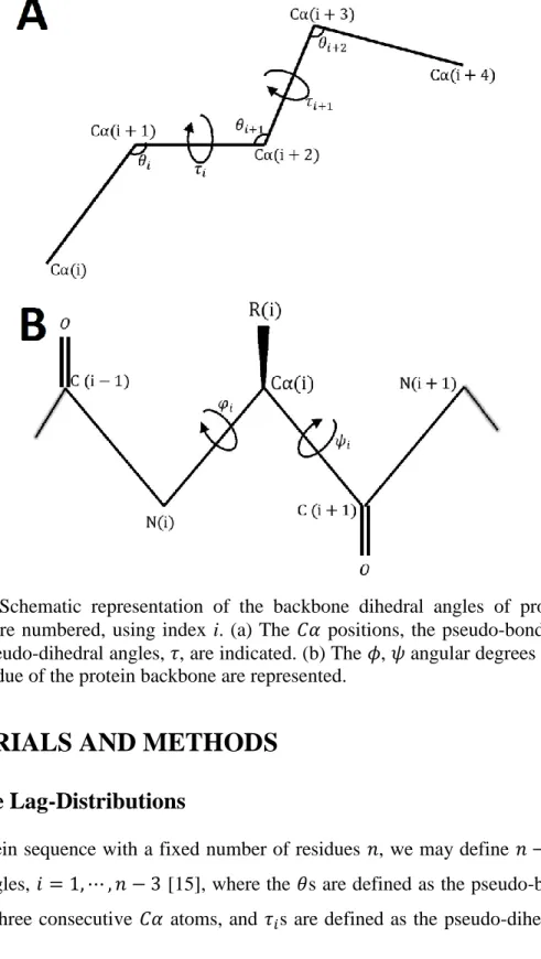
Figure 1: Schematic representation of the backbone dihedral angles of proteins. The positions are numbered, using index i. (a) The 𝐶𝛼 positions, the pseudo-bond angles, 𝜃, and the pseudo-dihedral angles, 𝜏, are indicated. (b) The 𝜙, 𝜓 angular degrees of freedom in one residue of the protein backbone are represented.
MATERIALS AND METHODS
Bivariate Lag-Distributions
For a protein sequence with a fixed number of residues 𝑛, we may define 𝑛 − 3 pairs of
(𝜃𝑖, 𝜏𝑖) angles, 𝑖 = 1, ⋯ , 𝑛 − 3 [15], where the 𝜃s are defined as the pseudo-bond planar angles of three consecutive 𝐶𝛼 atoms, and 𝜏𝑖s are defined as the pseudo-dihedral angles
of four consecutive 𝐶𝛼 atoms, as it is shown in Figure 1a. Similarly, we may obtain 𝑛 − 2
pairs of torsion angles (𝜙𝑖, 𝜓𝑖), 𝑖 = 2, ⋯ , 𝑛 − 1, where the (𝜙, 𝜓) angles directly model the protein backbone structures at the atomic level. The 𝜙 is the torsion angle around the
𝑁 − 𝐶𝛼 bond while the 𝜓 is the torsion angle around the 𝐶𝛼 − 𝐶 bond, as shown in Figure 1b [39].
In general, we introduce the following notation. For a fixed protein, 𝑗, we have 𝑛𝑗
pairs of backbone angles (𝜂𝑖, 𝜁𝑖), where 𝑖 = 1, ⋯ , 𝑛𝑗, and (𝜂, 𝜁)s can be considered as
(𝜃, 𝜏)s, (𝜙, 𝜓)s or any other pairs of angles that construct the protein backbone structure. Following this general framework, it is of great interest in protein conformational sampling to study the joint distribution of the backbone angles,
𝑓(𝜂1, 𝜁1, 𝜂2, 𝜁2, ⋯ , 𝜂𝑛𝑗, 𝜁𝑛𝑗), which is a multivariate distribution with possibly thousands of variables.
The popular Ramachandran plot focuses on bivariate marginal distributions in the angle space and ignores the dependence of the sequence of backbone dihedral angles [14]. To come up with more sophisticated procedures that consider the dependency among the sequences of the dihedral/planar angles, different methods have been proposed in the past decade. Bystroff et al. developed a probabilistic model, HMMSTR, for fragment libraries, which can predict local structures given sequence information [25]. However, the discrete angles used by HMMSTR cause a loss of accuracy. Later, FB5-HMM, a probabilistic model of local protein structures, was proposed by Hamelryck and coworkers to model protein geometry in continuous space [35]. FB5-HMM models protein backbone conformations as a 𝐶𝛼 trace. Therefore, a backbone structure can be uniquely determined and represented by a sequence of (𝜃, 𝜏) angles. FB5-HMM trains an HMM with multiple outputs to learn the joint probability of the amino acid sequence, the secondary structure sequence, and the unit vector sequence, which together determine the backbone structure. The unit vectors are represented by the 5-parameter Fisher-Bingham (FB5) distributions [54]. Protein backbone conformations can then be sampled by using Forward-Backward sampling [59]. Later, Boomsma et al. developed a continuous probabilistic model by considering (𝜙, 𝜓) as the dihedral angles for representing protein backbone structures. A dynamic Bayesian network (DBN) is trained and it captures the joint probabilities of amino acids, secondary structures, (𝜙, 𝜓) angles, and the cis or trans conformation of the
peptide bond. The (𝜙, 𝜓) angle distributions are parameterized by the cosine model [36], which is a Bivariate von Mises distribution. Recently, Lennox and colleagues considered the same problem in a nonparametric Bayesian framework [43, 55]. Their models use Dirichlet processes to obtain mixtures of Bivariate von Mises distributions for modeling the dihedral angles (𝜙, 𝜓) in a fixed position.
We note that the above-mentioned techniques were developed based on the HMM structure, the core of which is the Markov property. The Markov property implies that, for a fixed position in the protein backbone, the conditional distribution of the backbone angles in the current state depends upon a fixed number of previous states. For instance, a first-order HMM property is assumed in [35, 39], whereas a ninth-order HMM property is assumed in [13, 38]. In this paper, we investigate non-fixed lag dependence, i.e., the dependence at various lags. To this end, we let ℓ = 1, … , 𝐿, denote a lag index, where 𝐿 is the maximum number of lags to be considered. For protein 𝑗, the collection of pairs of backbone angles {(𝜂1, 𝜁1+ℓ)⊤, (𝜂
2, 𝜁2+ℓ)⊤, ⋯ , (𝜂𝑛𝑗−ℓ, 𝜁𝑛𝑗)
⊤} can be viewed as a random
draw from the lag-ℓ marginal bivariate density, denoted as 𝑓(ℓ)(𝜂, 𝜁). We propose to use
kernel density estimation [60] with slight modification that considers the angular structure of the data to obtain an estimate of this density. Further details can be found in Supplementary Materials.
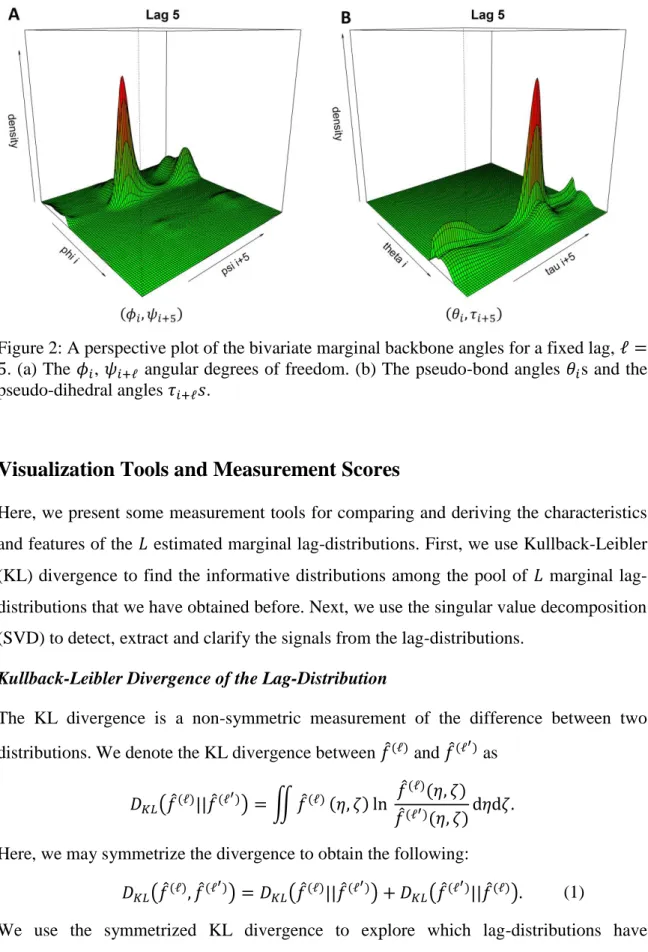
Figure 2 shows the perspective plot for the marginal bivariate kernel density estimates of the backbone angles for a fixed lag, ℓ = 5 (the details of the dataset will be given in the results section). It is known that peaks in lag-zero bivariate distributions, i.e., the (𝜙, 𝜓) distribution (the Ramachandran plot) and the (𝜃, 𝜏) distribution, indicate different secondary structure types [14, 35]. The peaks in lag-distributions also correspond to different secondary structures. For instance, the highest peaks in both Figures 2a and 2b represent alpha-helices. More details can be found in Supplementary Materials.
Figure 2: A perspective plot of the bivariate marginal backbone angles for a fixed lag, ℓ = 5. (a) The 𝜙𝑖, 𝜓𝑖+ℓ angular degrees of freedom. (b) The pseudo-bond angles 𝜃𝑖s and the pseudo-dihedral angles 𝜏𝑖+ℓ𝑠.
Visualization Tools and Measurement Scores
Here, we present some measurement tools for comparing and deriving the characteristics and features of the 𝐿 estimated marginal lag-distributions. First, we use Kullback-Leibler (KL) divergence to find the informative distributions among the pool of 𝐿 marginal lag-distributions that we have obtained before. Next, we use the singular value decomposition (SVD) to detect, extract and clarify the signals from the lag-distributions.
Kullback-Leibler Divergence of the Lag-Distribution
The KL divergence is a non-symmetric measurement of the difference between two distributions. We denote the KL divergence between 𝑓̂(ℓ) and 𝑓̂(ℓ′) as
𝐷𝐾𝐿(𝑓̂(ℓ)||𝑓̂(ℓ ′) ) = ∬ 𝑓̂(ℓ)(𝜂, 𝜁) ln 𝑓̂ (ℓ)(𝜂, 𝜁) 𝑓̂(ℓ′) (𝜂, 𝜁)d𝜂d𝜁.
Here, we may symmetrize the divergence to obtain the following:
𝐷𝐾𝐿(𝑓̂(ℓ), 𝑓̂(ℓ′)) = 𝐷
𝐾𝐿(𝑓̂(ℓ)||𝑓̂(ℓ
′)
) + 𝐷𝐾𝐿(𝑓̂(ℓ′)||𝑓̂(ℓ)). (1)
We use the symmetrized KL divergence to explore which lag-distributions have distinguishing features that are not common across different lags. We expect to see that
the similar lag-distributions have small divergences and the lag-distributions with significant differences in features have higher magnitudes of KL divergence.
Singular Value Decomposition of the Lag-Distributions (LagSVD)
It is possible to obtain an informative and comprehensive measurement for evaluating the
𝐿 estimated marginal bivariate lag-distributions together, in lower dimensions. The intuition is to factorize each bivariate distribution by the sum of 𝑚 multiplicative univariate densities (𝑢1(ℓ), ⋯ , 𝑢𝑚(ℓ)) and (𝑣1(ℓ), ⋯ , 𝑣𝑚(ℓ)) as
𝑓̂(ℓ)(𝜂, 𝜁) = ∑ 𝜎𝑘 𝑚
𝑘=1
𝑢𝑘(ℓ)(𝜂)𝑣𝑘(ℓ)(𝜁) + 𝜖.
Later, we focus on (𝑢𝑘(1), ⋯ , 𝑢𝑘(𝐿)) and (𝑣𝑘(1), ⋯ , 𝑣𝑘(𝐿)) for each 𝑘 (𝑘 = 1, ⋯ , 𝑚), and we track the behavior of the backbone angles across different lags. This idea can be thoroughly justified by introducing the low-rank approximation of the marginal bivariate densities 𝐹̂(ℓ), where 𝐹̂(ℓ) is a 𝑑 × 𝑑 matrix that contains the magnitudes of the joint density (𝑑 is the number of grid points in the directions associated to 𝜂 and 𝜁).
We note that the SVD of 𝐹̂(ℓ) is directly connected to the principal component analysis (PCA) of 𝐹̂(𝑙) and (𝐹̂(ℓ))⊤. Moreover, the dimension reduction tool (SVD or
PCA) that has been used here to reduce the dimensionality of the 𝐿 different bivariate densities is a sensible quantity, and it should not be mistaken by using plain PCA on a sequence of backbone angles, which is definitely not the correct measurement for angular data. More details are given in Supplementary Materials.
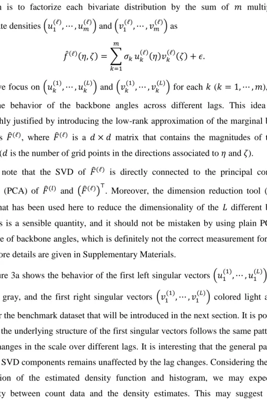
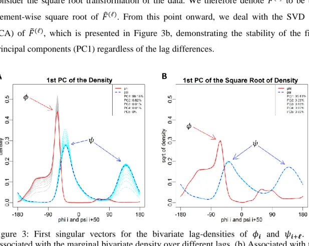
Figure 3a shows the behavior of the first left singular vectors (𝑢1(1), ⋯ , 𝑢1(𝐿)) colored
red and gray, and the first right singular vectors (𝑣1(1), ⋯ , 𝑣1(𝐿)) colored light and dark blue, for the benchmark dataset that will be introduced in the next section. It is possible to see that the underlying structure of the first singular vectors follows the same pattern with some changes in the scale over different lags. It is interesting that the general pattern for the first SVD components remains unaffected by the lag changes. Considering the general association of the estimated density function and histogram, we may expect some similarity between count data and the density estimates. This may suggest that the
changes in the variance could be proportional to the changes in the mean, which is expected from a Poisson family distribution. To overcome this effect, it is common to consider the square root transformation of the data. We therefore denote 𝐹̃(ℓ) to be the element-wise square root of 𝐹̂(ℓ). From this point onward, we deal with the SVD (or PCA) of 𝐹̃(ℓ), which is presented in Figure 3b, demonstrating the stability of the first
principal components (PC1) regardless of the lag differences.
Figure 3: First singular vectors for the bivariate lag-densities of 𝜙𝒊 and 𝜓𝒊+𝓵. (a) Associated with the marginal bivariate density over different lags. (b) Associated with the element-wise square root of the marginal bivariate density over different lags.
RESULTS
In this section, we start by presenting some findings about the behavior of the marginal lag-distributions of the backbone angles of different lags, and subsequently we discuss how we may use these tractable behaviors to develop an assessment tool for evaluating different conformational sampling methods for proteins. Also, we use the CASP9 datasets to demonstrate the applicability of using the marginal lag-distributions over different lags for quality assessment of general protein prediction methods in terms of preserving the angular structure.
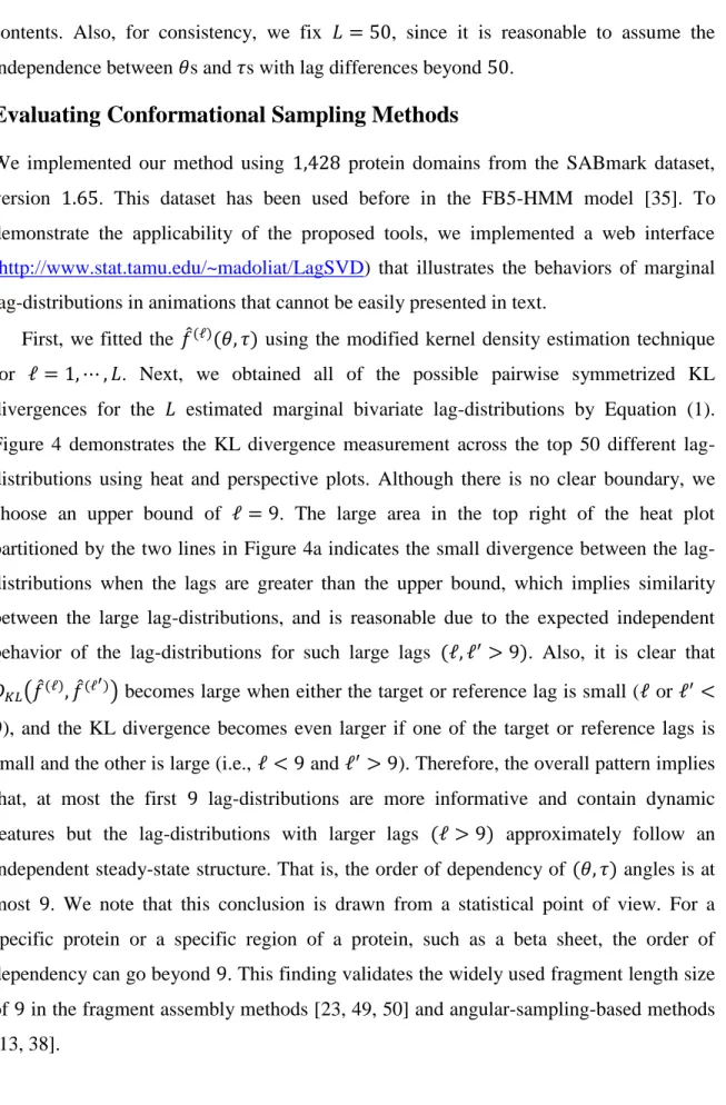
We focus on the (𝜃, 𝜏) description in this section, but similar results can be obtained for the representation of the dihedral angles (𝜙, 𝜓), which we skip for brevity of the
contents. Also, for consistency, we fix 𝐿 = 50, since it is reasonable to assume the independence between 𝜃s and 𝜏s with lag differences beyond 50.
Evaluating Conformational Sampling Methods
We implemented our method using 1,428 protein domains from the SABmark dataset, version 1.65. This dataset has been used before in the FB5-HMM model [35]. To demonstrate the applicability of the proposed tools, we implemented a web interface (http://www.stat.tamu.edu/~madoliat/LagSVD) that illustrates the behaviors of marginal lag-distributions in animations that cannot be easily presented in text.
First, we fitted the 𝑓̂(ℓ)(𝜃, 𝜏) using the modified kernel density estimation technique
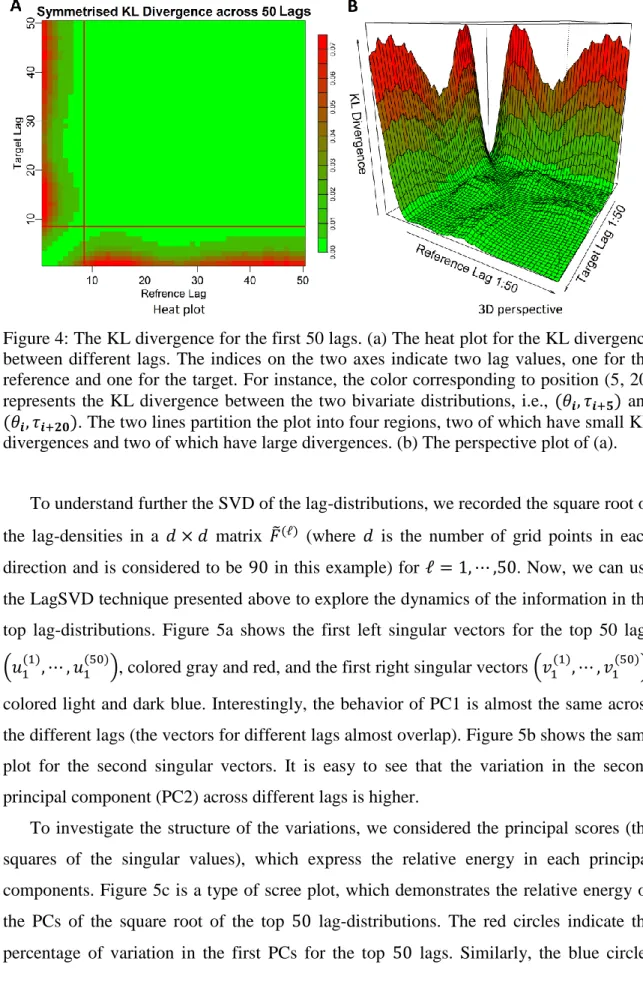
for ℓ = 1, ⋯ , 𝐿. Next, we obtained all of the possible pairwise symmetrized KL divergences for the 𝐿 estimated marginal bivariate lag-distributions by Equation (1). Figure 4 demonstrates the KL divergence measurement across the top 50 different lag-distributions using heat and perspective plots. Although there is no clear boundary, we choose an upper bound of ℓ = 9. The large area in the top right of the heat plot partitioned by the two lines in Figure 4a indicates the small divergence between the lag-distributions when the lags are greater than the upper bound, which implies similarity between the large lag-distributions, and is reasonable due to the expected independent behavior of the lag-distributions for such large lags (ℓ, ℓ′ > 9). Also, it is clear that 𝐷𝐾𝐿(𝑓̂(ℓ), 𝑓̂(ℓ′)) becomes large when either the target or reference lag is small (ℓ or ℓ′ < 9), and the KL divergence becomes even larger if one of the target or reference lags is small and the other is large (i.e., ℓ < 9 and ℓ′> 9). Therefore, the overall pattern implies that, at most the first 9 lag-distributions are more informative and contain dynamic features but the lag-distributions with larger lags (ℓ > 9) approximately follow an independent steady-state structure. That is, the order of dependency of (𝜃, 𝜏) angles is at most 9. We note that this conclusion is drawn from a statistical point of view. For a specific protein or a specific region of a protein, such as a beta sheet, the order of dependency can go beyond 9. This finding validates the widely used fragment length size of 9 in the fragment assembly methods [23, 49, 50] and angular-sampling-based methods [13, 38].
Figure 4: The KL divergence for the first 50 lags. (a) The heat plot for the KL divergence between different lags. The indices on the two axes indicate two lag values, one for the reference and one for the target. For instance, the color corresponding to position (5, 20) represents the KL divergence between the two bivariate distributions, i.e., (𝜃𝒊, 𝜏𝒊+𝟓) and
(𝜃𝒊, 𝜏𝒊+𝟐𝟎). The two lines partition the plot into four regions, two of which have small KL divergences and two of which have large divergences. (b) The perspective plot of (a).
To understand further the SVD of the lag-distributions, we recorded the square root of the lag-densities in a 𝑑 × 𝑑 matrix 𝐹̃(ℓ) (where 𝑑 is the number of grid points in each
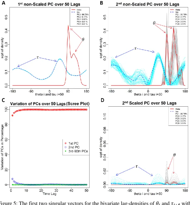
direction and is considered to be 90 in this example) for ℓ = 1, ⋯ ,50. Now, we can use the LagSVD technique presented above to explore the dynamics of the information in the top lag-distributions. Figure 5a shows the first left singular vectors for the top 50 lags
(𝑢1(1), ⋯ , 𝑢1(50)), colored gray and red, and the first right singular vectors (𝑣1(1), ⋯ , 𝑣1(50)), colored light and dark blue. Interestingly, the behavior of PC1 is almost the same across the different lags (the vectors for different lags almost overlap). Figure 5b shows the same plot for the second singular vectors. It is easy to see that the variation in the second principal component (PC2) across different lags is higher.
To investigate the structure of the variations, we considered the principal scores (the squares of the singular values), which express the relative energy in each principal components. Figure 5c is a type of scree plot, which demonstrates the relative energy of the PCs of the square root of the top 50 lag-distributions. The red circles indicate the percentage of variation in the first PCs for the top 50 lags. Similarly, the blue circles
indicate the percentage of variation in the second PCs, and the green circles indicate the percentage of variation in the remaining PCs (see Supplementary Materials for more details). Obviously, beyond the second PCs, the cumulative information in the remaining PCs is negligible. Moreover, the information in the second PCs, which seems to be related to the dependency structure, decreases with the increment of the lags, and it almost vanishes beyond the 9th lag. This further confirms that, statistically, little information can
be gained beyond a dependency order of nine. Next, we integrated the energy associated with each PC by multiplying the singular vectors with the associated singular values to obtain scaled singular vectors. The pattern for the scaled PC1 is very similar to the pattern in Figure 5a, which we do not discuss for brevity. The scaled PC2 is shown in Figure 5d, however. It indicated how smoothly the structure of the dependency vanishes in the first 9
lags. The animations presented at http://www.stat.tamu.edu/∼madoliat/LagSVD are helpful in depicting the associated behaviors.
We further came up with some measurements for model assessment based on symmetrized KL divergences. For demonstration purposes, we focused on two commonly used HMM models and one baseline method. In all three methods, an HMM is considered to have three observations, the joint probability of the amino acid sequence, the secondary structure sequence, and the quantity of interest in this paper, which is the distribution of the dihedral/planar angles in the backbone structure. The three methods are (a) FB5-HMM: This parametric protein conformation sampling technique was introduced in [35]. Since 0 < 𝜃 < 𝜋 is a planar angle and −𝜋 < 𝜏 < 𝜋 is a dihedral angle, they used the Fisher-Bingham distribution with 5 parameters (FB5), which is defined on a sphere for modeling (𝜃, 𝜏) angles. (b) BVM-HMM: Boomsma et al. used the Bivariate von Mises (BVM) distribution to model dihedral angles −𝜋 < 𝜙, 𝜓 < 𝜋 on a torus [39]. Here, we adopted their HMM model for (𝜃, 𝜏) representation. Clearly, the density of (𝜃, 𝜏) will be zero on half of the torus where −𝜋 < 𝜃 < 0, but this will not be problematic for
Figure 5: The first two singular vectors for the bivariate lag-densities of 𝜃𝒊 and 𝜏𝒊+𝓵 with a scree plot. (a) Non-scaled first singular vectors for different lags. The vectors almost overlap, suggesting that the first lag is very conserved. (b) Non-scaled second singular vectors for different lags. (c) A scree plot of the relative energy of the SVD components corresponding to the square root of the top 50 lag-distributions. (d) Scaled second singular vectors with respect to the associated singular values.
interpretation. (c) BVN-HMM: Although it seems not reasonable to use a Bivariate normal (BVN) for modeling backbone angles because BVN does not consider the correct boundary conditions, we used it as a baseline method to check its performance against the other two commonly used models.
For the training and simulation purposes we used Mocapy++ [42], which is a freely available toolkit for parameter learning in dynamic Bayesian networks (DBN). It supports a wide range of DBN architectures and probability distributions, including distributions from directional statistics. In training the three HMM models, we considered four different numbers of hidden nodes, 𝐻 = {25,50,75,100}, and five different initial seeds. We therefore ended up with 60 trained models, and we simulated 100 protein structures for each trained model, each with 100 amino acids.
The idea was to train each model (or use the trained models provided in the corresponding works), sample a set of protein structures accordingly, and then compare the statistical characteristics of the sampled set with the training set at different lags. For each simulation, (𝑚 = 1, ⋯ ,60), and lag, ℓ (ℓ = 1, ⋯ ,50), we therefore considered the symmetrized KL divergence (SKLD) as
SKLD𝑚(ℓ) = 𝐷𝐾𝐿(𝑓̂𝑟(ℓ), 𝑓̂𝑚(ℓ)),
where 𝑓̂𝑟(ℓ) is the nonparametric estimation of the marginal bivariate lag-distribution at lag
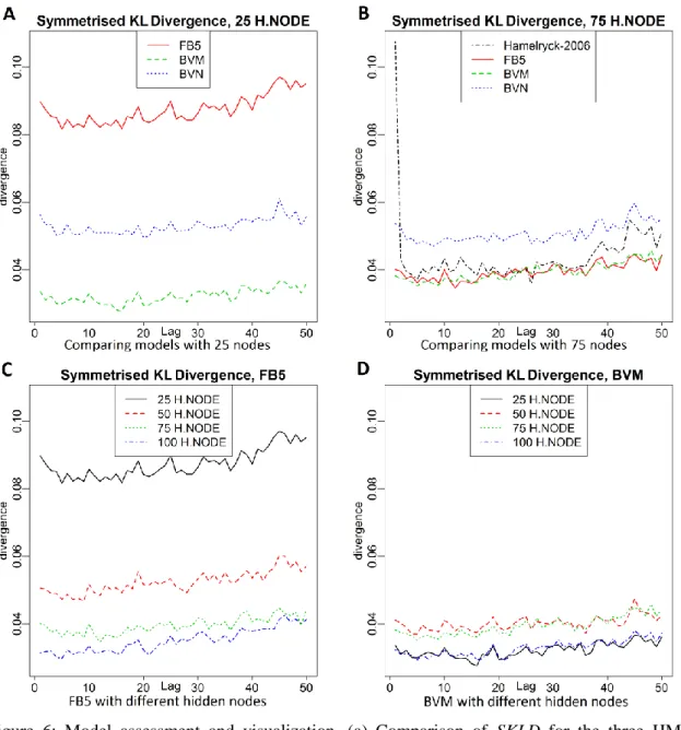
ℓ for the benchmark dataset, and 𝑓̂𝑚(ℓ) is the same quantity for the simulated data, 𝑚. First, we considered three bivariate distributions (FB5, BVN and BVM) that have been used to model dihedral/planar angles with 25 hidden nodes in the HMM, and we averaged over the initial seeds. Figure 6a shows the differences in SKLD for these three models at different lags. Surprisingly, the BVN obtained a better fit compared with the FB5, a circular analog of the BVN, in terms of KL divergence. On the other hand, BVM seemed to be the best choice for modeling the backbone angles.
Figure 6b compares the three HMM models (FB5, BVN and BVM) with 75 hidden nodes plus the Hamelryck results (FB5-HMM) that is given in [35]. The closeness in performance of BVM and FB5 models, which outperform BVN, is expected. Although the results in [35] should be similar to those of FB5, its SKLD is larger than that of the FB5 model, especially for the first 3 lags. A possible explanation could be the technical improvements in the Mocapy++ software [42] in recent years.
Next, we focused on the simulation runs obtained from the FB5 fits, averaged over the initial seeds. Figure 6c compares the SKLD among four numbers of hidden nodes (𝐻 = 25,50,75,100), in the structure of the FB5-HMM model. The improvement in the performance of the FB5-HMM model by increasing the number of hidden nodes from 25
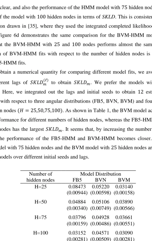
to 75 is clear, and also the performance of the HMM model with 75 hidden nodes is close to that of the model with 100 hidden nodes in terms of SKLD. This is consistent with the conclusion drawn in [35], where they used the integrated completed likelihood criterion (ICL). Figure 6d demonstrates the same comparison for the BVM-HMM models. It is clear that the BVM-HMM with 25 and 100 nodes performs almost the same, and the variation of BVM-HMM fits with respect to the number of hidden nodes is much less than FB5-HMM fits.
To obtain a numerical quantity for comparing different model fits, we averaged out the different lags of 𝑆𝐾𝐿𝐷𝑚(ℓ) to obtain 𝑆𝐾𝐿𝐷𝑚. We prefer the models with smaller
𝑆𝐾𝐿𝐷𝑚. Here, we integrated out the lags and initial seeds to obtain 12 estimates for
𝑆𝐾𝐿𝐷𝑚 with respect to three angular distributions (FB5, BVN, BVM) and four numbers
of hidden nodes (𝐻 = 25,50,75,100). As shown in Table 1, the BVM model achieves the best performance for different numbers of hidden nodes, whereas the FB5-HMM with 25
hidden nodes has the largest 𝑆𝐾𝐿𝐷𝑚. It seems that, by increasing the number of hidden
nodes, the performance of the FB5-HMM and BVM-HMM becomes closer. Also, the FB5 model with 75 hidden nodes and the BVM model with 25 hidden nodes are the most robust models over different initial seeds and lags.
Number of Model Distribution hidden nodes FB5 BVN BVM H=25 0.08473 0.05220 0.03140 (0.00944) (0.00598) (0.00158) H=50 0.04884 0.05106 0.03890 (0.00340) (0.00749) (0.00566) H=75 0.03796 0.04928 0.03661 (0.00159) (0.00486) (0.00551) H=100 0.03152 0.04571 0.03090 (0.00281) (0.00509) (0.00281)
Table 1: Comparisons of SKLD between the HMM models with FB5, BVN, and BVM angular distributions for different numbers of hidden nodes. The values within the parenthesis are the associated standard errors.
Figure 6: Model assessment and visualization. (a) Comparison of SKLD for the three HMM models, i.e., Bivariate Normal, FB5 and Bivariate von Mises with 25 hidden nodes. (b) Comparison of SKLD for the three HMM models and the FB5-HMM fit of [35] with 75 hidden nodes. (c) Comparison of SKLD for the FB5 model with different numbers of hidden nodes. (d) Comparison of SKLD for the BVM model with different numbers of hidden nodes.
Quality Assessment for General Structure Prediction Methods
The marginal lag-distributions of angles can also be straightforwardly applied to extract information from any given set of protein structures, and thus can be used as a quality assessment tool for any protein structure prediction method. To explore this technique in general, we considered 115 target proteins presented in the recent CASP9, which were
mostly predicted by the major protein structure prediction servers. Similar to the previous experiments, we obtained the marginal lag-distributions 𝑓̂(ℓ)(𝜃, 𝜏) for the native structure
pool that was specified in the CASP9 website, and four well-performed servers “HHpredA” [34, 61], “RaptorX” [62], “Rosetta Server” [23, 49, 50] and “Zhang Server” [40, 51, 52].
We used the 𝑆𝐾𝐿𝐷𝑚ℓ measurement to assess the quality of predictions for each of the
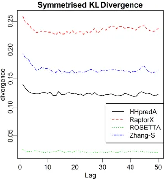
four servers by comparing to the native structure pool of the 115 target proteins. Figure 7 compares the 𝑆𝐾𝐿𝐷𝑚ℓ across the first 50 lags of bivariate-marginal lag-distributions for each of the four servers. As shown in the figure, “Rosetta Server” outperforms all other servers over all the lags. This is expected because “Rosetta Server” is the only method among the four that directly models protein structures in angular space. When assessed by coordinate-based measurements, such as RMSD, TM-score and the GDT score, “Zhang Server” was ranked the best among the four [6]. The different assessment results imply that although the “Rosetta Server” predicted angles more accurately, it lost accuracy in building the 3D structural models because of the use of the ideal values of bond length and bond angles.
Figure 7: Model assessment and visualization for comparing the SKLD among four well-performed servers, “HHpredA”, “RaptorX”, “Rosetta Server” and “Zhang Server”, versus the native structure pool.
DISCUSSION
A common belief is that angular sampling methods could be considered as potential aids in solving the protein structure prediction problem, especially in discovering the new-fold protein targets. Different modeling techniques for established angular sampling methods have therefore been proposed in the literature over the past decade, but there is no systematic method to evaluate the accuracy of the proposed models. Marginal bivariate lag-distributions can be used as an assessment measure for protein conformational sampling methods. Furthermore, LagSVD can be straightforwardly applied to provide a statistical evaluation of any protein structure prediction method. Traditional quality assessment methods have bottlenecks. For example, coordinate-based measurements can be biased by the use of expected bond and angle constants, and single structure-based measurements can also be biased by special cases. By directly and systematically measuring the structure prediction methods in angular space, LagSVD can provide the research community with an alternative measure and perspective.
Our findings on a benchmark protein structure dataset show that little information is contained beyond a dependency order of nine. This suggests that future graphical models for angular sampling methods, such as hidden Markov models and conditional random fields, need not use very large window sizes, even if inference algorithms are available for such high-order models. Long-range contacts, which are known to play essential roles in protein folding, could be modeled in a specific protein-dependent manner.
We found that the FB5 distribution did not perform as expected in modeling (𝜃, 𝜏) angles. In fact, the FB5-HMM with a small number of hidden nodes performed worse than the bivariate normal distribution, which does not take the circular nature of angles into consideration. The Bivariate von Mises models performed the best among the three angular distribution models we considered for (𝜃, 𝜏) angles.
SUPPLEMENTARY DATA
Supplementary materials are available online athttp://bib.oxfordjournals.org.
Also, to illustrate the results and provide service to the community, we have developed a webserver at http://www.stat.tamu.edu/∼madoliat/LagSVD.
Acknowledgments
The authors would like to thank Anna Tramontano and three reviewers for the thoughtful comments that helped us to improve the manuscript. We thank Virginia Unkefer for the editorial work.
FUNDING
This work was supported by grants from NCI (CA57030), NSF (DMS-0907170, DMS- 1007618), and Award Numbers KUS-CI-016-04 and GRP-CF-2011-19-P-Gao-Huang, made by King Abdullah University of Science and Technology (KAUST).
References
1. Moult J, Fidelis K, Zemla A, et al. Critical assessment of methods of protein structure prediction (CASP)–round V. Proteins 2003;53(Suppl 6):334–9.
2. Moult J. A decade of CASP: progress, bottlenecks and prognosis in protein structure prediction. Curr
Opin Struct Biol 2005;15:285–9.
3. Moult J, Fidelis K, Rost B, et al. Critical assessment of methods of protein structure prediction (CASP)–round VI. Proteins 2005;61(Suppl 7):3–7.
Key Points
• Marginal bivariate lag-distributions can be used to explore the dependence structure of dihedral/planar angles across different lags. They can also be used to assess and compare the accuracy of different model fits.
• LagSVD is useful to extract information from the marginal bivariate lag-distributions of dihedral/planar angles and visualize this information in the lower dimensions.
• Although intuition suggests that the higher-order models of a fragment-based method or an angular-sampling-based technique should achieve better performance, we have seen that the dependency structure of dihedral/planar angles vanishes for the lags beyond nine in the real protein structures. Therefore, use of any higher-order model seems to be unnecessary. • We have observed that the commonly used FB5 distribution, which has been used for modeling
the dihedral/planar angular structure, is not necessarily the best option as was expected from a theoretical point of view.
• BVM-HMM with a small number of hidden nodes performs quite well in modeling dihedral/planar angles.
4. Moult J, Fidelis K, Kryshtafovych A, et al. Critical assessment of methods of protein structure prediction–round VII. Proteins 2007;69(Suppl 8):3–9.
5. Moult J, Fidelis K, Kryshtafovych A, et al. Critical assessment of methods of protein structure prediction–round VIII. Proteins 2009;77(Suppl 9):1–4.
6. Moult J, Fidelis K, Kryshtafovych A, et al. Critical assessment of methods of protein structure prediction (CASP)–round IX. Proteins 2011;79(Suppl 10):1–5.
7. Xu Y, Xu D, Liang J. Computational methods for protein structure prediction and modeling. Volume 1, New York: Springer, 2007.
8. Xu Y, Xu D, Liang J. Computational methods for protein structure prediction and modeling. Volume 2, New York: Springer, 2007.
9. Jauch R, Yeo HC, Kolatkar PR, et al. Assessment of CASP7 structure predictions for template free targets. Proteins 2007;69(Suppl 8):57–67.
10. Dill KA, Ozkan SB, Weikl TR, et al. The protein folding problem: when will it be solved? Curr Opin
Struct Biol 2007;17:342-6
11. Berman HM, Westbrook J, Feng Z, et al. The protein data bank. Nucleic Acids Res 2000;28:235–42. 12. Anfinsen CB. Principles that govern the folding of protein chains. Science 1973;181:223–30.
13. Zhao F, Li S, Sterner BW, et al. Discriminative learning for protein conformation sampling. Proteins
2008;73:228–40.
14. Ramachandran GN, Ramakrishnan C, Sasisekharan V. Stereochemistry of polypeptide chain configurations. J Mol Biol 1963;7:95–9.
15. Levitt M. A simplified representation of protein conformations for rapid simulation of protein folding.
J Mol Biol 1976;104:59–107.
16. Holm L, Sander C. Database algorithm for generating protein backbone and side-chain co-ordinates from a C alpha trace application to model building and detection of co-ordinate errors. J Mol Biol
1991;218:183–94.
17. Maupetit J, Gautier R, Tufféry P. SABBAC: online Structural Alphabet-based protein BackBone reconstruction from Alpha-Carbon trace. Nucleic Acids Res 2006;34:W147-51.
18. Gront D, Kmiecik S, Kolinski A. Backbone building from quadrilaterals: a fast and accurate algorithm for protein backbone reconstruction from alpha carbon coordinates. J Comput Chem 2007;28:1593–7. 19. Claessens M, Van Cutsem E, Lasters I, et al. Modelling the polypeptide backbone with ’spare parts’
from known protein structures. Protein Eng 1989;2:335–45.
20. Unger R, Harel D, Wherland S, et al. A 3D building blocks approach to analyzing and predicting structure of proteins. Proteins 1989;5:355–73.
21. Levitt M. Accurate modeling of protein conformation by automatic segment matching. J Mol Biol
1992;226:507–33.
22. Wendoloski JJ, Salemme FR. PROBIT: a statistical approach to modeling proteins from partial coordinate data using substructure libraries. J Mol Graphics 1992;10:124–6.
23. Simons KT, Kooperberg C, Huang E, et al. Assembly of protein tertiary structures from fragments with similar local sequences using simulated annealing and Bayesian scoring functions. J Mol Biol
1997;268:209–25.
24. Xia Y, Huang ES, Levitt M, et al. Ab initio construction of protein tertiary structures using a hierarchical approach. J Mol Biol 2000;300:171–85.
25. Bystroff C, Thorsson V, Baker D. HMMSTR: a hidden Markov model for local sequence-structure correlations in proteins. J Mol Biol 2000;301:173–90.
26. Feldman HJ, Hogue CW. A fast method to sample real protein conformational space. Proteins
2000;39:112–31.
27. Oldfield TJ. A number of real-space torsion-angle refinement techniques for proteins, nucleic acids, ligands and solvent. Acta Crystallogr D Biol Crystallogr 2001;57:82–94.
28. Fain B, Levitt M. A novel method for sampling alpha-helical protein backbones. J Mol Biol
2001;305:191-201.
29. Kolodny R, Koehl P, Guibas L, et al. Small libraries of protein fragments model native protein structures accurately. J Mol Biol 2002;323:297–307.
30. Gong H, Fleming PJ, Rose GD. Building native protein conformation from highly approximate backbone torsion angles. P Natl Acad Sci 2005;102:16227–32.
31. Bradley P, Misura KM, Baker D. Toward high-resolution de novo structure prediction for small proteins. Science 2005;309:1868–71.
32. Tuffery P, Derreumaux P. Dependency between consecutive local conformations helps assemble protein structures from secondary structures using Go potential and greedy algorithm. Proteins
2005;61:732–40.
33. Zhang Y, Skolnick J. The protein structure prediction problem could be solved using the current PDB library. P Natl Acad Sci 2005;102:1029–34.
34. Söding J. Protein homology detection by HMM-HMM comparison. Bioinformatics 2005;21:951–60. 35. Hamelryck T, Kent JT, Krogh A. Sampling realistic protein conformations using local structural bias.
PLoS Comput Biol 2006;2:e131.
36. Mardia KV, Taylor CC, Subramaniam GK. Protein bioinformatics and mixtures of bivariate von Mises distributions for angular data. Biometrics 2007;63:505–12.
37. Biegert A, Sцding J. De novo identification of highly diverged protein repeats by probabilistic consistency. Bioinformatics 2008;24:807–14.
38. Li SC, Bu D, Xu J, et al. Fragment-HMM: a new approach to protein structure prediction. Protein Sci
2008;17:1925–34.
39. Boomsma W, Mardia KV, Taylor CC, et al. A generative, probabilistic model of local protein structure. P Natl Acad Sci 2008;105:8932–37.
41. Faraggi E, Yang Y, Zhang S, et al. Predicting continuous local structure and the effect of its substitution for secondary structure in fragment-free protein structure prediction. Structure
2009;17:1515–27.
42. Paluszewski M, Hamelryck T. Mocapy++ – A toolkit for inference and learning in dynamic Bayesian networks. BMC Bioinformatics 2010;11:126.
43. Lennox KP, Dahl DB, Vannucci M, et al. Dirichlet process mixture of hidden Markov models for protein structure prediction. Ann Appl Stat 2010;4:916–42.
44. Zhao F, Peng J, Debartolo J, et al. A probabilistic and continuous model of protein conformational space for template-free modeling. J Comput Biol 2010;17:783–98.
45. Zhou Y, Duan Y, YangY, et al. Trends in template/fragment-free protein structure prediction. Theor
Chem Acc 2011;128:3–16.
46. Hu Y, Dong X, Wu A, et al. Incorporation of local structural preference potential improves fold recognition. PLoS One 2011;6:e17215.
47. Jones TA, Thirup S. Using known substructures in protein model building and crystallography. EMBO J 1986;5:819–22.
48. Simon I, Glasser L, Scheraga HA. Calculation of protein conformation as an assembly of stable overlapping segments: application to bovine pancreatic trypsin inhibitor. P Natl Acad Sci
1991;88:3661–5.
49. Chivian D, Kim DE, Malmstrцm L, et al. Automated prediction of CASP-5 structures using the Robetta server. Proteins 2003;53(Suppl 6):524–33.
50. Raman S, Vernon R, Thompson J, et al. Structure prediction for CASP8 with all-atom refinement using Rosetta. Proteins 2009;77(Suppl 9):89–99.
51. Roy A, Kucukural A, Zhang Y. I-TASSER: a unified platform for automated protein structure and function prediction. Nat Protoc 2010;5:725–38.
52. Roy A, Xu D, Poisson J, et al. A protocol for computer-based protein structure and function prediction. JoVE 2011;57:e3259.
53. Camproux AC, Tuffery P, Chevrolat JP, et al. Hidden Markov model approach for identifying the modular framework of the protein backbone. Protein Eng 1999;12:1063–73.
54. Kent JT. The Fisher-Bingham distribution on the sphere. J R Statist Soc B 1982;44:71–80.
55. Lennox KP, Dahl DB, Vannucci M, et al. Density estimation for protein conformation angles using a bivariate von Mises distribution and Bayesian nonparametrics. J Amer Statist Assoc 2009;104:586–96. 56. Cozzetto D, Kryshtafovych A, Fidelis K, et al. Evaluation of template-based models in CASP8 with
standard measures. Proteins 2009;77(Suppl 9):18–28.
57. Zhang Y, Skolnick J. Scoring function for automated assessment of protein structure template quality.
Proteins 2004;57:702–10.
58. Zemla A, Venclovas C, Moult J, et al. Processing and analysis of CASP3 protein structure predictions.
59. Cawley SL, Pachter L. HMM sampling and applications to gene finding and alternative splicing.
Bioinformatics 2003;19(Suppl 2):ii36-41.
60. Wand M, Jones M. Kernel smoothing, Monographs on statistics and applied probability. New York: Chapman & Hall, 1995.
61. Söding J, Biegert A, Lupas AN. The HHpred interactive server for protein homology detection and structure prediction. Nucleic Acids Res 2005;33:W244–8.
62. Peng J, Xu J. RaptorX: exploiting structure information for protein alignment by statistical inference.
Proteins 2011;79(Suppl 10):161–71.
63. Stewart GW. On the early history of the singular value decomposition. SIAM Review 1993;21:951–60. 64. Venables WN, Ripley BD. Modern Applied Statistics with S. New York: Springer, 2002.