Relevant Accessible Sensitivity Analysis for Clinical Trials with Missing Data

(1)

Cro, S (2017) Relevant Accessible Sensitivity Analysis for Clinical Trials with Missing Data. PhD thesis, London School of Hygiene & Tropical Medicine. DOI: https://doi.org/10.17037/PUBS.03817571

Downloaded from: http://researchonline.lshtm.ac.uk/3817571/

DOI:10.17037/PUBS.03817571

Usage Guidelines

Please refer to usage guidelines at http://researchonline.lshtm.ac.uk/policies.html or alterna-tively [email protected].

(2)

Relevant Accessible Sensitivity Analysis

for Clinical Trials with Missing Data

Suzie Cro

Thesis submitted in accordance with the requirements for the degree

of Doctor of Philosophy of the University of London

January 2017

Department of Medical Statistics

Faculty of Epidemiology and Population Health

London School of Hygiene and Tropical Medicine

Funded by the MRC Clinical Trials Unit,

at University College London

(3)

Declaration

I, Suzie Cro, confirm that the work presented in this thesis is my own.

Where information has been derived from other sources, I confirm that this has been indicated in the thesis.

(4)

Abstract

The statistical analysis of longitudinal randomised controlled trials is frequently complicated by the occurrence of protocol deviations which result in incomplete datasets for analysis. However analysis is approached, an unverifiable assumption about the distribution of the unobserved post-deviation data must be made. In such circumstances it is consequently important to assess the robustness of the primary analysis of the trial to different credible assumptions about the distribution of the missing data.

Reference based multiple imputation procedures have been proposed for contextually relevant sensitivity analysis of longitudinal trials. Differences between the mean and variance of observed and missing data are specified with qualitative reference to trial arms and multiple imputation is used for estimation and inference. The primary analysis model is retained in the sensitivity analysis to assess the impact of alternative sampling behaviour on the original planned analysis. Rubin’s rules are used to combine the treatment effect and variance estimates across imputed datasets, however it is unclear precisely what an appropriate measure of variance is in this setting and how Rubin’s variance formula relates to this.

We begin by defining a lower bound for variance estimation in the reference based settings as the variance estimate we would obtain were we able to observe the deviation data under the postulated post-deviation data assumption. We show Rubin’s variance estimate always exceeds this and moreover it approximately preserves the loss of information in the primary analysis. We also explore Rubin’s variance estimate in theδ-adjusted sensitivity analysis setting and show that Rubin’s variance formula preserves the loss of information in this context.

Alongside, we develop a new Stata command “mimix” for implementation of reference based sensi-tivity analyses. We illustrate the relevance and accessibility of the proposed methods of sensisensi-tivity analysis using data from a chronic asthma trial and a study of peer review.

(5)

7.3 The ‘δ-method’ . . . 226 7.4 Generalisability . . . 227 7.5 Information anchoring . . . 230 7.6 Future work . . . 231 7.7 Concluding remarks . . . 233 Appendices 234 A Exploratory simulation study details 234 B Reference based computations; baseline and single follow-up 235 B.1 The design based variance estimator when post-deviation data is observed . . . 235

(8)

B.2 The design based variance estimator when post-deviation data is unobserved;

maximum likelihood analysis result . . . 237

B.3 Reference based imputation models . . . 239

B.4 Imputation calculations . . . 244

B.4.1 MAR imputation calculations . . . 244

B.4.2 CR imputation calculations . . . 247

B.4.3 J2R imputation calculations . . . 251

B.4.4 CIR imputation calculations . . . 254

B.4.5 LMCF imputation calculations . . . 257

C Additional results from baseline and single follow-up simulation studies 262 D Reference based computations; longitudinal setting 273 D.1 The design based variance estimator when post-deviation data is observed . . . 273

D.1.1 Last measured variable subject to non-response . . . 273

D.1.2 Monotone non-response . . . 275

E Longitudinal simulation studies 277 E.1 Imposed missing data patterns . . . 277

E.2 Additional results . . . 278

F The ‘δ-method’ computations 281 F.1 The design based variance estimator when post-deviation data is observed; baseline and single follow-up . . . 281

F.2 The design based variance estimator when post-deviation data is unobserved; imputation calculations . . . 282

F.3 The design based variance estimator when post-deviation data is observed; longitudinal setting . . . 284

(9)

List of Figures

1.1 Illustration of the ‘δ-method’ . . . 38

1.2 Illustration of jump to reference imputation . . . 40

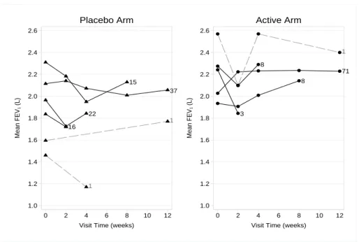
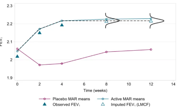
1.3 Asthma trial: observed mean FEV1and deviation profile by treatment arm . . . . 42

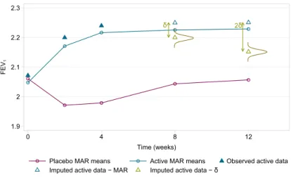
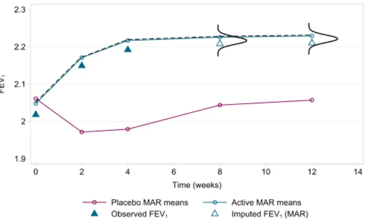
2.1 MAR mean profiles in the asthma RCT . . . 46

2.2 Drawing imputed data under MAR in the asthma RCT . . . 46

2.3 Drawing imputed data under CIR in the asthma RCT . . . 48

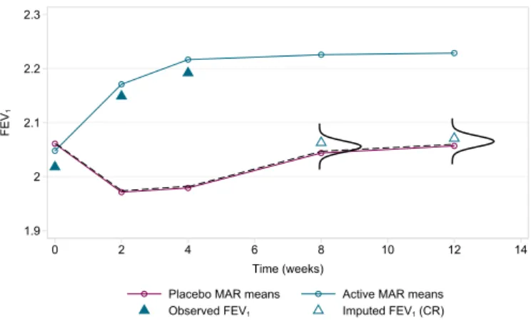
2.4 Drawing imputed data under CR in the asthma RCT . . . 48

2.5 Drawing imputed data under LMCF in the asthma RCT . . . 49

2.6 Rubin’s variance vs. conventional long-run sampling variance vs. lower bound for MAR, LMCF and CR . . . 63

2.7 Rubin’s variance vs. conventional long-run sampling variance vs. lower bound for CIR and J2R . . . 63

3.1 Rubin’s variance estimator vs. information anchored variance . . . 95

3.2 Rubin’s variance estimator vs. information anchored variance with n=100 per arm 96 3.3 Rubin’s variance estimator vs. information anchored variance with n=1000 per arm 96 3.4 Rubin’s variance estimator vs. information anchored variance with a low covariance structure . . . 97

3.5 Rubin’s variance estimator vs. information anchored variance with a high covariance structure . . . 98

3.6 Rubin’s baseline adjusted variance estimator vs. the baseline adjusted information anchored variance . . . 117

3.7 Rubin’s baseline adjusted variance estimator vs. the baseline adjusted information anchored variance with n=100 per arm . . . 118

3.8 Rubin’s baseline adjusted variance estimator vs. the baseline adjusted information anchored variance with n=1000 per arm . . . 118

3.9 Rubin’s baseline adjusted variance estimator vs. the baseline adjusted information anchored variance with a low covariance structure . . . 119

3.10 Rubin’s baseline adjusted variance estimator vs. the baseline adjusted information anchored variance with a high correlation structure . . . 119

4.1 Information anchored variance vs. RHS1 and RHS2 . . . 132

4.2 CR MI with implementation for improved information anchoring . . . 136

4.3 J2R MI with implementation for improved information anchoring . . . 136

4.4 CIR MI with implementation for improved information anchoring . . . 137

4.5 Rubin’s variance estimator vs. information anchored variance in the longitudinal setting . . . 163

(10)

4.6 Rubin’s variance estimator vs. information anchored variance in the longitudinal

setting with n=100 per arm . . . 164

4.7 Rubin’s variance estimator vs. information anchored variance in the longitudinal setting with n=1000 per arm . . . 164

4.8 Rubin’s variance estimator vs. information anchored variance in the longitudinal setting with a low covariance structure . . . 165

4.9 Rubin’s variance estimator vs. information preserving variance in the longitudinal setting with a high covariance structure . . . 165

4.10 Rubin’s variance estimator vs. information anchored variance in the longitudinal setting with deviation in both arms . . . 167

4.11 Rubin’s variance estimator vs. information anchored variance in the longitudinal setting with deviation in both arms; deviation active = 2x deviation placebo . . . 167

5.1 Rubin’s +δadjusted variance estimator vs. information anchored variance . . . 188

5.2 Rubin’s−δadjusted variance estimator vs. information anchored variance . . . 188

5.3 Rubin’s −δ adjusted variance estimator vs. information anchored variance with σ_δ2= 0.012 . . . 189

5.4 Rubin’s −δ adjusted variance estimator vs. information anchored variance with σ_δ2= 0.052 . . . 190

5.5 Rubin’s +δ adjusted variance estimator vs. information anchored variance in the longitudinal setting . . . 199

5.6 Rubin’s −δ adjusted variance estimator vs. information anchored variance in the longitudinal setting . . . 199

5.7 Rubin’s −δ adjusted variance estimator vs. information anchored variance in the longitudinal setting withσ2 δ = 0.012 . . . 200

5.8 Rubin’s −δ adjusted variance estimator vs. information anchored variance in the longitudinal setting withσ2 δ = 0.052 . . . 200

6.1 Mean FEV1 against time, by treatment arm, for the four different deviation (with-drawal) patterns under MAR and J2R . . . 217

6.2 Mimix downloads . . . 222

C.1 Rubin’s variance estimator vs. information anchored variance with ∆ = 0 . . . 262

C.2 Rubin’s variance estimator vs. information anchored variance with ∆ = 1 . . . 263

C.3 Rubin’s variance estimator vs. information anchored variance with ∆ = 0 and n=100 per arm . . . 263

C.7 Rubin’s variance estimator vs. information anchored variance with ∆ = 0 and a low covariance structure . . . 265

C.8 Rubin’s variance estimator vs. information anchored variance with ∆ = 1 and a low covariance structure . . . 266 C.9 Rubin’s variance estimator vs. information anchored variance with ∆ = 0 and a

(11)

C.11 Rubin’s baseline adjusted variance estimator vs. the baseline adjusted information anchored variance with ∆ = 0 . . . 267 C.12 Rubin’s baseline adjusted variance estimator vs. the baseline adjusted information

anchored variance with ∆ = 1 . . . 268 C.13 Rubin’s baseline adjusted variance estimator vs. the baseline adjusted information

anchored variance with ∆ = 0 and n=100 per arm . . . 268 C.14 Rubin’s baseline adjusted variance estimator vs. the baseline adjusted information

anchored variance with ∆ = 0 and a low covariance structure . . . 270 C.18 Rubin’s baseline adjusted variance estimator vs. the baseline adjusted information

anchored variance with ∆ = 1 and a low covariance structure . . . 271 C.19 Rubin’s baseline adjusted variance estimator vs. the baseline adjusted information

anchored variance with ∆ = 0 and a high covariance structure . . . 271 C.20 Rubin’s baseline adjusted variance estimator vs. the baseline adjusted information

anchored variance with ∆ = 1 and a high covariance structure . . . 272

E.1 Rubin’s variance estimator vs. information anchored variance in the longitudinal setting with ∆ = 0 . . . 278 E.2 Rubin’s variance estimator vs. information anchored variance in the longitudinal

setting with ∆ = 1 . . . 278 E.3 Rubin’s variance estimator vs. information anchored variance in the longitudinal

setting with deviation in both arms and n=100 per arm . . . 279 E.4 Rubin’s variance estimator vs. information anchored variance in the longitudinal

setting with deviation in both arms and n=1000 per arm . . . 279 E.5 Rubin’s variance estimator vs. information anchored variance in the longitudinal

setting with deviation in both arms and a low covariance structure . . . 280 E.6 Rubin’s variance estimator vs. information anchored variance in the longitudinal

(12)

List of Tables

1.1 Peer review study: quality of peer review at baseline for those who did and did not

complete the second review . . . 41

2.1 Reference based multiple imputation options . . . 50

2.2 Performance of Rubin’s Rules in a simulation study with 40% missingness . . . 62

3.1 Difference between Rubin’s CR MI variance estimator and the information anchored variance withρ= 0.5 using (3.17) . . . 80

3.2 Difference between Rubin’s MI variance estimator and the information anchored variance for CR, J2R, CIR and LMCF with baseline and a single follow-up . . . . 92

3.3 The ratio of the difference between Rubin’s MI variance estimator and the informa-tion anchored variance to the informainforma-tion anchored variance for CR, J2R, CIR and LMCF with baseline and a single follow-up . . . 92

3.4 Difference between Rubin’s MI variance estimator and the information anchored variance for CR, J2R, CIR and LMCF with baseline and a single follow-up and baseline adjustment . . . 114

3.5 The ratio of the difference between Rubin’s MI variance estimator and the informa-tion anchored variance to the informainforma-tion anchored variance for CR, J2R, CIR and LMCF with baseline and a single follow-up and baseline adjustment . . . 115

5.1 Rubin’s MI treatment estimate vs. true treatment effect using the ‘δ-method’ . . . 187

6.1 Specifying the imputation method using mimix . . . 213

6.2 Sensitivity analysis results for the asthma trial . . . 218

6.3 Sensitivity analysis results for the reviewer study . . . 221

A.1 Values ofαin the model for response in the exploratory simulation study . . . 234

B.1 Derived Rubin’s variance versus simulated Rubin’s variance under MAR . . . 247

B.2 Derived Rubin’s variance versus simulated Rubin’s variance under MAR, for the baseline adjusted treatment effect . . . 247

B.3 Derived Rubin’s variance versus simulated Rubin’s variance under CR . . . 250

B.4 Derived Rubin’s variance versus simulated Rubin’s variance under CR, for the base-line adjusted treatment effect . . . 250

B.5 Derived Rubin’s variance versus simulated Rubin’s variance under J2R . . . 254

B.6 Derived Rubin’s variance versus simulated Rubin’s variance under J2R, for the base-line adjusted treatment effect . . . 254

(13)

B.8 Derived Rubin’s variance versus simulated Rubin’s variance under CIR, for the base-line adjusted treatment effect . . . 257 B.9 Derived Rubin’s variance versus simulated Rubin’s variance under LMCF . . . 261 B.10 Derived Rubin’s variance versus simulated Rubin’s variance under LMCF, for the

baseline adjusted treatment effect . . . 261

E.1 Imposed missing data patterns for deviators in longitudinal simulations 1 . . . 277 E.2 Imposed missing data patterns for deviators in longitudinal simulations 2 . . . 277

F.1 Derived Rubin’s variance versus simulated Rubin’s variance withδk ∼N(0.1,0.052)

adjustment . . . 284 F.2 Derived Rubin’s variance versus simulated Rubin’s variance with fixed δk = 0.1

(14)

Acknowledgments

First and foremost, I would like to express my sincere gratitude to my supervisor, Professor James Carpenter, for the invaluable guidance he has given me throughout my thesis. I thank him for being so generous with his wisdom and time. I would also like to specially thank Professor Mike Kenward for all the exceptional advice and support he has provided. Working with both James and Mike has been nothing but a pleasure and greatly inspiring.

I am also incredibly grateful to the MRC CTU at UCL, who funded my research and provided a stimulating working environment. I thank my fellow students and colleagues at the MRC CTU at UCL for making my time there so enjoyable.

Finally, I would like to thank my family and friends who have provided a great deal of encourage-ment and support. Especially my parents who have supported me throughout all my studies.

(15)

Glossary

Indices and symbols

COV[a,b] denotes the covariance ofaandb d indexes deviating individuals

D defines the set of deviating individuals DF indexes a de-facto estimate

DJ indexes a de-jure estimate e residual error

E[ ] expected value of [ ]

f ull indexes an estimate based on full data (all planned measurements observed) i indexes individuals, often patients, unless defined otherwise

iid independently identically distributed

j indexes measurement occasions in the data set

J total number of measurement occasions in the data set k indexes imputation number in the data set

K total number of imputed data sets m indexes individuals with missing data

N(a, b) Normal distribution with meanaand varianceb

n total number of units per treatment arm in the data set o indexes individuals with observed data

O defines the set of observed individuals

O() describes the order of a function; O(n) describes limiting behavior of order n Rij response indicator for patientiat occasionj

V denotes variance estimator V AR[ ] denotes sampling variance of [ ]

Xi vector of baseline covariates for individuali, p×1, including treatment

Yzij outcome for patientiat occasionj in treatment armz

z indexes treatment arm of individuals in the data set β regression coefficient

β column vector of regression coefficients

φ generic vector-parameter for the missing data mechanism

θ generic vector-parameter, typicallyp×1

θk scalar treatment effect of interest in imputed data setk

θM I scalar treatment effect averaged over theKimputed data sets

(16)

Abbreviations

CC Complete Case CI Confidence Interval

CIR Copy Increments in Reference CR Copy Reference

EM Expectation Maximisation EMA European Medicines Agency FCS Fully Conditional Specification FDA Food and Drug Administration

FEV1 Forced Expiratory Volume in 1 second (measured in Litres) GLM Generalized Linear Model

IPW Inverse Probability Weighting ITT Intention To Treat

J2R Jump to Reference JSW Joint Space Width L Litre

LHS Left Hand Side

LMCF Last Mean Carried Forward LOCF Last Observation Carried Forward MAR Missing At Random

MCAR Missing Completely At Random MCMC Markov Chain Monte Carlo MCSE Monte Carlo Standard Error MI Mulitple Imputation

MICE Multiple Imputation by Chained Equations ML Maximum likelihood

MMRM Mixed Model for Repeated Measures MNAR Missing Not At Random

MVN Multivariate Normal

RCT Randomised Controlled Trial RHS Right Hand Side

RQI Review Quality Index (range 1 to 5) SD Standard Deviation

(17)

Chapter 1

Introduction

1.1 Missing data in randomised controlled trials

Longitudinal randomised controlled trials (RCTs) are widely used in medical research and provide essential evidence for the evaluation of new and existing treatments and interventions. Unfortu-nately protocol deviations, such as treatment withdrawal, partial compliance or loss to follow-up are unavoidable during the full course of a trial. Consequently we often cannot measure what we intended to for deviating individuals. Planned outcomes may be unobtainable due to the type of the deviation and, depending on the nature of the analysis, even values that were recorded post-deviation may be best regarded as missing. The result is a missing data problem, complicating the analysis.

Complexity arises with missing data because, in any analysis, we are forced to make an assumption about the distribution of the unobserved data. If the wrong assumption is made the obtained treatment effect and its standard error will be biased, resulting in misleading inferences. This could have clinically disastrous implications for patients.

Crucially the missing data assumption cannot be empirically verified from the observed data, thus in the presence of missing data it can never be fully ascertained that the resulting treatment effect is unbiased. To understand how far the key inferences depend on the missing data assumption, analysis of incomplete data should therefore consist not only of a primary analysis, under the most plausible missing data assumption, but include alternative analyses, which make a range of different credible assumptions for the unobserved post-deviation data; that is include sensitivity analysis [1].

There are many forms of sensitivity analysis [2, 3]. We define sensitivity analysis, using the definition provided by Daniels and Hogan [4] as an,

“assessment of sensitivity of model-based inferences to assumptions that cannot be verified or checked within the data.”

(18)

in-ferences with regards to untestable assumptions about the distribution of the unobserved data. Ideally, inferences will be stable across sensitivity analysis indicating the missing data does not seriously affect the interpretation of results. But, it is even more important if this is not the case since it allows trialists to assess under what conditions results change and how plausible these conditions are.

The endemic of missing values in the clinical trial arena was recently highlighted by Bell et al. [5]. Out of the 77 published RCTs they reviewed in four leading medical journals between July and December 2013, 73 (95%) had partly missing outcome data. Despite an abundance of statistical methods for handling incomplete data and sensitivity analysis [6, 7, 8] only 18 (25%) of the trials with missing data conducted sensitivity analysis that altered the missing data assumption made in the primary analysis. An earlier comparable review of 71 RCTs published in the same journals between July and December 2001 by Wood et al. [9] identified only 13 (21%) trials with missing data reported a sensitivity analysis, illustrating how not much has changed during this period.

This is worrying since substantially different results can be obtained in sensitivity analysis. For example, in a RCT comparing two interventions (brief negotiation or direct advice) against a control for increasing physical activity Wood et al. [10] found if dropouts were assumed to have similar activity levels to those observed in their randomised intervention arm, i.e. brief negotiation dropouts were assumed to behave like those observed in the brief negotiation arm and direct advice dropouts were assumed to behave like those observed in the direct advice arm, then the brief negotiation intervention was significantly more effective than the direct advice intervention. If all dropouts were alternatively assumed to behave like those in the control group the effect fell below significance.

Recent regulatory guidelines from the European Medicines Agency (EMA) [11] and a Food and Drug Administration (FDA) mandated panel report from the US National Research Council [12] emphasise the importance of conducting sensitivity analysis in this context. Both reports also highlight a need for accessible and relevant methods of sensitivity analysis, where the changes in assumptions are directly applicable to the primary analysis.

Controlled imputation procedures have been proposed for contextually relevant sensitivity analysis of longitudinal trials with protocol deviation [7, 13]. Trialists are currently using such methods (see for example [14] and [15]) and their use is gaining in popularity [16]. However there is uncertainty about the appropriate variance estimator for the treatment estimator when these techniques are used [17]. We expand upon this issue in detail in the following chapter. The overall goal of this research is to evaluate these procedures and establish the required variance estimator within the context of sensitivity analysis.

We begin this first chapter with an outline of the well established typology for the mechanisms generating missing data and discuss appropriate methods for inference for each class of missingness. We then outline frameworks to investigate the sensitivity of inferences to missing data in the trial setting and introduce the controlled imputation techniques that form the main focus of this thesis.

(19)

1.2 Inference when data are missing

First we introduce notation and terminology that is used throughout this and subsequent chapters. Consider a typical longitudinal RCT and letYij denote the planned response measurement for each

patient i at time j where i = 1, ..., N and j = 1, ..., J. For each patient, planned measurements can be grouped into the vector Yi = (Yi1, ...YiJ). Independence between patients is assumed.

The distribution of the measurement data, for patienti, is defined f(Yi|Xi,θ) whereθis the key

vector-parameter of interest and Xi is the vector of observed covariates, including treatment, for

patienti.

Missing data are defined as values that are not available but would be meaningful for analysis if collected [12]. When data that we intend to collect are missing, the reasons for the data being missing play a key role in informing the analysis. That is, the selection or missing data mechanism operating. We denote the response indicator as Rij = 1 if Yij is observed, or Rij = 0 if Yij

is unobserved. For each patient, missing data indicators can be grouped into the vector Ri =

(Ri1, ..., RiJ). The missing data mechanism is formally defined as the vector process generatingRi

and is modelled as the conditional distribution,f(Ri|Yi,Xi,φ) where φis the vector-parameter

for the missing data mechanism. θ andφare separate/distinct.

In the presence of dropout the measurement process and missingness mechanism must be considered simultaneously as, f(Yi,Ri|Xi,θ,φ). Yi can be partitioned into two sub-vectors,Yio andYim,

whereYio is the sub-vector of observed responses (Rij= 1) and Yimis the sub-vector of missing

responses (Rij= 0).

If the measurements can be ordered in such a way that, for a patient i, Yij missing impliesYij∗ is missing for allj∗ _{> j} _{and responses 1}_{, ..., j}₋_{1 are observed then the missing data pattern is} referred to as monotone. Dropout in a longitudinal trial is an example of a monotone missingness pattern. Alternatively the missing data pattern is non-monotone.

1.2.1 Mechanisms

There are three broad classes of missing data mechanisms originally introduced by Rubin in 1976 [18], that predicate the statistical handling of missing data: Missing Completely At Random (MCAR), Missing At Random (MAR) and Missing Not At Random (MNAR).

A missingness process is said to be MCAR where the probability of data being missing does not depend on the unobserved values of the data themselves, or the observed values of other recorded variables. More broadly, missingness is unrelated to the inference we wish to draw. That is, f(Ri|Yi,Xi,φ) = f(Ri|φ). Consider a trial comparing vitamin D supplementation against

placebo for progression of knee osteoarthritis. The primary outcome measure is Joint Space Width (JSW) in the knee measured from an X-ray at baseline, one year and three years. If the X-ray machine is not working on a particular day, all patients who attend the clinic that day for follow-up will not be able to obtain an X-ray and their JSW measure will consequently be missing for that visit. In this case the data will be MCAR as the missingness does not depend on the underlying JSW measurement or any patient characteristics, it is unrelated to the inferences we wish to draw.

(20)

In the less strict case of MAR, the probability of data being missing does not depend on the unobserved values of the data themselves, given observed information. That is the missingness depends on observed values marginally, but given the observed data is conditionally independent of the missing data, i.e.f(Ri|Yi,Xi,φ) =f(Ri|Yio,Xi,φ). In our example missingness at three

years will be MAR if given the observed data (baseline, one year JSW and treatment group) the unseen response provides no additional information on the reason for non-response.

If in addition to MAR (or MCAR) the parameters of the missingness process (φ) and those of the data measurement process (θ) are distinct, such that the joint parameter space is the product of the two separate parameter spaces, then the missing data mechanism is termed ignorable.

The missingness process is termed MNAR where even given the observed data the probability of data being missing does depend on the unobserved values of the data themselves. That is, f(Ri|Yi,Xi,φ)=6 f(Ri|Yio,Xi,φ). This is also often referred to as non-ignorable missingness.

In our example missingness at three years will be MNAR if a patient experiences a sudden decline in JSW sometime after the year 1 visit e.g. due to a fall, which greatly impacts their mobility and renders them unable to attend the planned follow-up. The observed data up to time 1 does not capture the reason for non-response.

There is no test that will definitively reveal which missingness mechanism is operating within any dataset. Although MCAR can be distinguished from MAR, e.g. via a logistic regression of observed outcomes and/or covariates on missingness, the data at hand cannot confirm which mechanism is operating. Since we can never know what the missing values are, we cannot distinguish between MNAR and both MAR and MCAR. Thus sensitivity analysis, in the sense introduced above, plays an important role. In collaboration with the trial team/regulators we must pick the most plausible assumption for the data at hand, conduct primary analysis under that assumption and then perform sensitivity analysis under alternative plausible missing data assumptions to assess the robustness of the results.

1.2.2 Methods for inference

The process of making assumptions is separate, but informs the statistical methods we use for parameter estimation and inference with missing data. When taking a frequentist approach to inference, two issues arise when we use missing data techniques. These are finding unbiased parameter estimates (that home in on the true value as the sample size increases i.e. are consistent) and providing variance estimators or standard errors that are reliable for inferential purposes.

Within this thesis thesampling variance of an estimator is defined as the variance of the estimator of interest over repeated sampling from the population, i.e. the variance in a long-run sense over an assumed data mechanism. The estimated variance is the variance of the estimator of interest computed using the analysis model from the single sample of data available to the analyst. When the assumptions of the analysts modelling procedure correspond with the assumptions for the data generating mechanism the sampling variance and estimated variance will asymptotically agree.

(21)

model includes treatment and all covariates associated with the missingness. For example when the analysis consists of a linear regression model relating an outcome Y to one or more predictors X, if missingness occurs in the outcome Y or one or more of the predictors X (or both Y and X), fitting the regression model to the completers will be unbiased provided the probability of being a completer is independent of Y conditional on X. But due to a reduced sample size results will be less precise than when full data is observed, an inevitable consequence of missing data. We can immediately see this in a longitudinal trial setting where the unadjusted mean of the outcomes at follow-up time pointJ,YiJ, over all patients is of interest, where we assume YiJ ∼N(µJ, σ2). If

YiJ is observed for all N cases, the estimated variance of the mean in expectation will be σ2/N

where σ2 _{denotes the variance of} _Y

iJ. But if YiJ is observed for only a subset of no cases, the

estimated variance of the expected mean from CC analysis will beσ2/no in expectation. The CC

estimated variance is greater by a factor of N/no. So while CC analysis has its advantages in

simplicity, it can be an inefficient method especially if there are post-randomisation pre-primary end point data.

Under ignorability (union of MAR and MCAR) a variety of options, including Likelihood-based methods or Bayesian inference, which are based on all the observed data, will provide valid inference for the parameter of interest (θ). To see this, we show that the contribution for patient ito the observed data likelihood is obtained by integrating out the missing data as follows,

f(Yio,Ri|Xi,θ,φ) =

Z

f(Yio,Yim|Xi,θ)f(Ri|Yio,Yim,φ)dYim.

Since under MAR, f(Ri|Yio,Yim,φ) = f(Ri|Yio,φ), the observed likelihood contribution for

patientican be re-written as,

f(Yio,Ri|Xi,θ,φ) =

Z

f(Yio,Yim|Xi,θ)f(Ri|Yio,φ)dYim,

which simplifies to,

f(Yio,Ri|Xi,θ,φ) =f(Ri|Yio,φ)

Z

f(Yio,Yim|Xi,θ)dYim

=f(Ri|Yio,φ)f(Yio|Xi,θ).

Thus under ignorabilty and further whenθandφare disjoint, valid inferences can be obtained from the observed likelihood only. For example, the analysis of a longitudinal trial under ignorability can be appropriately conducted using a mixed model for repeated measures (MMRM).

Alternatively, single imputation methods may be employed for inference, which entail substituting a reasonable ‘guess’ for the missing data and analysing the data as if it were complete. Many different imputation methods can be employed from simply substituting the mean of the observed data on the same variable (unconditional mean imputation) to conditional mean imputation, which uses

(22)

a regression model based on observed variables to predict missing values. Consider a longitudinal trial withJ = 2 time points with planned measurementsYi1andYi2, whereYi1is observed for all patients howeverYi2 is only partially observed. Conditional mean imputation is achieved by first regressing Yi2 onYi1 in the observed data. The regression parameter estimates are then used to predictYi2for patients missing this outcome as follows,

Yi2= ˆβ0+ ˆβ1Yi1. (1.1)

Simple imputation methods however suffer from a key downfall. In analysing the imputed data as if it were real data, standard errors are underestimated and test statistics overestimated. In the case of unconditional mean imputation the estimated variance of the observed and imputed values iss2

o(no−1)/(N−1), wheres2ois the estimated variance from thenoobserved cases. Since

s2

o is a consistent estimator for the true sampling variance under MCAR, the estimated variance

underestimates the variance by a factor of (no−1)/(N−1).

An improvement upon both simple imputation methods is stochastic regression imputation which incorporates an element of randomness into the process. In our example, instead of imputing from (1.1) we impute from,

Yi2= ˆβ0+ ˆβ1Yi1+ei,

where ei iid

∼ N(0,σˆ2.1) and ˆσ2.1 is the residual variance from the regression of observedYi2 onYi1.

However, this still does not fully take into account the uncertainty of imputation. The imputed values are given the same status as observed values and we haven’t acknowledged the uncertainty in estimatingβ0, β1 andσ2.1.

Multiple Imputation (MI) [19] is a popular technique that addresses this downfall by repeating the imputation more than once to provide a valid estimate of the standard error of the parameter estimates. Random draws are taken using an appropriate Bayesian predictive distribution and the same analysis that would be undertaken had the data been complete is fitted to each imputed dataset. A set of combination rules are used to provide one overall estimate and an estimate of precision. The variability across the multiple imputations is used to adjust the standard error appropriately upwards to reflect the imputation uncertainty. The MI procedure is very flexible and outlined in full detail in Section 1.4.

An alternative approach to analysis under MAR weights the observed data by the probability of non-response. The probability of non-response can be estimated as a function of the observed responses e.g. via a logistic regression of the response indicator on observed covariates and pre-dictors of response. The (analysis) model relating the response to the explanatory variables and covariates is then fit using weights which are based on the observed probability of non-response. This is referred to as inverse probability weighting (IPW) [20, 21].

(23)

tion of the data and the missingness mechanism, inference must be based on the joint distribution. That is we must postulate a model for both the missingness and data. Fitting MNAR models, as described in [4] and [8], can be more computationally demanding. But since we will never know the exact missing data mechanism, MNAR modelling —which we expand upon below— most often cannot be ruled out.

1.3 Sensitivity analysis with missing data

In any incomplete data setting there is not one analysis that can be considered definitive. Since unverifiable assumptions are required for the analysis, we should postulate the most plausible missingness mechanism and perform a valid analysis for that class of missingness for the trials primary analysis. Subsequently we should postulate alternative plausible missingness mechanisms and perform valid analysis as sensitivity analysis.

1.3.1 Frameworks for sensitivity analysis

In the clinical trial setting it is recommended that ignorable (MAR) likelihood based methods be used for primary analysis [6, 7, 8]. The strong MCAR assumption is unlikely to be valid, particularly in longitudinal settings when data are missing due to uncontrollable events, since these events are often associated with the study variables. Analysis under MCAR is additionally very inefficient in this setting. Although not verifiable, MAR can often be considered the most plausible assumption. Further analysis under MAR, unlike MNAR, does not require the modelling of the dropout procedure. Any analysis under a postulated MNAR assumption is heavily assumption led thus cannot be considered definitive. Since we can never be sure of the model for the dropout MAR is a natural starting point. This is the approach we adopt to primary analysis throughout this thesis.

Since analysis under the assumption of MAR generally forms the primary analysis, procedures for sensitivity analysis focus on approaches to MNAR analysis where the measurement process and missingness mechanism must be jointly modelled. As highlighted by Little and Rubin [22] the joint distribution can be factorised in two different ways,

Either a model for the missing data mechanism,Ri given the measurement data, with a marginal

model for the data Yi as expressed on the left can be specified or the conditional distributions

of the response data given the fully observed data on the right with a marginal model for the missingness process can be given. The former factorisation is referred to as the selection model, whilst the latter is termed the pattern mixture model.

There are many ways in which either type of model can then be fully specified, however many specifications will be practically implausible. In the RCT setting we desire a principled accessible

(24)

framework for approaching this. A commonly advocated way to perform sensitivity analysis is to explore departures from the joint distribution implied by MAR [4, 7]. MAR provides an un-ambiguous starting point for MNAR exploration. In Section 1.2 the selection form of the MAR assumption was presented. The MAR assumption can be expressed in the pattern mixture form as,f(Yi,Xi|Ri,θ) =f(Yim|Yio,Xi,θ). This reveals MAR implies the conditional distributions

of later response data given earlier response data are equal for patients who do and do not com-plete. Molenberghs et al. [23] show that this relationship holds quite generally and each selection model form implies a pattern mixture form. It naturally follows that for sensitivity analysis one can model departures from MAR either via the selection process or within the different patterns of data.

1.3.2 Sensitivity analysis using selection models

Selection models consist of a multivariate model for the response and a model for the reason for missing data. The precise form for each model depends on the specific trial context. The two models are fitted together. The models can be fitted together in a frequentist framework [7, 24, 25]. Numerical integration over the missing data is required. Since numerical convergence problems may be experienced model fitting may alternatively be done using MCMC methods, which can be implemented inwinBUGS[7, 26].

Diggle and Kenward [24] describe a general selection modelling approach for dropout in longitudinal studies consisting of a multivariate linear model for the underlying measurement response, with a logistic discrete hazard model for the selection process. These two models are then fitted together. Consider a simple trial with a single follow-upYi for each patienti. The probability of dropout is

related to the possibly unobserved outcome and any baseline covariates, Xi, via a linear logistic

link,

logitP r(Ri) =α+Xi+δYi.

The log odds of response depend on the baseline covariatesXi and the responseYi for non-zero

values ofδ. Departures from MAR are consequently expressed in terms of differences in the (log) odds of response per unit change in the response, conditional on all the other variables in the model —asδ—.

For sensitivity analysis, a series of selection models can be run using plausible values ofδto inves-tigate how results change under alternative credible MNAR missing data assumptions. Plausible values should be identified through discussions with clinical experts on the trial team. Whenδ= 0, this model represents analysis under MAR. Thus largerδrepresent greater departures from MAR.

Specifying differences in the odds of response per unit change in the unobserved outcome given patients characteristics (δ), may however not seem natural or even be understandable to all clinical colleagues. Therefore such models may not be immediately usable. For longitudinal trials we will

(25)

differ by treatment arm and patients characteristics, further complicating the interpretation.

1.3.3 Sensitivity analysis using pattern mixture models

For sensitivity analysis to be useful, methods and assumptions must be transparent and inter-pretable to all involved in the trial, not just the experienced statistician. If the assumptions are not understood then the results cannot be. A pattern mixture model requires specification of the joint distribution of the partially and fully observed response variables Yi, for each pattern of

missing data, which implies the conditional distribution of partially observed response data given the observed response data within each pattern as follows,

In the pattern mixture framework, the assumptions correspond directly to what is observed i.e. the data in the different subgroups of the trial having different distributions. So the pattern mixture approach is a convenient way to proceed. By construction pattern mixture models are underidentified [27]. The observed data does not reveal the distribution of the unobserved data. Various identifying restrictions have been discussed in the literature which can be used for analysis. These include so-called complete case missing values (CCMV) and neighbouring case missing values (NCMV), where identification is done based on either the completers’ or neighbours’ pattern [27]. Identification via setting all distributions that condition on the same set of observations as equal, known as available case missing values (ACMV), was also proposed in [27]. ACMV corresponds to MAR in the pattern mixture framework [23] .

The distribution of the observed data i.e. f(Y|X,R = 1) provides a natural starting point to explore departures from. MNAR assumptions can then be framed in a transparent manner, with explicit description of how data for completers differs to incompleters. We therefore argue, in line with White et al. [28] and Daniels and Hogan [4] that the pattern mixture approach lends itself to more accessible assumptions. Scharfstein et al. [29] argue that parameters governing dropout in a selection model framework are more plausibly determined a-priori. However we agree with White et al. [28] who dispute the relevance of this point if non-informative priors are incorporated into the pattern mixture framework.

As discussed by Daniels and Hogan [4], starting with specification of the conditional data distribu-tion implied by MAR, one can readily perform sensitivity analysis exploring departures from MAR by utilising location and scale shifts to create shifted distributions for the unobserved measures. Trial statisticians should seek clinical experts opinion on the degree of departure from MAR, e.g. for a single continuous outcome the anticipated likely mean difference in outcome between com-pleters and non-comcom-pleters. This can be directly incorporated into the analysis using a pattern mixture approach.

For example, discussions with clinical colleagues can help to identify by how much on average the unobserved deviators outcomes are expected to be worse or better than those observed. In a depression trial it could be specified that the observed rate of decline in a depression score for those

(26)

that deviate is for example, 20%, 50% or 75% worse than that observed for the patients in the trial. Alternatively that the outcome is worse than for those observed in the trial at a specific time point by 0.25SD, 0.5SD etc. It is important that the assessed assumptions are clinically plausible and established a-priori from clinical experts in the field. But too often this is done post-hoc and using a single departure from MAR. A variety of departures from MAR should be considered to test sensitivity.

An alternative implementation considers a variety of differences of means (for continuous data) between the observed and missing cases and seeks the point at which the study conclusion is changed. This can be done by sequentially scaling or adding increments to the MAR mean. It is then important to assess the plausibility of the mean which results in changes. This is referred to as a tipping point analysis in Yan (2009) [30].

After specifying and fitting the separate response models for each pattern, they are weighted by their respective probabilities to obtain inference. As discussed, not all response models will be identifiable from the data. By setting inestimable parameters of deviators data distributions to be functions of those observed, the sensitivity of results to departures from MAR can be determined. Either a Maximum Likelihood (ML) or full Bayesian approach can be used to fit pattern mixture models.

White et al. [1] describe how approximate formula for the treatment effect and its standard error can also be employed for inference. For a continuous outcome this entails using a mean score approach, following analysis of the complete data. For example, consider a simple two arm trial setting with a single continuous outcome, denotedYizfor patientiin armzwherez=a, r(active

arm or reference/control arm). One potential pattern mixture model supposes that those observed in the active arm follow a distribution with mean µa and variance σ2 whilst those unobserved in

the active arm have meanµa+δaand varianceσ2M. For the reference/control arm, those observed

come from a distribution with mean µr and variance σ2. The unobserved in the reference arm

have meanµr+δr and varianceσ2M. That is,

Yiz|Ri= 1∼(µz, σ2)

Yiz|Ri= 0∼(µz+δz, σ2M)

Under this model, whereπz=P r(Riz= 0), the average treatment effect is,

∆ = [(1−πa)µa+πa(µa+δa)]−[(1−πr)µr+πr(µr+δr)] = (µa−µr) + (πaδa−πrδr).

As noted by White et al. [1] (µa−µr) can be estimated as the average treatment effect amongst

the completers using the usual complete case analysis. Therefore in this simple setting the δz

-adjusted treatment effect can be derived in a straight forward manner using the complete case estimate of (µa−µr) and sample estimates ofπa andπr. White et al. [1] also present formula for

(27)

A detailed example which illustrates how to implement a full Bayesian approach to pattern mixture modelling using winBUGS is also presented in [1]. In Section 1.5 we will see how MI provides an alternative solution for pattern mixture modelling, which avoids the need to fit the models directly, which can often be quite complex and require sophisticated programing. Essentially the MI analysis approximates a full Bayesian approach. MI can be a more accessible practical approach for busy trialists.

1.3.4 Alternative approaches to sensitivity analysis

An alternative approach to sensitivity analysis entails adding ancillary variables to the analysis of the outcome of interest using MAR methods [31, 12, 32]. That is variables beyond the trials design factors, in order to make the MAR assumption more plausible. This approach seeks to improve the performance of the missing data procedure.

Ancillary variables can be added to likelihood based analyses, included mixed models for repeated measures (MMRM), as covariates or as an additional response. Alternatively, if analysis is con-ducted via MI, they can be simply added to the imputation model. Taking this approach the ancillary variables are not also required in the analysis model.

A different approach to sensitivity analysis is to assume that the missing values can be represented by a bad outcome. This is most natural for a categorical or binary outcome. For example in an eye injury trial where the outcome is defined as clinical improvement in visual acuity in the study eye (yes/no), sensitivity analysis can explore the impact of the unobserved having no clinical improvement. After completing the missing values the analysis method that would have been used in the absence of missing data can be used.

With a continuous outcome this is not so straight forward. Methods which assign an order to observed an unobserved outcomes have been proposed. The unobserved can be assigned appropri-ately poor scores to place them in the required order. Statistical methods based on ranks can then be employed [33, 34].

An approach known as Last Observation Carried Forward (LOCF) sets patients missing values equal to their last observed measurement, enabling complete data methods to then be used. Al-though it is commonly used as a sensitivity analysis [9], we do not advocate this approach (or other single imputation methods). Many researchers, including [7, 35, 36, 37, 38], have highlighted the undesirable consequences of performing such an analysis. In brief, LOCF results in downwardly biased variance estimators, since it is a single imputation method which treats imputed observa-tion as if they were observed. The resulting treatment estimator may be conservative or liberal depending on the context. Further it does not always represent a meaningful or realistic treatment comparison. LOCF has been shown to result in biased treatment estimators under MAR and MCAR [39]. Only under very specific and unrealistic assumptions is LOCF valid [38].

More recently doubly robust methods which utilise IPW have been proposed. Doubly robust estimators require three models: (i) the (analysis) model relating the response to the explanatory variables and covariates of interest, (ii) a model for the probability of response and (iii) a joint model of the mean of partially observed variables given fully observed variables. If either model (ii) or model (iii) are incorrect then doubly robust estimators have the property that the estimators

(28)

in model (i) are still consistent. This is because the expectation of the estimating equation is still zero. We do not expand further on this approach here but refer the reader to Chapters 9 and 22 in [8] and [21] for a more in-depth discussion of this approach.

In this thesis we are interested in sensitivity analysis via the pattern-mixture modelling approach (discussed in Subsection 1.3.3), since we believe assumptions are framed in the most accessible form. Additionally, as we outline in following sections, MI provides a direct means for analysis without the need for complex model fitting or formula.

1.3.5 Estimands

Up to now we have focussed discussion on sensitivity analysis, in the general context of assessing the impact of alternative missing data assumptions (i.e. MCAR, MAR or MNAR) on our model based inferences. We now introduce the notion of the estimand of interest. That is the precise definition of what is to be estimated to address the scientific question under study; for who, what and when the trial’s intervention effect is estimated for. Therefore, what we wish to explore if inference is sensitive to.

The primary analysis of a trial should be designed to addresses the estimand of interest. When framing sensitivity analysis in the clinical trial setting we must also carefully consider the precise estimand of interest. This is because the choice made on how to model the missing data, i.e. how to model departures from MAR can influence what is actually being estimated. The missing data model should be consistent with what is being estimated.

Carpenter, Roger and Kenward introduce two main types of estimand it is important to distinguish between [13]. First, ade-jure estimand estimates the treatment effect had all patients adhered to the protocol as planned. Thus seeks to answer an efficacy question as to whether the treatment works under the best case scenario. It is closely linked to a per protocol or on-treatment analysis. If we assume missing data are MAR and patients withdraw when they violate the protocol, a likelihood based analysis naturally addresses the de-jure question, but is not the only way to do so. Thus the de-jure estimand links with MAR. This is in contrast to a de-facto estimand which estimates the treatment effect seen in practice, that is the effect of the randomised treatment regardless of protocol adherence. A de-facto estimand may be more appropriate where we seek to estimate the holistic effect of intending to treat a group of patients. It is linked to an Intention-To-Treat (ITT) analysis, which includes all patients as randomised, regardless of the actual treatment taken [40].

As discussed by Carpenter, Roger and Kenward these two terms (de-jure and de-facto) correspond to estimands as defined by the National Research Council [12]. Further they put the focus on the assumption about post-deviation behaviour and provide a common language to talk about missing data and compliance issues in safety and efficacy.

With missing data, in both cases the primary analysis must be consistent with the estimand of interest, in that it must make the most plausible appropriate assumptions about treatment use for cases with missing data following deviation or dropout. Sensitivity analysis to address the impact

(29)

differing post-deviation treatment behaviour in sensitivity analysis. Departures from the MAR assumption can also be formulated in terms of proposed or known treatment group differences. The pattern mixture modelling route lends itself nicely to exploring reference based departures from MAR.

In such cases the underlying missing data assumptions might change the definition of the estimand, to ensure that the robustness of the primary estimand is assessed. This provides a more complete picture of the treatment under investigation. Hence the need to have accessible assumptions to discuss with experts. Often a de-jure estimand will be of primary interest. Clearly defined alter-native/secondary estimands, exploring departures from the de-jure/MAR linked analysis provide additional contextually relevant insights. So a generic overall framework for sensitivity analysis in the clinical trial setting, as presented by Kenward in [13] is,

1. A clear definition of the estimand of interest.

2. The assumptions under which the primary analysis is valid for this estimand.

3. A nomenclature for practically relevant and accessible departures from these assumptions.

4. Valid methods for assessing sensitivity to these assumptions.

Where the specific approach taken in step (3) will be guided by the estimands of interest, dictated by the specific setting at hand.

Regardless of whether de-jure or de-facto estimands are of interest, the discussed pattern mixture modelling route provides a useful path for assessing relevant assumptions in step (3). Whilst methods for fitting such MNAR pattern mixture models can often be computationally awkward, MI can be employed to avoid the need of fitting MNAR models directly. We now outline in full the flexible MI procedure, prior to discussing and demonstrating its flexibility for fitting MNAR pattern mixture models.

1.4 Multiple imputation

MI was originally introduced by Rubin in 1987 as a Bayesian procedure with good frequentist properties to handle non-response in sample surveys [19]. The method and its applications to RCTs have since been studied extensively by many including Rubin (1996) [41], Little (1996) [42], Schafer (1997) [43] and Carpenter and Kenward in (2008) [7] and (2013) [44]. The standard MI procedure imputes missing data for a patient as a Bayesian draw from the conditional distribution of their missing data given that observed under the assumption of ignorability (i.e. MAR). This is done in a way that takes full account of the uncertainty created by the missing data,k= 1, ..., K times to createK completed datasets.

That is, as described by Carpenter and Kenward [44] for k = 1, ..., K imputations, for patient i data is imputed from the conditional distribution of their missing data given observed,

(30)

[Yim|Yio,η], (1.2)

where η denotes the current draw of the parameters of this distribution from the appropriate Bayesian posterior distribution, unique to the present draw k. For each imputation required we must first obtainη prior to drawingYim. The posterior of ηis,

[η|Yo]∝[Yo|η] [η]. (1.3)

For each imputation required we obtain a draw ofη from (1.3). Then for the missing data,

[Ym,η|Yo] = [Ym|Yo,η] [η|Yo], (1.4)

where [η|Yo] is as specified in (1.3). After drawing Ymwe can then calculate θ(Ym,Yo) which

estimates the posterior distribution of our key parameter of interest θ. The analysis model of interest, that would have been used on the full dataset had there been no missing data is used at this stage. A new draw of η is obtained from (1.3) and Ym from (1.4) for as many imputations

required. Thus we end up obtainingK draws ofη, for Kdraws of missing data to estimateθ,K times. The procedure is appealing since standard complete data methods can be employed post-imputation for inference following the post-imputation of the missing data. We refer to the analysis model of interest as the substantive model. We make clear here that the substantive model is quite separate to the model used to create the imputations (1.2), which we refer to as the imputation model. MI is a two stage process.

Results across imputed datasets are combined using Rubin’s rules [19] to give a single MI estimator for inferential results. For a scalar treatment effect, estimated in each imputed dataset asθk with

estimated varianceσ2

k, results are combined as follows,

ˆ θM I= 1 K K X k=1 ˆ θk, (1.5)

with estimated variance,

ˆ VM I= ˆW+ 1 + 1 K ˆ B, (1.6)

(31)

ˆ W = 1 K K X k=1 ˆ σ2_k, (1.7) ˆ B= 1 K−1 K X k=1 ˆ θk−θˆM I 2 . (1.8)

The first component of the estimated variance ˆVM I (1.6), denoted ˆW, averages the estimated

variance from each imputed dataset, and is consequently referred to as the within variance. Wˆ essentially estimates the variance of ˆθthat we see if there is no missing data. Thus Rubin’s variance formula depends on the (asymptotic) normality of ˆθ if there is no missing data. The second part, denoted as ˆB, quantifies the variance of the imputation estimates over the K imputations and is referred to as the between imputation variance. We see it is the variability across imputed datasets, which is provided by the random components in the imputation model (the imputation model parameter draws, and the subsequent missing data draws unique to each imputation) that is used to adjust the variance estimate upwards. As discussed in Chapter 2 of [44] the term 1 + 1

K

adjusts for the fact we are conditioning on a finite number of imputations,K.

As detailed extensively by Rubin [19], (1.6) gives us a valid estimate of variance, both for Bayesian and frequentist inference (under conditions we expand upon below). One that is bounded below by the variance of the treatment estimate had the missing data been observed and naturally encapsulates the loss of information. Intuitively it makes sense that by incorporating the between imputation variance this variance estimate reflects the uncertainty due to the missing data, which the single imputation methods described earlier did not.

For ˆθM I a scalar, to test the hypothesis that ˆθM I equals some null value, that is ˆθM I= ˆθ0we refer

the below test statistic,

ˆ θM I−θˆ0

p_ˆ

VM I

,

to a t-distribution with v degress of freedom, where v comes from a standard Satterthwaite-type approximation [19], v= (K−1) " 1 + ˆ W 1 + 1 K _ˆ B #2 .

Rubin shows this is more appropriate than referring to the standard normal distribution with a finite number of imputations, since there will be uncertainty in the variance parameter. Confidence intervals for ˆθM I can then be constructed using the appropriate quantiles of the t-distribution.

(32)

infer-ences will be sensible with two or more imputations. However, with a small number of imputations results will be imprecise. Rubin [19] showed that the relative variance i.e. the efficiency of an esti-mate using onlyK imputations compared to an infinite number is approximately (1 + λ

K), where

λis the fraction of missing information. As discussed in [7], 5–10 imputations is sufficient to get a reasonably accurate answer for most applications. For more critical inferences, as in this thesis, 50 or more imputations are recommended [44]. The error in estimating p-values will be smaller with larger numbers of imputations. The between imputation variance will also be more precisely estimated with greaterK [6, 45].

1.4.1 Justification for Rubin’s rules

Here, we justify Rubin’s rules from the Bayesian perspective by presenting the details given in Carpenter and Kenward, p. 46–47 [44]. We have observed dataYoand missing dataYm. We now

suppressη —the parameters of the distribution of the observed data— interest lies inθ, the key parameters of the substantive model of interest. The missing data and parameters of interest have the following joint posterior distribution,

f(Ym,θ|Yo).

Using standard conditional probability rules this can be partitioned as follows,

f(Ym,θ|Yo) =f(Ym|Yo)f(θ|Ym,Yo).

The missing data can now be separated out, and the marginal posterior for our parameters of interest can be expressed as,

f(θ|Yo) =EYm|Yo{f(θ|Ym,Yo)}.

(33)

letYm,k denote thekth draw of the missing data (fork = 1, ...K) from the Bayesian predictive

distributionf(Ym|Yo) then (1.9) can be approximated as follows,

E(θ|Yo)≈ 1 K K X k=1 E_θ(θ|Ym,k,Yo).

That is by the average of the estimates of θ from each imputed dataset. For scalar θ this gives (1.5). Equation (1.10) can be approximated as,

VAR(θ|Yo)≈ 1 K K X k=1 VAR_θ(θ|Ym,k,Yo) + 1 K−1 K X k=1 E_θ(θ|Ym,k,Yo)− 1 K K X k=1 E_θ(θ|Ym,k,Yo) !2 .

This is the average of the estimates of the variance ofθfrom each imputed dataset combined with the variance ofθ across imputed datasets. For large K these quantities are valid approximations for the mean and variance of the posterior distribution. As discussed in [44], p. 50, for small K there is increased uncertainty in the estimated mean ofθ. To account for this we must therefore adjust the second term on the right hand side (RHS) —the between imputation variance— by a factor of _K1, which for a scalarθgives us (1.6).

Despite being Bayesian in nature, provided some subtle conditions hold, Rubin’s combination rules also provide valid frequentist inference, in that they provide an estimator which is asymptotically unbiased and an accompanying estimate of variance which can be used to construct confidence intervals with coverage equal to that specified. Rubin outlines the requirements for this as follows, which we elaborate on below.

1. Draw imputations following the Bayesian paradigm as repetitions from a Bayesian poste-rior distribution of the missing values under the chosen models for non-response and data, or an approximation to this posterior distribution that incorporates appropriate between-imputation variability.

2. Choose models of nonresponse appropriate for the posited response mechanism.

3. Choose models for the data that are appropriate for the complete-data statistics likely to be used - if the model for the data is correct, then the model is appropriate for all complete-data statistics.

[19]

Conditions 1 and 2 essentially refer to what Rubin termedproper imputation [19]. They require sampling from a properly defined posterior distribution under a correct model for the non-response and data. That is the imputation models assumptions about the missing data mechanism are