Super-parametrization in climate and what do we learn from high-resolution

Super-parametrization in climate and

what do we learn from high-resolution

Marat Khairoutdinov

Stony Brook University USA

NWP Models Climate Models

• Initial conditions problem

• _{Confronted with truth everyday} • _{Boundary conditions problem} • No truth is known

• The only hope is physical

NET TOA

• Response to SST is not sensitive to microphysics;

• _{CRM+High-Order-Closure (HOC) SGS parameterization}

reproduces “Present”, but not “Present-minus-Future”;

• RCE with HOC has about twice as large equilibrium climate

sensitivity (ECS) parameter;

• “Coarse” RCE with 4 km grid spacing appears to be the

threshold when the ECS becomes invariant of the resolution

CRM 1Mom-Micro CRM+2Mom-Micro CRM+HOC (param)

Grid spacing, km

Radiative-convective equilibrium (RCE)

omega500mb Tropics TOA ERBE 301K (Present) 305K (Future) W/m2 RCE

• _{SGS parameterizations can significantly alter climate}

Great, but too expensive.

Super-parameterization roots from

Single-Column Modeling (SCM)

The large-scale forcing data would come from observations (GATE, TOGA, ARM, KWAJEX, etc.)

∂s ∂t = −∇sV − ∂sω ∂p LSForcing ! "## ##$ + Q₁ Param% 's ∂q ∂t = −∇qV − ∂qω ∂p LSForcing ! "## ##$ − Q₂ L Param's % Column-Physics Tendency (parameterizations;

No horizontal scale Δx here)

GCM Resolved Column-Physics (SP) CRM Forcing: CRM Tendency: Dynamics Step: CRM step (subcycling) Super-parametrization (SP) 32-64 CRM columns x 4 km 2.8° 2.8° ~ 300 km Prototype MMF Approach: Prototype MMF Approach: −∇sV − ∂sω dp = s* − sn Δt Multiscale-Modeling Framework (MMF=GCM+SP)

MMF is very expensive, but highly scalable on supercomputers

parameterization. Efforts are under way to develop stochastic conventional parameterizations, but the super-parameterization generates stochastic heating and drying rates in a particularly natural way.

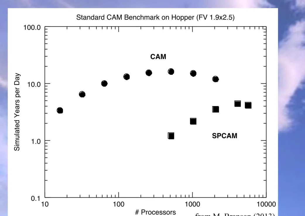
Finally, the SP-CAM is almost embarrassingly parallel, so that it can make efficient use of a very large number of processors. The reason is that the many copies of the CRM (one per CAM grid column) run independently, with no communication among themselves. As a result, for a given GCM grid spacing the SP-CAM can use many more processors than a conventionally parameterized model. Although the SP-CAM does much more arithmetic per simulated day than a conventionally parameterized GCM with the same resolution, the ability of the MMF to utilize more processors than a conventional GCM means that the wall-clock time required to complete a given simulation with the super-parameterization is only moderately longer than that required

with a conventional parameterization. An example is shown in Fig. 11. The MMF is orders of magnitude less expensive than a global cloud-resolving model (GCRM; e.g., Tomita et al., 2005).

Process models and global models

Over the past two decades, cloud-parameterization testing has become organized on an

international scale, beginning with NASA’s6 _FIRE7 _{program in the 1980s (Cox et al., 1987), and}

continuing in the 1990s and beyond with DOE’s8 _{ARM Program}9 _{(Stokes and Schwartz, 1994)}

Fig. 11: Plots of simulated years per wall-clock day versus the number of processors used, for the conventional CAM (black dots) and the SP-CAM (blue dots). The GCM grid spacing is 2.5º of longitude by 2º of latitude for both models. Note that the axes are logarithmically scaled. The figure shows that, with this resolution, the SP-CAM can efficiently use thousands of processors, while the CAM is limited to hundreds. The timing tests were performed on Hopper, a Cray XE6 at the National Energy Research Scientific Computer Center (NERSC), by Mark Branson of Colorado State University.

Standard CAM Benchmark on Hopper (FV 1.9x2.5)

10 100 1000 10000 # Processors 0.1 1.0 10.0 100.0

Simulated Years per Day

CAM

SPCAM

! Revised Tuesday, April 9, 2013! 19

6 _{NASA is the National Aeronautics and Space Administration.}

7 _{FIRE was the First ISCCP Regional Experiment; ISCCP is the International Satellite Cloud Climatology Project.}

8 _{DOE is the U.S. Department of Energy.}

9 _{Atmospheric Radiation Measurement Program.}

Super-Parameterization - Summary

• Runs like conventional parameterization: profile in, profile out; hence, the name, super-parameterization (term coined by David Randall);

• The CRMs do not communicate directly with each other (‘embarrassingly’ parallel problem);

• Radiation is usually computed on CRM grid; no cloud-overlap assumptions are needed;

• Momentum tendencies are not generally returned to GCM due to wrong momentum transport by 2D CRM; however use of 3D CRM is possible;

• Surface fluxes are still computed on GCM grid;

• Tendencies due to terrain are also due to GCM (no topography in CRM);

• PBL parameterization is generally off for scalars, but not wind;

• The width of the CRM domain is not tied to the GCM grid size (same way as a convective parameterization using no Δx information);

• GCM grid-cell should be large enough to contain large-scale convective systems.

CAM SP-CAM

Observations (Dai, 2001)

JJA Local Time of Precipitation Frequency Maximum

Text SP-CAM

Common bias (early maximum around noon) of many climate models

CAM

SP-CAM T85 (1.4x1.4o₎

Observations (Dai, 2001)

We still don’t understand why 4-km 2D CRM can do such a good job…

Diurnal cycle of precipitation

Eastward propagation of MCSs over US

SP-CAM5 SP-CAM3.5

SP-CAM3

CAM3 CAM5

Eastward propagation is robust in SP-CAM even at T42!

T42

T42 2x2.5o 2x2.5o 2x2.5o

Only large-scale processes are responsible for propagation of MCSs.

Precipitation over US

Li, Rosa, Collins & Wehner, 2012

SP-CAM is better than CAM to simulate the extreme precipitation

SP-CAM 2x2.5o CAM 2x2.5o

OBS

PDF of Rainfall

SP-CAM vs CAM T85

Zhou and Khairoutdinov 2015

Change of today’s extreme (99th) precipitation event frequency in RCP8.5 climate

Zhou and Khairoutdinov 2015

SP-CAM predicts much bigger increase in extreme precipitation frequency than CAM

SP-CAM 2x2.5o

CAM 2x2.5o

SP-CAM T85

MJO in SP-CAM T21

CAM SP-CAM

Randall, Khairoutdinov, Arakawa, Grabowski 2003

From the inception, SP-CAM/SP-CCSM has been arguably the best framework for MJO simulation

Pritchard 2012

SP-CAM NOAA OLR CAM

Khairoutdinov, DeMott, Randall 2008

W 2/m 4 W 2/m 4

MJO-event OLR anomalies 1986-2003

MMF

NOAA

JAN FEB MAR APR MAY JUN JUL AUG SEP OCT NOV DEC

JAN FEB MAR APR MAY JUN JUL AUG SEP OCT NOV DEC

El Nino La Nina Normal W 2/m 4 W 2/m 4

MJO-event OLR anomalies 1986-2003

MMF

NOAA

JAN FEB MAR APR MAY JUN JUL AUG SEP OCT NOV DEC

JAN FEB MAR APR MAY JUN JUL AUG SEP OCT NOV DEC

El Nino La Nina Normal

Seasonal Cycle of MJO _SP-CAM

NOAA

Zonal cross-section of MJO

Arnold et al, PNAS 2014

Arnold and Randall (2015)

Self-aggregation of convection on sphere SST=const, Solar=const, f=0

Thayer-Calder and Randall (2009)

Tropospheric moisture in Tropics binned by rainfall rate

In Obs and SP-CAM, heavy rainfall corresponds to regions with high humidity, especially in low-to-mid troposphere.

African Easterly Waves

McCary, Randall, Stan 2014

SP-CAM predicts much stronger increase in extreme precipitation frequency than CAM SP-CCSM @ T42

African Easterly Waves

McCary, Randall, Stan 2014

SP-CCSM couples convection and waves right to simulate AEWs even at T42! Again, as in MJO, mid-tropospheric moisture anomaly appears to be the key to

simulating AEWs.

OLR anomalies and 850 mb streamfunction and winds

ENSO

Super-parameterized GCMs

• 2001: SP-CAM

• 2007: SP-fvGCM: NASA GSFC (Wei-Kuo Tao)

• 2010: SP-WRF: (Stefan Tulich)

• 2011: SP-CFS: Indian Institute of Tropical Meteorology

CFS SP-CFS OLR, W/m2 OLR, W/m2 Prec mm/d CFS SP-CFS NOAA Goswami et al, JC (2015) SP-CFS (IITM)

SP-IFS - Super-parameterized IFS

• First implemented in OpenIFS, which is a free running IFS (cycle 38R1), but without data assimilation system;

• Summer 2014: T159 (~1.125o _{x 1.125}o_{) 3-year runs with}

SP-OIFS;

• Fall 2014: SP is implemented in IFS CY40R3.

• Fall 2014: SP is in IFS Single-Column Model CY40R1;

• Currently, implemented in CY41R3 and can be run using prepIFS system.

Anton Beljaars Glenn CarverFilip Vana Peter Bechtold

Preliminary results

using T159 SP-OpenIFS

• SP: 32 x 74; Δx=4 km; Δt=20s;

• All IFS cloud and convective parameterizations are off;

• PBL/mixing parameterizations are allowed;

• Radiation coupling through SP’s mean profiles (not on CRM grid as done in SP-CAM);

SP-OIFS

OIFS GPCP (OBS)

JJA Precipitation T159

Mean climatology of SP-IFS doesn’t look bad for a model which hasn't been properly tuned.

Frequency Spectrum (Subseasonal): Precipitation in Tropics (15o_S-15o_N) IFS SP-IFS GPCP IFS SP-IFS GPCP Symmetric Anti-Symmetric

Anti-Symmetric Symmetric IFS SP-IFS GPCP IFS SP-IFS GPCP Frequency Spectrum (S/N): Precipitation in Tropics (15o_S-15o_N)

TRMM  

IFS  

SP-­‐IFS  

Summer  (May-­‐Oct)       Winter  (Nov-­‐Apr)   Variance:  20-­‐100  day  filtered  precipitation

Summer&(May+Oct)& & &Winter&(Nov+Apr)&& Variance:&20+100&day&filtered&U850& &ERA40& & & & & &&IFS& & & & & & &&SP+IFS& & & & & &

Lag$correla*on$(U850,$Winter)$ MJO$eastward$propaga*on$ $IFS $ $ $ $ $$$SPAIFS$ ERA40! Reference$domain:$ 1.25SA16.25N,$68EA96E! *!US!CLIVAR!MJO!Diagnos5c!metrics!

Lag$correla*on$(U850,$Summer)$ Summer$ISO$northward$propaga*on$ $IFS $ $ $ $ $$$SP?IFS$ ERA40! Reference$domain:$ 3.75N?21.25N,$68E?96E!

IFS

Tuning for cloud fraction using SCM IFS (TWP ICE case)

SP-IFS (before tuning)

Bias in OLR in SP-IFS CY40R1 forecast

SP-IFS (after tuning)

Bias in OLR in SP-IFS CY40R1 forecast

IFS

Shortwave bias

SP-IFS with reduced IceFall rate and CWP threshold SP-IFS (Marat’s run, Default setting ? )

What have we learnt from SP?

Even small-domain 2D CRM works better than current

convective parameterizations to represent variability of climate system on various timescales.

We know much more about MJO now thanks to the SP.

As the SP interacts with a GCM as an ordinary parameterization (1D profile in, 1D profile out), it is in principle possible to develop a parameterization that works as well as the SP.

http://www.cmmap.org/research/pubs-mmf.html Lots of MMF publications: