Estimating Output Gap, Core Inflation, and the NAIRU for Peru

(1)

BANCO CENTRAL DE RESERVA DEL PERÚ

Estimating Output Gap, Core Inflation, and the

NAIRU for Peru

Gabriel Rodríguez

*

* Central Reserve Bank of Peru and Pontificia Universidad Católica del Perú

DT. N° 2009-011

Serie de Documentos de Trabajo

Working Paper series

Abril 2009

Los puntos de vista expresados en este documento de trabajo corresponden a los autores y no reflejan necesariamente la posición del Banco Central de Reserva del Perú.

The views expressed in this paper are those of the authors and do not reflect necessarily the position of the Central Reserve Bank of Peru.

(2)

Estimating Output Gap, Core In‡ation, and the

NAIRU for Peru

Gabriel Rodríguezy

Department of Research, Central Bank of Peru Ponti…cia Universidad Católica del Perú

This Version: April 17, 2009

Abstract

Following Doménech and Gómez (2006), and using quarterly Peruvian data for 1970:1-2007:4, I estimate a model that exploits the informa-tion contained in the in‡ainforma-tion, unemployment and private investment rates in order to estimate non-observable variables as output gap, the NAIRU and the core in‡ation. The unknown parameters are esti-mated by maximun likelihood using a Kalman …lter initialized with a partially di¤use prior, and the unobserved components are estimated using a smoothing algorithm. The results suggest that only the in‡a-tion rate contains useful informain‡a-tion in order to estimate the output gap. Estimates suggest poor performance for the unemployment and private investment rates. I explain this issue as related to the poor quality of the construction of these variables. In order to perform a sensitivity analysis, I estimate the output gap using other alternative methods. The correlations are very di¤erent and very far away from the estimates obtained in this paper. It is clear that estimates obtained from simple statistical …lters give poor approximations.

Keywords: Potential Output, Core In‡ation, NAIRU, Latent Vari-ables, Investment.

JEL Classi…cation: C22, C32, C52, E31, E32.

I thank useful comments from participants to the XXV Meeting of Economists of the Central Bank of Peru in December 2007. I also thanks Marco Vega for useful comments. The views expressed in this paper are those of the author and do not re‡ect necessarily the position of the Central Bank of Peru.

y_{Address for Correspondence:} _{Gabriel Rodríguez, Banco Central de Reserva del}

Peru, Subgerencia de Investigación Económica, 441-445 Jr. Miroquesada, Lima 1, Lima-Peru. Telephone: +511-613-2000 (3970), Fax: +511-613-2516, E-Mail address: [email protected].

(3)

1 Introduction

There are many reasons to decompose output into its trend and cyclical com-ponents. However, in order to be a useful decomposition, it should account for three central stylized facts in modern macroeconomics. The …rst one is the negative correlation between the output gap and the deviation of the unemployment rate from the structural rate of unemployment (or NAIRU). This relationship is usually referred to as Okun’s Law. The second stylized fact is the trade-o¤ in the short run between in‡ation and unemployment. The third stylized fact is the comovement of output and investment. Some authors as Stadler (1994), Burnside (1998) and Canova (1998) consider that this relationship is one of the most important regularities independently of the detrending method. Considering investment is more volatile than out-put, the investment rate increases in expansions and falls in recessions.

The stylized facts above mentioned indicate that there is important in-formation in the unemployment, in‡ation and investment rates in order to measure the cyclical position of the economy, and therefore, of the output gap. In a recent paper, Doménech and Gómez (2006) take into consideration these factors and propose and estimate an unobserved component model for the US which allow to obtain time-varying estimates of the NAIRU, core in‡ation and the structural investment rate which are compatible with the usual decomposition of the GDP into trend and cycle.

I consider that the approach of Doménech and Gómez (2006) exploits more useful information compared with other approaches in the literature. In other words, other approaches have omitted at least one of the three stylized facts above mentioned. For example, Kuttner (1994) uses only in-formation contained in in‡ation through a simple backward-looking version of the Phillips curve. Apel and Jansson (1999), Camba-Méndez and Palen-zuela (2003) and Fabiani and Mestre (2004) do not consider the investment rate and their estimated Phillips curve does not include anytime-varying

(4)

component which proxies core or expected in‡ation. On the other side, Ger-lach and Smets (1999) consider only a backward-looking Phillips curve and an aggregate demand equation which relates the output gap to its own lags and real interest rate. Laubach (2001) has proposed a model using only a Phillips curve linking the …rst di¤erence of in‡ation to cyclical unemploy-ment and the equations needed to model the two unobservable components (the NAIRU and the gap) of the unemployment rate. The model is very close to the one proposed by Gordon (1997), but allowing the NAIRU to be a non-stationary process in some countries. In a very similar framework, Staigner, Stock and Watson (2001) uses the information contained in the in-‡ation rate and the growth of real wages to calculate a time-varying estimate of the NAIRU.

Following Doménech and Gómez (2006), I estimate a model that exploits the information contained in the in‡ation, unemployment and private invest-ment rates in order to estimate some non observable variables as output gap, the NAIRU and core in‡ation. In fact this is a model of four equations. One is the model for the potential output. The second equation is the Okun’s Law. The third and fourth equations are for the unemployment and private investment rates. The period of estimation is 1970:1-2007:4.

The results suggest that only the in‡ation rate contains useful informa-tion to estimate the output gap. Estimates suggest poor performance for the unemployment and private investment rates. It is unfortunate because the approach of Doménech and Gómez (2006) suggest the importance of these two variables to obtain a more reliable estimate of the output gap. I explain this issue as related to the poor quality in the construction of these variables. The standard picture of these variables suggests the presence of anomalies. However, at theoretical level, this fact does not invalidate the potential utility of these two variables in estimating the output gap as suggested by Doménech and Gómez (2006).

(5)

using some statistic …lters. I use Hodrick and Prescott (1997), Baxter and King (1999), Christiano and Fitzgerald (2003), Beveridge and Nelson (1981). Furthermore I estimated the output gap using the approach of Clark (1987). I also estimate the output gap using a simple linear trend, and a quadratic trend. Finally, I compare the output gap obtained in this paper with the output gap obtained in Rodríguez (2009) and with the output gap obtained using a model with two variables, that is, excluding unemployment and private investment rates. The …rst comment from these correlations is the fact that all them are very di¤erent and very far away from the estimates obtained in this paper. It is clear that estimates obtained from simple statistic …lters gives a poor approximation. Another comment is that some simple estimators like a linear trend or a quadratic trend perform better that simple statistical …lters. The highest correlation is obtained when the output gap is calculated using the approach of Clark (1987) which is an approach more acceptable from the economic perspective.

The document has the following sections. In Section 2, the model is presented. Section 3 discusses some estimation issues. Section 4 presents and discusses the results. Section 5 concludes.

2 The Model

2.1 The Potential Output

In order to model the log of real GDP, yt, I start with the descomposition due to Watson (1986):

yt=yt+yct; (1) where y_t is the trend component and yc

t is the cyclical component. This approach is also used by Kuttner (1994) and many others. The cycle is assumed to follow a stationary AR(2) model with complex roots:

(6)

where_f!ytg i:i:d: N(0; 2!y); 22[ =20; =3];and 0< 1 <1:

Unit root statistics suggest the presence of a unit root in output. Ac-cording to Harvey (1987), a su¢ cient condition for model (1) to be identi…ed is that the order of the moving average component of y_t is less that of its autoregressive part, including the unit roots. This consideration then lead to the following speci…cation:

y_t= _y+! t; (3)

where _y is a drift term, and _f! tg i:i:d: N(0; 2! ) which is uncorrelated with_f!ytg:

Even when the residuals seem to have no autocorrelation, they do show some heteroscedasticity. At this respect Stock and Watson (2002) found no change in the autoregressive parameters of the output gap but did …nd a break in the output gap volatility. I may incorporate volatility breaks for the Peruvian economy. I accomplish this by allowing the parameter !y to vary with time. That is, I use !yt = !y1 ift <1990 : 3 and !yt = !y2 ift 1990 : 3.

2.2 The Phillips Curve

A simple speci…cation of the new Phillips curve is due to Galí and Gertler (1999). This curve assumes proportionality between marginal cost and the output gap:

t= ytc+ Et( t+1); (4) where t is the in‡ation rate, yct is the output gap, Et(:) is the expectation operator based on information up to and includingt, and are constants. Following the considerations established in Theorem 2 of Doménech and Gómez (2006), the equation for in‡ation is given by

t= (1

X

i11

(7)

where t is the rate of in‡ation rate,ytc is the output gap, y is a constant, fv tg i:i:d: N(0; 2v ); (L) =

P

i11 iLi; is the long-run in‡ation rate, t = ! t; f! tg i:i:d: N(0, 2! ); and fv tg;f! tg; and fytcg are mutually uncorrelated.

As with output, the residuals show some heteroscedasticity. This in agreement with Sensier and Van Dijk (2004) who …nd several breaks in in‡ation volatility. I …nd two breaks in in‡ation volatility, in 1988:3 and 1990:3, that I have incorporated in the model. I have accomplished this by allowing the parameter ! to vary with time. That is, instead of ! , I use ! t = ! 1 ift <1988 : 3, ! t= ! 2 if1988 : 3 t <1990 : 3;and

! t= ! 3 ift 1990 : 3.

2.3 The Okun’s Law

Some empirical evidence suggests a relationship between output and unem-ployment. This relationship, known as Okun’s Law has been used by several authors to asses the cyclical position of the economy; see for example Clark (1989), Blanchard and Quah(1989). I do account for the negative correla-tion between the output gap and cyclical unemployment by means of the following equation:

Ut= uUt 1+ (1 u)Ut+ y(L)ytc+vut; (6)

whereUt is the trend component, fvutg i:i:d: N(0; 2uv); y(L) is a poly-nomial in the lag operator such that _y(1)<0:

Unlike Apel and Jansson (1999) and Camba-Méndez and Palenzuela (2003), I allow the output gap to a¤ect the unemployment with some lags as the empirical evidence seems to suggest. The NAIRU, Ut;is allowed to be a process I(1) or I(2). That is,

Ut = ut+Ut 1; (7)

(8)

where06 _u 61;_f!utg is i:i:d: N(0, 2!u): If u = 1therefore Ut is I(1); if _u= 0 therefore Ut is I(1). Estimations suggest the last alternative:

2.4 The Investment

One of the most important regularities found by the empirical research on business cycles is that investment strongly co-moves with output but with more volatility; see Canova (1998), Burnside (1998), Harvey an Trimbur (2003). This stylized fact implies that the deviations of the investment rate, from its long-run trend, is markedly procyclical. Therefore, I model the co-movement of the investment rate with the output gap by the following equation:

xt= xxt 1+ (1 x)xt+ y(L)ytc+vxt; (9) where_fvxtg i:i:d: N(0; 2xv); y(L) is a polynomial such that y(1)>0:

As for the unemployment rate, the trend component of the investment rate is allowed to be an I(1) or I(2) processes. That is,

xt = xt+xt 1 (10)

xt = x xt 1+!xt (11)

where06 _x61;_f!xtg i:i:d: N(0; 2!x):If x= 2!x = 0;thenxtis equal to a constant. Estimations suggest the previous alternative:

3 Estimation Issues

I follow the approach of Doménech and Gómez (2006). That is, to cast the model into state-space form and use the Kalman …lter for likelihood evaluation. The algorithm includes the use of a smoothing algorithm to obtain estimates of the unobserved components together with their mean squared errors.

According to preliminar analysis, all variables are modeled as I(1), with only the output having a drift term. The parameters !y and ! are time-varying according to the breaks. In addition, we specify a degree zero the

(9)

polynomial _y(L), degree 1 for the polynomial _y(L), and degree 4 for the polynomial (L), and we include three outliers identi…ed for in‡ation in the model.

The model may be put into state-space form. De…ne the following ma-trices: W = 2 6 6 6 6 6 6 6 6 4 1 0 0 0 0 0 0 0 0 0 0 0 0 0 0 0 0 0 0 0 0 0 0 0 0 0 0 0 3 7 7 7 7 7 7 7 7 5 ,T = 2 6 6 6 6 6 6 6 6 4 1 0 0 0 0 0 0 0 1 0 0 0 0 0 0 0 1 0 0 0 0 0 0 0 1 0 0 0 0 0 0 0 0 1 0 0 0 0 0 0 0 1 0 0 0 0 0 2₁ 2 1cos 2 3 7 7 7 7 7 7 7 7 5 , t= 2 6 6 6 6 6 6 6 6 4 y_t Ut xt t yc_t ₂ yc_t ₁ yc t 2 3 7 7 7 7 7 7 7 7 5 ; Ht= 2 6 6 6 6 6 6 6 6 4 !y 0 0 0 0 0 0 0 0 _!u 0 0 0 0 0 0 0 0 _!x 0 0 0 0 0 0 0 0 _{! t} 0 0 0 0 0 0 0 0 0 0 0 0 0 0 0 0 0 0 0 0 0 0 0 0 0 0 0 _!yt 3 7 7 7 7 7 7 7 7 5 ; Z= 2 6 6 4 1 0 0 0 0 0 1 0 1 _u 0 0 0 0 ₀ 0 0 1 _x 0 0 _y₁ _y₀ 0 0 0 1 P4₌₁ _i 0 0 _y 3 7 7 5; Xt= 2 6 6 4 0 0 0 0 0 0 0 0 0 0 0 0 0 o1t o2t o3t 3 7 7 5; G= 2 6 6 4 0 0 0 0 0 0 0 0 0 0 0 0 _uv 0 0 0 0 0 0 0 0 _xv 0 0 0 0 0 0 0 0 1 0 3 7 7 5; where _!y = !y= v, !u = !u= v, !x = !x= v; ! t = ! t= v; !yt = !yt= v; uv = uv= v; xv = xv= v: The oit variables (i =

1;2;3) model the three outliers that a¤ect in‡ation rate. Then t is the state vector, the parameter 2_v is concentrated out of the likelihood, and the state-space equations are

t+1 = W +T t+Ht t (12)

(10)

wherezt= [yt; Ut uUt 1; xt xxt 1; t P4_i₌₁ i t i]0, = ( y; o1; o2; o3)0 is the vector of regression coe¢ cients andV ar( t) = 2vI: The parameters in are also concentrated out of the likelihood. The …lter starts …ltering att= 5 because we condition on the …rst four non missing observations of each series.

The previous state-space model is non-stationary and the initial condi-tions for the Kalman Filter are not well de…ned. To …x this inconvenient, I use the approach of De Jong (1991). According to this approach, the initial state vector 1is modelled as partially di¤use and an augmented Kalman …l-ter algorithm called the “di¤use Kalman …l…l-ter”is used to handle the di¤use part. As shown by De Jong and Chu-Chun-Lin (1994), the di¤use Kalman …lter can be collapsed to the ordinary Kalman …lter after a few iterations. The di¤use Kalman …lter can be used to evaluate the likelihood and thus the model parameters can be estimated by maximum likelihood.

After having estimated the model parameters, I can use a smoothing algorithm to have two-sided estimates of the unobserved components and their mean squared errors. To do it, I use the algorithm proposed by De Jong and Chu-Chun-Lin (1993). The di¤use part is = [y₀; U0; x0; 0]0, so the initial state is 1 =A +W +[0; x01]0, whereA= [I;0]0andx1= [yc1; y0c; yc1]0 has a known (stationary) distribution. For further details consult Doménech and Gómez (2006).

4 Results

Estimations are based on quarterly Peruvian data for the period 1970:1-2007:4. The data includes real GDP, in‡ation, unemployment and private investment rates. Table 1 presents the estimates of the di¤erent model parameters, together with their t-statistics in parenthesis. It is seen that our estimation of the output gap is close to the 5% of signi…cance in the Okun’s Law ( _y₀). It is very signi…cant in the Phillips curve. However, there appears no signi…cant in the investment equation. This suggests that

(11)

the in‡ation rate contain very useful information about the cyclical position of the economy. However it appears not to be signi…cant information in the unemployment and investment rates.

The results in the …rst two columns of Table 1 show that there is indeed a break at 1990:3 in the output gap volatility, measured by the standard deviation !yt. The standard deviation has sharply declined from 0.031 before 1990:3 to 0.018 afterwards.

The results for the Okun’s Law indicate that there is close to 5% of signi…cance contemporaneous e¤ect of business cycles on the unemployment rate. Another noteworthy result is about the magnitude and the signi…cance of vu. It is not signi…cant so that the Okun’s Law almost …ts completely the unemployment rate. In the case of the investment rate the contemporaneous correlation with the output gap is not signi…cant but there is a intermediate inertia given by _x. Because the standard deviation of vx is small (1.2%), the decomposition between trend and cycle accounts almost entirely for the variation of the investment rate.

The last four columns of Table 1 present the estimation results for the Phillips curve. The model performs well in explaining the dynamics of in-‡ation in Peru. The output gap is signi…cant suggesting that most of the business cycles ‡uctuations have been associated with procyclical behavior of in‡ation. From the results in Table 1 we see the that forward looking behavior is more important that the backward looking behavior (0.794 and 0.206, respectively).

As with the GDP, I have found two breaks in in‡ation volatility, mea-sured by the standard deviation ! . They occurs in 1988:3 and 1990:3. From the results of Table 1, there is a huge increase in in‡ation volatility from 1988:3 to 1990:3. After it, we observe a dramatic reduction in in‡ation volatility.

An important conclusion from the above results is the reduced or null information in the unemployment and private investment rates useful to

(12)

es-timate the output gap or the potential output. It appears that only in‡ation contains useful information to estimate the output gap. The only explana-tion I have for this issue is the bad construcexplana-tion of the unemployment rate. Its construction or estimation is very bad and it may be observed in the Figure 1. Its oscillations are not due to seasonal behavior because the series shown in Figure 1 has been seasonal adjusted. This inability of the unem-ployment rate to help in estimation of the output gap is important because it preludes the potential estimation of a reliable NAIRU. With the current data we are unable to perform some estimations with some degree of relia-bility. A similar set of inconveniencies are found for the private investment rate. The quality of this variable is poor and consequently the information useful to estimate the output gap is very limited.

What is said above is unfortunate because the approach used in the paper tries to exploit useful information in unemployment and private investment rates in order to estimate the output gap. It appears that only in‡ation rate has useful information to estimate the output gap which is coherent with Kuttner (1994). These issues show the important di¢ culties that some countries like Peru may face in order to estimate important unobservable variables like NAIRU, private invest rate, core in‡ation and output gap. What is important to say is that the empirical evidence does not invalidate the approach of Doménech and Gómez (2006) concerning the importance of the unemployment and private investment rates. We insist in a problem with the quality of the information which does not invalidate the theoretical approach of Doménech and Gómez (2006).

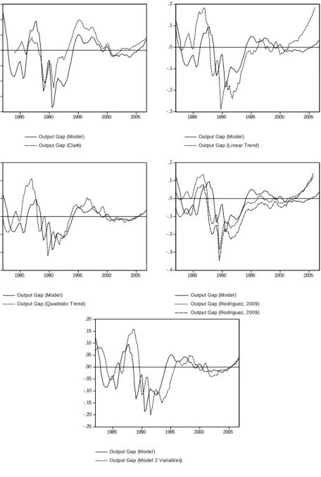
In order to perform a sensitivity analysis, I estimate the output gap using some statistic …lters. I use Hodrick and Prescott (1997), Baxter and King (1999), Christiano and Fitzgerald (2003), Beveridge and Nelson (1981). Furthermore I estimated the output gap using the approach of Clark (1987). I also estimate the output gap using a simple linear trend, and a quadratic trend. Finally, I compare the output gap obtained in this paper with output

(13)

gaps obtained in Rodríguez (2009) and with the output gap obtained using a model with two variables, that is, excluding unemployment and private investment rates. The correlations are HP (0.406), BK (0.416), CF (0.136), BN (-0.149), Clark (0.771), LT (0.558), QT (0.613), Rodríguez (0.464 and 0.512). The …rst comment from these correlations is the fact that all them are very di¤erent and very far away from the estimates obtained in this paper. It is clear that estimates obtained from simple statistic …lters gives a poor approximation. Another comment is that some simple estimators like a linear trend or a quadratic trend perform better that simple statistical …lter like HP, BK, BN or CF. The highest correlation is obtained when the output gap is calculated using the approach of Clark (1987) which is an approach more acceptable from the economic perspective.

5 Conclusions

Following Doménech and Gómez (2006), I estimate a model that exploits the information contained in the in‡ation, unemployment and private in-vestment rates in order to estimate some non observable variables as output gap, the NAIRU and the core in‡ation. In fact this is a model of four equa-tions. One is the model for the potential output. The second equation is the Okun’s Law. The third and fourth equations are for the unemployment and private investment rates.

The results suggest that only the in‡ation rate contains useful infor-mation in order to estimate the output gap. Estimates suggest poor perfor-mance for the unemployment and private investment rates. It is unfortunate because the approach of Doménech and Gómez (2006) suggest the impor-tance of these two variables to obtain a more reliable estimate of the output gap. I explain this issue as related to the poor quality of these variables in their construction. The standard picture of these variables suggests the presence of anomalies. This fact does not invalidate the potential utility of these two variables in estimating the output gap as suggested by Doménech

(14)

and Gómez (2006).

In order to perform a sensitivity analysis, I estimate the output gap using some statistic …lters. I use Hodrick and Prescott (1987), Baxter and King (1999), Christiano and Fitzgerald (2003), Beveridge and Nelson (1981). Fur-thermore, I estimated the output gap using the approach of Clark (1987). I also estimate the output gap using a simple linear trend, a quadratic trend. Finally, I compare the output gap obtained in this paper with output gap obtained in Rodríguez (2009) and with the output gap obtained using a model with two variables, that is, excluding unemployment and private in-vestment rates. The …rst comment from these correlations is the fact that all them are very di¤erent and very far away from the estimates obtained in this paper. It is clear that estimates obtained from simple statistic …lters gives a poor approximation. Another comment is that some simple esti-mators like a linear trend or a quadratic trend perform better that simple statistical …lter like HP, BK, BN or CF. The highest correlation is obtained when the output gap is calculated using the approach of Clark (1987) which is an approach more acceptable from the economic perspective.

References

[1] Apel, M., and Jansson, P. (1999), “A Theory-Consistent System Ap-proach for Estimating Potential Output and the NAIRU”, Economic Letters 64, 271-275.

[2] Baxter, M. and R. G. King (1999), “Measuring Business Cycles: Ap-proximate Band-Pass Filter for Economic Time Series,”The Review of Economics and Statistics 79, 551-563.

[3] Beveridge, S., and C. Nelson (1981), “A New Approach to the Decom-position of Economic Time Series into Permanent and Transitory

(15)

Com-ponents with Particular Attention to the Measurement of the Business Cycle,”Journal of Monetary Economics 7, 151-174.

[4] Blanchard, O. J., and Quah, D. (1989), “The Dynamic E¤ects of Aggre-gate Demand and Supply Disturbances,”American Economic Review

79, 655-673.

[5] Burnside, C. (1998), “Detrending and Business Cycles Facts: A Com-ment”,Journal of Monetary Economics 41, 513-532.

[6] Burns, A. F., and W. C. Mitchell (1946), Measuring Business Cycles, New York, NBER.

[7] Camba-Méndez, G., and Palenzuela, D. R. (2003), “Assessment Criteria for Output Gap Estimates”, Economic Modelling 20, 529-562.

[8] Canova, F. (1998), “Detrending and Business Cycle Facts”,Journal of Monetary Economics 41, 475-512.

[9] Clark, P. (1987), “The Cyclical Component of US Economic Activity,”

Quarterly Journal of Economics 102, 797-814.

[10] Clark, P. (1989), “Trend Reversion in Real Output and Unemploy-ment„”Journal of Econometrics 40, 14-32.

[11] Christiano, L. J., and T. J. Fitzgerald (2003). “The Band Pass Filter,”

International Economic Review 44(2), 435-465.

[12] De Jong, P. (1991), “The Di¤use Kalman Filter”, Annals of Statistics

19, 1073-1083.

[13] De Jong, P., Chu-Chun-Lin, S. (1994), “Fast Likelihood Evaluation and Prediction for Nonstationary State Space Models,”Biometrika 81, 133.142.

(16)

[14] De Jong, P., and Chu-Chun-Lin (2003), “Smoothing with an Unknown Initial Condition”, Journal of Time Series Analysis 24, 141-148.

[15] Doménech, R. and Gómez, V. (2006), “Estimating Potential Output, Core In‡ation, and the NAIRU as Latent Variables,”Journal of Busi-ness and Economic Statistics 24(3), 354-365.

[16] Fabiani, S., and Mestre R. (2004), “A System Approach for Measuring the Euro Area NAIRU,”Empirical Economics 29, 311-341.

[17] Galí, J., and Smets, F. (1999), “In‡ation Dynamics: A Structural Econometric Analysis,”Journal of Monetary Economics 44, 195-222.

[18] Gerlach, S., and Smets, F. (1999), “Output Gaps and Monetary Policy in the EMU Area,”European Economic Review 43,801-812.

[19] Gordon, R. J. (1997), “The Time-Varying NAIRU and Its Implications for Economic Policy,”Journal of Economic Perspectives 11, 11-32.

[20] Harvey, A. C. (1987), Forecasting Structural Models and the Kalman Filter, UK: Cambridge University Press.

[21] Harvey, A. C. and Trimbur, T. M. (2003), “General Model-Based Fil-ters for Extracting Cycles and Trands in Economic Time Series,”The Review of Economics and Statistics 85, 244-255.

[22] Hodrick, R. and E. Prescott (1997), “Postwar US Business Cycles: An Empirical Investigation,”Journal of Money, Credit and Banking 29 ,1-16.

[23] Keynes, J. M. (1936), The General Theory of Employment, Interest, and Money. London: MacMillan.

[24] Kuttner, K. N. (1994), “Estimating Potential Output as a Latent Vari-able”, Journal of Business and Economic Statistics 12, 361-368.

(17)

[25] Laubach, T. (2001), “Measuring the NAIRU: Evidence from Seven Economies”, Review of Economics Studies 83, 218-231.

[26] Rodríguez, G. (2009), “Using a Forward-Looking Phillips Curve to Es-timate the Output Gap in Peru,” Unpublished manuscript.

[27] Sensier, M., and D. van Dijk (2004), “Testing for Changes in Volatil-ity of US Macroeconomic Time Series”, The Review of Economic and Statistics.86, 833-839.

[28] Stadler, G. W. (1994), “Real Business Cycles,”Journal of Economic Lietrature 38, 1750-1783.

[29] Staigner, D., Stock, J. H., and Watson, M. W. (2001), “Prices, Wages and the US NAIRU in the 1990s,” Working Paper 8320NBER. [30] Stock, J. H., and Watson, M. W. (1998), “Median Unbiased Estimation

of Coe¢ cient Variance in a Time-Varying Parameter Model”, Journal of the American Statistical Association 93, 349-358.

[31] Stock, J. H., and Watson, M. W. (2002), “Has the Business Cycle Changed and Why”, NBER Macroeconomics Annual, 159-218.

[32] Watson, M. W. (1986), “Univariate Detrending Methods with Stochas-tic Trends,”Journal of Monetary Economics 18, 29-75.

(18)

Table 1. Maximum Likelihood Parameter Estimates Equation

Output Okun’s Law Investment Phillips Curve 1 0.697 y0 -0.066 y0 0.040 y -0.902 o1 3.405 (11.44) (-1.88) (0.78) (-2.39) (12.60) 2 0.233 u 0.246 y1 0.091 1 0.067 o2 1.670 (2.15) (1.12) (1.48) (9.81) (1.90) y 0.006 vu 0.002 x 0.628 2 0.073 o3 7.777 (3.46) (1.06) (10.55) (11.45) (160.66) !y1 0.031 !u 0.009 vx 0.012 3 0.024 ! 1 0.342 (5.13) (5.00) (8.63) (3.95) (5.57) !y2 0.013 !x 0.003 4 0.041 ! 2 1.563 (4.18) (1.79) (6.67) (3.63) ! 0.018 v 0.037 ! 3 0.021 (5.07) (2.64)

(19)

9.8 10.0 10.2 10.4 10.6 10.8 1980 1985 1990 1995 2000 2005 Log of Real GDP -2 0 2 4 6 8 10 1980 1985 1990 1995 2000 2005 Inflation Rate .04 .06 .08 .10 .12 1980 1985 1990 1995 2000 2005 Unemployment Rate .100 .125 .150 .175 .200 .225 .250 1980 1985 1990 1995 2000 2005 Private Investment Rate

(20)

9.8 9.9 10.0 10.1 10.2 10.3 10.4 10.5 10.6 10.7 1985 1990 1995 2000 2005 L o g o f Re a l G DP Po t e n t i a l G DP -2 0 2 4 6 8 10 1985 1990 1995 2000 2005 In f la t io n Ra t e Co r e In f la t io n .04 .05 .06 .07 .08 .09 .10 .11 .12 1985 1990 1995 2000 2005 Unemployment Rate Trend Component .10 .12 .14 .16 .18 .20 .22 .24 .26 1985 1990 1995 2000 2005 Private Investment rate

Trend Component

Figure 2. Current and Trend Components (Output, In‡ation, Unemployment, Private Investment)

(21)

-.20 -.15 -.10 -.05 .00 .05 .10 .15 .20 1985 1990 1995 2000 2005 Output Gap (Model)

Output Gap (Hodrick-Prescott)

-.20 -.15 -.10 -.05 .00 .05 .10 .15 1985 1990 1995 2000 2005 Output Gap (Model)

Output Gap (Baxter-King)

-.20 -.15 -.10 -.05 .00 .05 .10 .15 1985 1990 1995 2000 2005 Output Gap (Model)

Output Gap (Christiano-Fitzgerald)

-.20 -.15 -.10 -.05 .00 .05 .10 .15 1985 1990 1995 2000 2005 Output Gap (Model)

Output Gap (Beveridge-Belson)

(22)