Heating Augmentation for Short Hypersonic
Protuberances
Ali R. Mazaheri
∗and William A. Wood
†Computational aeroheating analyses of the Space Shuttle Orbiter plug repair models are validated against data collected in the Calspan University of Buffalo Research Center (CUBRC)48inchshock tunnel. The comparison shows that the average difference between computed heat transfer results and the data is about 9.5%. Using CFD and Wind Tunnel (WT) data, an empirical correlation for estimating heating augmentation on short hyper-sonic protuberances (k/δ < 0.3) is proposed. This proposed correlation is compared with several computed flight simulation cases and good agreement is achieved. Accordingly, this correlation is proposed for further investigation on other short hypersonic protuberances for estimating heating augmentation.
Nomenclature
Symbols
Cp Specific heat, [BT U/slugsR]
d Plug repair diameter, [inches] k Protuberance height, [inches]
M Mach number
p Pressure, [lb/f t2]
q Heat transfer rate, [BT U/f t2·sec]
r Constant
Re Unit Reynolds number, [1/f t]
St Stanton number
T Temperature, [R] V Total velocity, [f t/sec] x, y, z Coordinate system, [inches] α Angle-of-attack, [degrees] δ BL thickness, [inches]
δ∗ Displacement thickness, [inches]
Emissivity
µ Viscosity, [lb·sec/f t2] ρ Density, [slugs/f t3]
θ Momentum thickness, [inches] Subscripts
∞ Free-stream
i, j, k Grid points indices
p Plug repair
rf Recover factor
t Total
θ Momentum thickness
w Wall
x, y, z Local x-, y-, z-coordinate < . > Average value
Acronyms
BF Bump factor
BL Boundary layer
WLE Wing leading edge
WT Wind tunnel
Introduction
Following the Shuttle Columbia accident in 2003, NASA investigated methods for performing on-orbit repairs to the Thermal Protection System (TPS) and their impacts on the aerothermodynamic environment of the Space Shuttle Orbiter experienced during re-entry.1 Various methods were developed to repair damaged areas of the Space Shuttle Orbiter, including the use of tile repairs and plug repairs that are used on-orbit to patch small breaches on the Orbiter tile and on the Wing Leading Edge (WLE) Reinforced Carbon-Carbon (RCC) panels, respectively. Several studies have been reported for the aeroheating analysis of the tile and
∗AMA, Inc./NASA LaRC, Aerothermodynamics Branch, AIAA Member;[email protected]
†NASA Langley Research Center, Aerothermodynamics Branch, Lifetime AIAA Member;[email protected]
Copyright c2008 by the American Institute of Aeronautics and Astronautics, Inc. The U.S. Government has a royalty-free license to exercise all rights under the copyright claimed herein for Governmental purposes. All other rights are reserved by the copyright owner.
plug repairs (see Ref.2–7) However, no correlation has been reported to estimate the augmented maximum heating resulting from disturbing the local flow field.
The aim of this investigation is to obtain a heating augmentation correlation for a hypersonic repair surface using flow field information around the smooth Outer Mold Line (OML) of the vehicle. The focus of this study is on the Space Shuttle Orbiter. Aerothermodynamic computations are studied for wind tunnel swept cylinder models with rounded protuberance of different heights is placed on the cylinder. CFD simulations are obtained for the WT cases and the results are compared with the WT data. Based on CFD and WT data, a simple heating augmentation correlation is proposed for comparison with several flight CFD data. The correlation does require that Shuttle Smooth OML results are available.
CFD Validation
In this section, computational analysis are validated against available wind tunnel data. The valida-tion is necessary in order to extrapolate the CFD data to flight condivalida-tions for which a heating correlavalida-tion augmentation is needed.
Computational Procedures
Figure 1. Schematic of the wind tunnel model. Computational aerothermodynamic analyses are
conducted using Langley Aerothermodynamic Up-wind Relaxation Algorithm (LAURA),8, 9 which is a chemically reacting viscous flow solver. Compu-tations are performed for three-dimensional swept cylinder models, which are shown schematically in Figures1 and2.
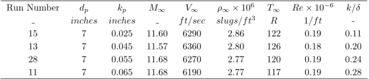
Several different plug heights are considered. The plug dimensions and wind tunnel flow condi-tions corresponding to the experimental run num-bers are given in Table 1. Perfect gas air is used during the experiments. Experiments are conducted by Calspan University of Buffalo Research Center (CUBRC)10 in a 48 inch shock tunnel. Computa-tions are simulated at the wind tunnel condiComputa-tions with a perfect gas air model.
Table 1. Plug dimensions and wind tunnel flow conditions corresponding to the experimental run numbers.
Run Number dp kp M∞ V∞ ρ∞×106 T∞ Re×10−6 k/δ
inches inches f t/sec slugs/f t3 R 1/f t
-15 7 0.025 11.60 6290 2.86 122 0.19 0.11
13 7 0.045 11.57 6360 2.80 126 0.18 0.20
28 7 0.055 11.68 6270 2.77 120 0.19 0.24
11 7 0.065 11.68 6190 2.77 117 0.19 0.28
Because each WT model was individually manufactured, a specific grid was needed for each of the models to account for their precise features. A grid topology was designed to generate smooth grids that can capture geometrical features of the model and physical behavior of hypersonic flow around the body. A schematic of the developed viscous grid is shown in Figure3. More details of the grid generating techniques are reported in Ref.12
Computational Results
Wind tunnel models, each consisting of a 7 inch rounded plug on a swept cylinder with a blunted nose, shown in Figures 1 and 2, are analyzed at the wind tunnel conditions given in Table1. As stated before, perfect gas air is used for both wind tunnel experiments and computations. Simulations are conducted with
Cavity Plug
Flow direction
Not to scale. Exaggerated to show contour.
Figure 2. Schematic of the plug shape with its cavity.
X Y Z X Y Z X Y Z X Y Z
the WT conditions for which the surface temperatures are relatively constant (cold wall). WT conditions are considered laminar and therefore only laminar flow is computed.
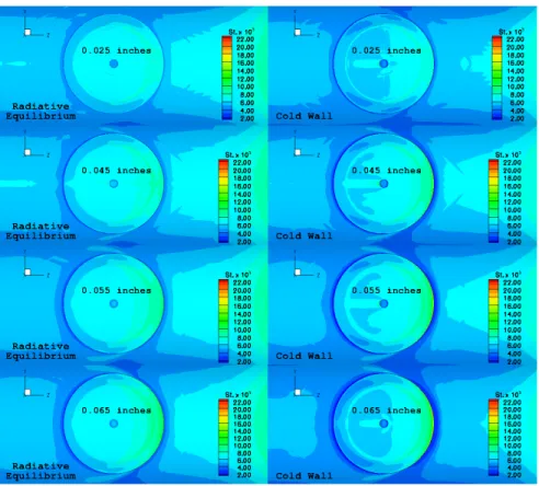
Figure 4. Computed surface heat flux variations on the plug area of the wind tunnel geometries. Flow direction is from right to left.
Contour plots of the computed surface heat fluxes are shown in Figure 4. This figure shows that the plug surface heat flux increases with the plug height. The local surface heat flux is employed and local surface Stanton number is calculated. The main goal of this study is to obtain a correla-tion that may be used for flight condicorrela-tions in which the surface is at radiative equilibrium with surface emissivity of = 0.89. Consequently, the Stanton number is obtained for radiative equilibrium surface conditions. The Stanton number is calculated as
St =qw/(ρ∞V∞Cp(rrfTt−Tw)) (1)
where qw is surface heat flux,ρ∞ is free-stream density, V∞ is free-stream velocity, Cp is specific
heat at constant pressure, rrf is a constant
recov-ery factor,Ttis total temperature, andTwis surface
temperature. The values of free-stream density and velocity are given in Table 1, while values of spe-cific heat, total temperature and wall temperature are given in Table2. A constant recovery factor of 0.92 is used for all the calculations.13 The Surface Stanton number variations are plotted in Figure5.
Specific heat values are calculated based on wind tunnel conditions. For the radiative equilibrium wall condition, local surface temperature is used. Fig-ure 5 shows that the local Stanton number com-puted with the radiative equilibrium wall tempera-ture boundary condition does not entirely match the
one computed with the cold wall boundary condition. The difference is largest at the plug leading edge, and becomes comparable far upstream and downstream of the plug.
Table 2. Parameters used in the Stanton number cal-culations. kp Cp Tw Tt inches BT U/slugs·R R R 0.025 7.7247 526 3110 0.045 7.7081 526 3170 0.055 7.7286 521 3090 0.065 7.7519 525 3020
For all WT cases, the flow spreads to both sides of the plug before passing the plug leading edge and causing a small recirculation region upstream of the plug. Streamlines on the plug top surface are sim-ilar with a recirculation zone just downstream of the cavity trailing edge. These flow features are schematically shown in Figure 6for the 0.065 inch plug.
Computational Validation
The CFD analyses are validated by comparing the numerical data with the WT data. The surface heat flux probe locations are shown in Figure 7. Table 3summarizes differences computational and
exper-imental10 surface heat flux data for all gauge locations. The average of absolute percentage errors are also given in the last column. This table shows that the averaged data from the CFD simulation are within 12% of the experimental data except for the probe number 7 where the average difference is about 30%. Probe 7 is located at the base of the plug where it meets the swept cylinder, and a large error is possibly due to modeling limitation in such area. The average difference between computed and reported WT heat transfer data is about 8% and 9.5% with and without considering probe 7, respectively.
The accuracy of the numerical results are emphasized in Figure 8 by showing heat flux variations with distance along a line that connects two probe points of 1 and 16 (see Figure7a.) Wind tunnel data are also
Figure 5. Stanton number variations on the plug area of the wind tunnel geometries. Flow direction is from right to left.
Figure 7. Surface data points.
Table 3. Differences between computed and measured surface heat flux.
Data Point Error <|Error|>
% %
0.025inches 0.045inches 0.055inches 0.065inches
1 -2.7 +3.0 -1.5 -5.2 3.1 2 -6.8 +13.2 +8.53 +4.4 8.2 3 +17.5 -0.6 +12.4 -12.6 10.8 4 +11.5 +5.9 -10.2 -19.3 11.7 5 +16.9 +1.9 +4.3 -12.8 9.0 6 +13.0 +4.7 +13.0 -2.5 8.3 7 -58.6 +21.0 +34.0 +9.2 30.7 8 -11.8 +24.3 -3.7 -1.6 10.3 9 -11.6 +19.2 +5.6 +7.0 10.8 10 -5.4 +18.9 +11.9 +10.9 11.8 11 +3.3 +19.6 +1.9 -6.5 7.8 12 +0.7 +8.4 +12.0 +3.3 6.1 13 -10.2 +2.4 +13.1 +0.2 6.5 14 -13.1 – -3.4 -8.1 8.2 15 +4.8 13.2 +7.3 +0.8 6.5 16 -11.3 +4.9 +0.4 -6.8 5.9 17 -3.6 +6.4 +6.7 +3.8 5.1
shown in this figure with plug geometry variations. A very good agreement with WT data is achieved. This figure shows that the peak heating increases with the plug height.
(a) 0.025inchplug (b) 0.045inchplug
(c) 0.055inchplug (d) 0.065inchplug
Figure 8. Heat flux variations along the Wind Tunnel (WT) geometry.
To compare heat fluxes on the WT model plug with different heights, the surface heat flux of each model is normalized by the local heat flux at probe location 1. This states the heating Bump Factor, BF. The results are plotted in Figure9. The experimental BF data are also shown in this figure. As shown, BF on the plug top surface increases with plug height. To quantify the CFD accuracy, computed heat fluxes at the gauge locations 1-10 (see Figure 7) are plotted with the measured WT data in Figure 10 in which a good agreement is shown. In this figure, the WT errors are the repeatability errors. This figure shows that that the highest surface heat flux on the plug for all the cases occurs at gauge number 8. The difference between the highest computed and measured heat flux is within 5% for all the cases except for the 0.045 inchcase in which it is 20%. As a result of the good comparisons, these data are employed to develop a generalized heating augmentation correlation that simplifies the prediction process. The intent is then to demonstrate the analysis can be formulated to flight conditions and can be used for flight analysis. This is described in the next section.
Figure 9. Heating Bump Factor, BF, along the Wind Tunnel (WT) geometry.
(a) 0.025inchplug (b) 0.045inchplug
(c) 0.055inchplug (d) 0.065inchplug
Heating Augmentation Correlation
Plug
Smooth surface
!
Peak heating
Base of the plug
Figure 11. Schematic illustration for heating augmen-tation calculation (Eq.2.)
The computational results and the WT data are used to develop a heating augmentation (HA) cor-relation for plug repair at flight conditions. This is obtained by calculating the peak heating rate at the lip of the plug,qη, and the heat flux on the smooth
surface without a plug at a location that would represent the base of the plug if it were present, qbase|no plug, (see Figure11); i.e.
HA= qη
qbase|no plug
, (2)
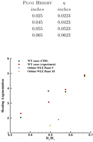
The measured peak heating distance above the surface is shown schematically in Figure11and tab-ulated in Table4 for different plug heights. For the WT models, η is the location of the highest mea-sured gauge.
Table 4. The distance from the base of the plug to a location where the peak heating is measured by gage 8.
Plug Height η inches inches 0.025 0.0223 0.045 0.0423 0.055 0.0523 0.065 0.0623 To obtain heat fluxes at base of the plugs and on
the smooth surface,qbase, simulations are performed
on smooth WT swept cylinder geometries. The peak heating rates are calculated from the gauge 8 loca-tions (see Figure7.) These data are shown in Figure 12 in which the x-axis is the peak heating to free-stream enthalpy ratio, Hη/H∞. Heating augmen-tation on the Space Shuttle Orbiter WLE panels 9 and 18 (see Ref.12) are also computed and shown in this figure. The flight data show that a different correlation parameter is needed to correctly scale WT data (cold wall) to flight data (radiative equi-librium). LAURA is used for all CFD points.
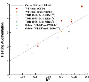
Figure 12. First attempt to scale WT to flight data. An attempt was also made to examine k/δ as
a correlation parameter. This parameter was used by Hung and Patel,11primarily, for largek/δ. They have shown a large uncertainty in heating augmenta-tion associated with this parameter. Our collecaugmenta-tion of data, shown in Figure13, also show thatk/δdoes not correlate well with wide range of conditions.
Examining the enthalpy profile, it was found that the enthalpy profiles of the WT and flight cases start from a different value on the surface due to different wall enthalpy values. Therefore, a correla-tion parameter was chosen that is based on the wall enthalpy values to collapse the WT and the CFD flight data; i.e. Hη/Hw. This correlation parameter
used in Figure14in which the data are presented in log-linear format. Additional CFD flight cases from Ref.4, 5 are also added in this plot. Protuberance to BL thickness ratio, k/δ, for all the presented cases are less than 0.3. It appears that all the presented data points but one are clustered around a single line.
The heating augmentation for the case where Hη/Hw= 1, which is 1, is also shown. This point is
curve-fitted by anchoring the data to the theoretical point, and the following correlation is obtained:
Figure 13. Heating augmentation based onk/δ param-eter, which does not fit the data well.
Figure 14. Proposed heating augmentation parameter for short hypersonic protuberances.
HA= 0.5e0.7Hη/Hw (3)
Applying the Curve-Fita
To use the proposed heating augmentation correla-tion, only a flow field solution over an undisturbed Shuttle geometry is needed. The following steps are then needed to estimate the heating augmentation:
• locate smooth OML geometry that would represent the base of the protuberance if it were presentb
• obtain the wall enthalpy at the identified location, Hw, from the solution
• determine height above the surface that would rep-resent height of the protuberance
• obtain the enthalpy at the identified protuberance lip location,Hη, from the undisturbed flow field
so-lution
• calculate the enthalpy rationHη/Hw
• use the proposed correlation equation, Equation3, to estimate the heating augmentation.
Conclusions
Several CFD analyses are conducted and com-pared with WT results for a swept cylinder model with a protruding rounded plug. It is shown that the CFD data are in very good agreement with mea-sured WT data. Based on the CFD and WT data, a heating augmentation correlation that is based on enthalpy profile is proposed. The proposed equa-tion is examined for several CFD flight cases with short protuberances, where the protuberance to BL thickness ratio is less than 0.3, and a good agreement was achieved. Accordingly, the proposed correlation parameter shows potential for further investigation and testing against more flight cases.
Acknowledgment
The work of the first author is funded by NASA Langley Research Center through contact number NNL06AC49T.
References
1Columbia Accident Investigation Board Final report,
Vols I-IV, URL:htttp://caib.nasa.gov, October, 2003.
aThe curve-fit is only tested for smallk/δ.
2Hung, F., and Patel, D., “Protuberance lnterf erence
Heating in High-speed Flow”, AIAA-84-1724, 1984.
3Lessard, V.R., “CFD-Predicted Tile Heating Bump
Factors Due to Tile Overlay Repairs”, NASA Langley Re-search Center, NASA CR2006-214509, 2006.
4Mazaheri, A.R., “CFD Analysis of Tile-Repair Augers
for the Shuttle Orbiter Re-entry Aeroheating”, NASA Lang-ley Research Center, NASA CR2007-214858, 2007.
5Mazaheri, A.R., “Computational Aerothermodynamic
Analysis of the Space Shuttle Orbiter Tile Overlay Re-pair with Different Geometries”, NASA Johnson Space Cen-ter, Aeroscience and Flight Mechanics Division,EG-SS-07-17, 2007.
6Mazaheri, A.R., and Wood, W.A., “Re-Entry
Aero-heating Analysis of Tile-Repair Augers for the Shuttle Or-biter”, AIAA-2007-4148, 2007.
7White, T., and Tang, C., “CFD Support for CUBRC
RCC Repair”, Aeroheating Panel Review Meeting, Johnson Space Station, Houston, TX, September 2007.
8Gnoffo, P.A., “An Upwind-Biased, Point-Implicit
Re-laxation Algorithm for Viscous, Compressible Perfect-Gas Flows”, NASA TP2953, February 1990.
9Gnoffo, P.A., Gupta, R.N., and Shinn, J.L.,
“Conserva-tion Equa“Conserva-tions and Physical Models for Hypersonic Air Flows in Thermal and Chemical Nonequilibrium”, NASA TP2867, February 1989.
10“Post Test Report for the Aerothermal Wind
Tun-nel Verification Test OH-200 RCC repair C/SiC Plug and NOAX Crack Repair Model Configurations (Model 204-O)”, SE07HB008, The Boeing Company, 2007.
11Hung, F., and Patel, D., “Protuberance INterference
Heating in High-Speed Flow”, AIAA-84-1724.
12Mazaheri, A.R., “Computational Aerothermodynamic
Analysis of Wing Leading Edge Plug Models with Compar-ison to Wind Tunnel Experiments”, NASA Johnson Space Center, Aeroscience and Flight Mechanics Division, EG-SS-07-18, 2007.
13Anderson, B.,Private Communication, NASA Johnson