A Numerical Investigation of Hybrid Flow Control Optimization with Considerations in Optimization

(1)

Washington University in St. Louis

Washington University Open Scholarship

All Theses and Dissertations (ETDs)

January 2010

A Numerical Investigation of Hybrid Flow Control

Optimization with Considerations in Optimization

Matthew Lakebrink

Washington University in St. Louis

Follow this and additional works at:https://openscholarship.wustl.edu/etd

This Thesis is brought to you for free and open access by Washington University Open Scholarship. It has been accepted for inclusion in All Theses and Dissertations (ETDs) by an authorized administrator of Washington University Open Scholarship. For more information, please contact

[email protected].

Recommended Citation

Lakebrink, Matthew, "A Numerical Investigation of Hybrid Flow Control Optimization with Considerations in Optimization" (2010).

All Theses and Dissertations (ETDs). 482.

(2)

WASHINGTON UNIVERSITY IN ST. LOUIS School of Engineering and Applied Science

Department of Mechanical, Aerospace and Structural Engineering

Thesis Examination Committee: Ramesh K. Agarwal, Chair

David A. Peters Kenneth L. Jerina

A NUMERICAL INVESTIGATION OF HYBRID FLOW CONTROL WITH CONSIDERATIONS IN OPTIMIZATION

by

Matthew T. Lakebrink

A thesis presented to the School of Engineering of Washington University in partial fulfillment of the

requirements for the degree of MASTER OF SCIENCE

May 2010 Saint Louis, Missouri

(3)

ii

ABSTRACT OF THE THESIS

A Numerical Investigation of Hybrid Flow Control with Considerations in Optimization

by

Matthew T. Lakebrink

Master of Science in Aerospace Engineering Washington University in St. Louis, 2010 Research Advisor: Professor Ramesh K. Agarwal

The fundamental effects of micro-ramp, synthetic-jet, and hybrid flow control devices are studied through the use of numerical simulations. The beneficial flow control effect is then optimized using the response surface methodology. The effectiveness of each device is judged based on how it influences the shape factor of the boundary layer far downstream of the device. The mechanism of flow control action of each device is a pair of streamwise oriented counter rotating vortices; however, the nature of the vortices produced is unique in each case. The micro-ramp reduced the shape factor by 3.31%, the synthetic-jet by 3.32%, and the hybrid device reduced the shape factor by 3.44% from the baseline. Considering a three factor face-centered central composite design, the hybrid device is optimized capitalizing on the positive effects produced by the micro-ramp and synthetic-jet individually. The device’s performance is shown to be insensitive to the spacing between the micro-ramp and the synthetic-jet. There is, however, a significant sensitivity to the ratio of jet length to jet momentum coefficient. At the optimum value of this ratio (1.33”) the shape factor is decreased by 5.7%.

(4)

iii

Acknowledgments

The first part of this research was supported by the NASA Fundamental Aeronautics Program, Subsonic Fixed Wing Project. I would like to thank Ari Glezer, Abe Gissen, and Bojan Vukasinovic of the Georgia Institute of Technology for their efforts in providing experimental data against which the numerics could be validated. Special thanks to Professor Ramesh Agarwal of Washington University in St. Louis for his patient instruction and guidance throughout this research process.

I would also like to take this opportunity to thank God for blessing me with my talents and desires, my mom for cultivating them, and my wife, to whom this work is dedicated, for her unwavering support and encouragement.

Matthew T. Lakebrink

Washington University in St. Louis May 2010

(5)

iv

List of Figures

Figure 1.1: Development of stall on an airfoil [1]... 2

Figure 1.2:Navier-Stokes DES modeling flow separation in an s-duct diffuser [2] ... 2

Figure 1.3: Mechanism of action for vortex generator flow control [3]... 3

Figure 1.4: Dimensions and Geometry of the Micro-Ramp Vortex Generator... 5

Figure 1.5: Synthetic-Jet Hardware and Dimensions ... 6

Figure 1.6: Top and Side Views of the Geometry and Layout of the Hybrid Flow Control Device... ... 7

Figure 1.7: Three factors with respect to which the hybrid device is locally optimized .... 8

Figure 1.8: Face-centered central composite design for three factors: l, s, and µ... 9

Figure 1.9: Dimensional run matrix for the three factor CCF... 10

Figure 2.1: Computational domain and device placement used for the analysis of the flow control effectiveness... 12

Figure 2.2: Unstructured computational mesh for flow control analysis domain ... 13

Figure 2.3: Increased mesh resolution near the flow control devices and in their wake .. 13

Figure 2.4: Centerline cut through the entire domain (upper) and a close-up of the micro-ramp and structured synthetic-jet block (lower)... 13

Figure 2.5: Geometry for the three cases in the vortex sensitivity analysis ... 14

Figure 2.6: Vortex sensitivity to device placement at a plane far downstream of the throat... 14

Figure 2.7: Computational mesh used for the optimization study... 15

Figure 2.8: Mesh near the flow control devices ... 15

Figure 2.9: Boundary conditions for the flow control analysis domain ... 17

Figure 2.10: Boundary conditions for the hybrid device optimization domain ... 17

Figure 2.11: The time varying behavior of the synthetic-jet is accurately represented by a modified sine wave with an amplitude given by a peak jet velocity which is produced by the response surface based on input frequency and voltage ... 19

(8)

vii

Figure 2.13:Velocity components corresponding to the three coordinate directions...22 Figure 3.1:Boundary layer profile sensitivity to spanwise location at the nearfield in baseline flow ... 24 Figure 3.2:Boundary layer profile sensitivity to spanwise location at the farfield in

baseline flow ... 24 Figure 3.3: Contours of velocity magnitude depicting the boundary layer thickness

at the nearfield and farfield. The vertical lines represent a spanwise

location 2” from the centerline... 25 Figure 3.4: Spanwise shape factor distributions in the nearfield for baseline,

micro-ramp only, synthetic-jet only, and hybrid configurations... 26 Figure 3.5: Spanwise shape factor distributions in the farfield for baseline,

micro-ramp only, synthetic-jet only, and hybrid configurations... 27 Figure 3.6: Iso-surfaces of streamwise vorticity (+/- 10,000/s) and fuselage station

cuttting planes colored by vorticity magnitude ... 28 Figure 3.7: Downstream propagation of the counter-rotating vortex pair induced

by the microramp... 28 Figure 3.8: Full velocity vectors projected onto the nearfield and farfield planes.

Upwash denotes flow away from the wall, while downwash indicates flow toward the wall ... 30 Figure 3.9: Nearfield effects of the microramp on the velocity profiles across the

span ... 30 Figure 3.10: Farfield effects of the microramp on the velocity profiles across the

span... 31 Figure 3.11: Nearfield comparison of baseline and microramp only velocity profiles ... 31 Figure 3.12: Farfield comparison of baseline and microramp only velocity profiles ... 32 Figure 3.13: Behavior of the synthetic-jet throughout its cycle: counter-rotating

streamwise vortex pair formation from blowing portion (top right)

and local downwash from suction portion (bottom right) ... 34 Figure 3.14: Time-averaged solution of synthetic-jet alone with iso-surfaces of

streamwise vorticity at values of +/- 10,000/s ... 34 Figure 3.15: Nearfield effects of synthetic-jet on the velocity profiles across the span.... 35

(9)

viii

Figure 3.16: Farfield effects of synthetic-jet on the velocity profiles across the span ... 36

Figure 3.17: Nearfield comparison of baseline and synthetic-jet only velocity profiles ... 36

Figure 3.18: Farfield comparison of baseline and synthetic-jet only velocity profiles ... 37

Figure 3.19: Vortex core trajectories for the micro-ramp alone (green/upper) and the hybrid (purple/lower) flow control cases... 38

Figure 3.20: Nearfield effects of hybrid actuator on velocity profiles across the span... 39

Figure 3.21: Farfield effects of the hybrid actuator on velocity profiles across the span... 39

Figure 3.22: Farfield comparison of baseline, hybrid, and synthetic-jet... 40

Figure 3.23: Farfield comparison of the hybrid, and synthetic-jet only velocity profiles... 40

Figure 3.24: View looking downstream of the cone of influence resulting from the unsteady synthetic-jet control element: effect with micro-ramp alone (left), synthetic-jet alone (middle), and hybrid device (right)... 41

Figure 3.25: Farfield shape factor distribution across the entire span... 42

Figure 3.26: Shape factor as a function of spanwise averaging width ... 43

Figure 4.1: Shape factors resulting from each of the 15 runs ... 45

Figure 4.2: Vortices and flowfield resulting from DOE configuration one ... 46

Figure 4.3 Vortices and flowfield resulting from DOE configuration two... 47

Figure 4.4: Vortices and flowfield resulting from DOE configuration three... 48

Figure 4.5: Vortices and flowfield resulting from DOE configuration four ... 48

Figure 4.6: Vortices and flowfield resulting from DOE configuration five ... 50

Figure 4.7: Vortices and flowfield resulting from DOE configuration six... 51

Figure 4.8: Vortices and flowfield resulting from DOE configuration seven... 52

Figure 4.9: Vortices and flowfield resulting from DOE configuration eight... 52

Figure 4.10: Vortices and flowfield resulting from DOE configuration nine... 53

Figure 4.11: Vortices and flowfield resulting from DOE configuration ten... 54

Figure 4.12: Vortices and flowfield resulting from DOE configuration eleven ... 55

Figure 4.13: Vortices and flowfield resulting from DOE configuration twelve ... 56

Figure 4.14: Vortices and flowfield resulting from DOE configuration thirteen... 57

(10)

ix

Figure 4.16: Vortices and flowfield resulting from DOE configuration fifteen ... 58

Figure 4.17: Contours of vorticity magnitude at the farfield for configuration seven ... 59

Figure 4.18: Velocity vectors colored by vorticity magnitude at the farfield location for configuration seven (see Figure 4.18 for legend) ... 60

Figure 4.19: Contours of vorticity magnitude at the farfield for configuration two. ... 61

Figure 4.20: Velocity vectors colored by vorticity magnitude at the farfield location for configuration two (see Figure 4.19 for legend)... 61

Figure 4.21: Sensitivity to µ and L at S=1 ... 64

Figure 4.22: Sensitivity to µ and L at S=0.665 ... 64

Figure 4.23: Sensitivity to µ and L at S=0.33 ... 65

Figure 4.24: Sensitivity to µ and S at L=1 ... 65

Figure 4.25: Sensitivity to µ and S at L=0.665 ... 66

Figure 4.26: Sensitivity to µ and S at L=0.33 ... 66

Figure 4.27: Sensitivity to S and L at µ=0.5 ... 67

Figure 4.30: P-values for all factors and interactions ... 69

Figure 4.31: Reduced model sensitivity of h to µ and L... 69

Figure 4.32: Optimum design from the full model ... 70

(11)

x

List of Abbreviations

CFD Computational Fluid Dynamics

RSM Response Surface Methodology

BCFD Boeing Computational Fluid Dynamics

MADCAP Modular Aerodynamic Design Computational Analysis Process

CCF Face Centered Central Composite

CCD Central Composite Design

DOE Design of Experiments

DES Detached Eddy Simulation

RANS Reynolds Averaged Navier-Stokes

URANS Unsteady Reynolds Averaged Navier-Stokes

LES Large Eddy Simulation

NLP Non-Linear Programming

SA Spallart-Allmaras

SST Shear Stress Transport

HLLE Harten-Lax-van Leer-Einfeldt

(12)

1

Chapter 1 Introduction

1.1 Motivation and Goals

Performance, especially efficiency, has long been a key area of competition in the arena of aero vehicle design. Nearly every aircraft in production today has fuel efficiency as one of its top design criteria. With the cost of fuel at an all time high, the demand for ultra efficient aero vehicles has made this constraint more important than ever. Several opportunities exist for efficiency improvements in aero vehicle design, and each one can be viewed as a highly complex problem in optimization.

The present study focuses on the aerodynamic facet of efficiency. Aerodynamic efficiency is important for many parts of the aircraft, especially those subject to an aggressive adverse pressure gradient. For example, flow over a wing will begin to separate and eventually stall at increasingly large angles of attack (Figure 1.1). The stall is accompanied by an abrupt decrease in lift and increase in drag, both of which serve to decrease the efficiency of the aircraft as a whole. Improved airfoil and wing design is one way to push stall to higher angles of attack, or make its effects less abrupt. Unfortunately, a complete redesign of a major aircraft component, like the wing, is not an option for aircrafts already in service. The use of flow control is ideal for situations like this. Adding some form of flow control to the existing wing can provide the needed stall mitigation.

(13)

2

Figure 1.1 Development of stall on an airfoil [1]

Another area where efficiency is greatly affected by strong adverse pressure gradients is in propulsion systems. Flow separation (caused either by an adverse pressure gradient or aggressive geometric design) is one of the major causes of flow quality degradation in propulsion systems, and can result in large pressure recovery loss and decreased system efficiency. Figure 1.2 exemplifies a situation in which a DES captures separation in a highly offset s-duct diffuser. Flow control could be used in this duct to delay separation (or prevent it altogether), and thus decrease the magnitude of losses.

(14)

3

In both cases, and many others, aircraft efficiency is compromised because of the presence or onset of flow separation. One of the best ways to counter the adverse effects of separation is to make sure that the flow never separates to begin with. This is oftentimes achieved through the use of flow control devices. Flow control devices can be active, meaning the device provides some kind of forcing excitation, or it can be passive, meaning the device works just by the flow passing over it. They can be as simple as a rectangular strip of material, or as complicated as an oscillatory plasma actuator. One of the time-tested categories of flow control devices is the vortex generator. Oftentimes the vortex generator is an airfoil section optimized for a certain application, however, a simple plate inclined to the incoming flow is sufficient to produce a vortex. The idea is that the vortex will help the boundary layer ‘recover’ from the effects of an adverse pressure gradient by taking fluid from the high-energy freestream and inserting it into the near-wall region of the boundary layer (Figure 1.3).

Figure 1.3 Mechanism of action for vortex generator flow control [3]

The objective of the present study is two-fold. The first part is to assess a flow control device and to show its effectiveness in terms of potential separation mitigation. This will be done using numerical methods commonly known as computational fluid dynamics (CFD). The device to be investigated is a hybrid vortex generator. It is labeled hybrid because it consists of fluidic and non-fluidic (active and passive) parts.

(15)

4

The fluidic part is a synthetic-jet vortex generator and the non-fluidic part is a micro-ramp vortex generator. Both devices serve to energize the boundary layer through the introduction of high energy flow from the freestream into the near wall region. When used together, a positive additive effect can be realized.

Once the hybrid device is shown to be effective, the second part of the objective for the present study is to determine a local optimum configuration of the hybrid device. This will be done through the use of response surface methodology (RSM) applied to a face centered central composite (CCF) designed experiment.

1.2 Approach to Mitigate Separation

For the present study, a hybrid vortex generator is chosen to mitigate impending separation. The passive part of the hybrid device is a micro-ramp, and the active part is a streamwise oriented slot synthetic-jet. Each component of the hybrid device will be assessed separately and then together in the hybrid formation. The metric by which the flow control will be judged to be either effective or ineffective is the shape factor of the boundary layer on which the device acts. The shape factor is a ratio of the boundary layer’s displacement thickness (Equation 1.1) to its momentum thickness (Equation 1.2) and is given by Equation 1.3.

=

*

δ

∫

∞ ∞ ∞













−

0

1 dy

u

ρ

(Equation 1.1)

∫

∞ ∞ ∞ ∞













−

=

0

1 dy

u

ρ

θ

_{(Equation 1.2)}

θ

δ

*

=

h

_{(Equation 1.3)}

(16)

5

For flows in regions of strong adverse pressure gradients, the shape factor of the boundary layer is large. For this reason, a decrease (over baseline) in boundary layer shape factor will be sought for the flow control devices in order for them to be judged effective.

1.2.1 Passive Flow Control: The Micro-Ramp

The micro-ramp vortex generator gets its name for two reasons. First, the height of the micro-ramp is of the order of one-third the thickness of the boundary layer at the point where it is installed. This height has been shown to be favorable when

compared to larger and smaller ramp heights [4]. If the ramp is too tall, it will act as a significant blockage to the flow, and will produce significant distortion in the downstream boundary layer. On the other hand, if the device is too short, there will not be enough high speed flow to produce effective vortices. The ramp used in this study is shown in Figure 1.4 in planform, side, and isometric views.

0.098” 0.62” 0.56” Flow Dire ction 0.098” 0.62” 0.56” Flow Dire ction

Figure 1.4 Dimensions and Geometry of the Micro-Ramp Vortex Generator

The reason for the second half of this device’s name is apparent from the triangular ramp-like form of the device, depicted in Figure 1.4. Unlike the vortex generator pictured in Figure 1.3, the micro-ramp is considered to be a robust flow control

(17)

6

device. This is because, in application, the micro-ramp device is much less susceptible to breakage or being ‘snapped off’ during maintenance, than its thin plate-like cousin.

1.2.2 Active Flow Control: The Synthetic-Jet

The synthetic-jet gets its name because unlike the traditional jet which, on the time-average, introduces mass into the flow, the synthetic-jet possesses the property of zero net mass flux. This is achieved through the regular oscillatory vibration of two diaphragm membranes. These membranes are the black circular discs shown in Figure 1.5. As the membranes draw away from one another, fluid is pulled in

through the long slot orifice. On the efflux stroke, the membranes push towards each other and force the fluid out of the orifice.

Figure 1.5 Synthetic-Jet Hardware and Dimensions

In this manner, the device is able to potentially impact the flow field without requiring an auxiliary supply of fluid. This is in contrast to traditional jets which oftentimes bleed engine air in order to operate. This results in decreased potential thrust, which is an undesirable side-effect of the traditional jet.

Jet Orifice (1.0 x 0.02) in

(18)

7

1.2.3 Hybrid Flow Control

For the present study, the hybrid device will be formed by placing the synthetic-jet 0.25” upstream of the ramp on its centerline (Figure 1.6).

0.98” 0.02” 0_.5 6 ”

Flow Direction

0.098” 0.98” 0.98” 0.02” 0_.5 6 ”

Flow Direction

0.098” 0.98”

Figure 1.6 Top and Side Views of the Geometry and Layout of the Hybrid Flow Control Device

This particular hybrid configuration was motivated by the hypothesis that the synthetic-jet will serve to augment the effect of he micro-ramp by placing it just upstream. Another logical configuration for the hybrid device would be to place the synthetic-jet just downstream of the ramp on its centerline.

Hybrid devices consisting of a passive device augmented by an active device are often labeled as fail-safe [4]. This is due to the fact that the system can be designed to operate within all acting constraints with the passive device alone. This allows the active device to produce improved flow control effects without having to rely on its durability for safe system operation. For instance, if the synthetic-jet fails, the micro-ramp will still be producing its favorable effect and the system can continue to operate safely, hence it becomes fail-safe.

(19)

8

1.3 Approach to Hybrid Device Optimization

Assuming the hybrid device is able to produce a positive effect on the boundary layer, the device will not necessarily be performing optimally. The design space for the device optimization is exceptionally large, consisting of factors such as jet momentum coefficient, jet orifice shape, jet orifice orientation relative to the mounting surface, ramp height, ramp length, ramp width, ramp angles, location of jet relative to the micro-ramp (which has several factors in and of itself), etc.

For the present study, a small subset (three) of these factors will be chosen for optimization of the hybrid device. These factors are the jet momentum coefficient, jet length (assuming a rectangular orifice as shown in Figure 1.6), and the distance between the trailing edge of the jet and the leading edge of the micro-ramp. These factors are chosen based on their greater importance in the overall effectiveness of the hybrid device for flow control. Figure 1.7 provides a schematic of how these three factors are defined in the device configuration; l is the jet length, s is the jet to ramp spacing, and µ is the jet momentum coefficient defined by Equation 1.4.

(20)

9 2 2 ∞ ∞

≡

V

_JET JET

ρ

µ

_{(Equation 1.4)}

Having identified the three factors for optimization of the hybrid device, a model for the sensitivity of boundary layer shape factor to the three continuously valued factors needs to be created. The method used to create this model is to design an experiment and generate a response surface model from the resulting data. The locations (factor values) for the designed experiment follow the face centered central composite design scheme. The run layout is shown in Figure 1.8 and the corresponding table of

dimensional run data is shown in Figure 1.9. The limits on the factors used in the simulation matrix are determined from intuition and synthetic-jet equipment limitations.

Figure 1.8 Face-centered central composite design for three factors: l, s, and µ

µ

l

s

(21)

10

Figure 1.9 Dimensional run matrix for the three factor CCF

The values for the fitness function (boundary layer shape factor) at each of these points will be obtained from fifteen CFD simulations. A second order response surface will then be fitted to these resulting function values. This surface will be assessed for quality of fit to the data. Once a sufficient fit is achieved, non-linear programming (NLP) methods will be used to find the optimum (minimum) value of the shape factor and the corresponding factor values.

Run S (in) µ l (in)

1 0.33 0.50 1.00 2 0.33 0.30 1.00 3 1.00 0.50 1.00 4 1.00 0.30 1.00 5 0.67 0.40 1.00 6 0.67 0.30 0.67 7 0.67 0.50 0.67 8 0.33 0.40 0.67 9 1.00 0.40 0.67 10 0.67 0.40 0.67 11 0.67 0.40 0.33 12 1.00 0.50 0.33 13 1.00 0.30 0.33 14 0.33 0.50 0.33 15 0.33 0.30 0.33

(22)

11

Chapter 2 Numerical Analysis of the Flow Control

Devices

This chapter sets the stage for the results presented in Chapters 3 and 5. The tools used to perform the numerical analysis, including the grid generator and flow solver, are introduced. In addition, the boundary conditions are presented along with the computational domain in which the governing equations [6] are numerically solved.

2.1 Grid Generation

The software used to create the computational surface meshes used for the present analysis was MADCAP. This software has been developed at Boeing. The volume grids were created based on the aforementioned surface meshes with the AFLR software written by David Marcum of Mississippi State University.

2.1.1 Computational Domains and Meshes

Two computational domains were used in the present study. The first corresponds to the analysis of the micro-ramp, synthetic-jet, and hybrid flow control devices. This computational domain is a replica of the 5” by 5” wind tunnel test section at the Georgia Institute of Technology. A modification of the original test section was made in an effort to highlight the effects caused by the micro-ramp, synthetic-jet, and hybrid devices. This modification was a converging-diverging wall insert. Its intent was to create a mild adverse pressure gradient, without separation, downstream of the geometric throat. Figure 2.1 shows the computational domain and the location of the flow control devices at the throat of the test section. A hybrid grid topology was

(23)

12

chosen with a structured zone to model the synthetic-jet, and multiple unstructured zones used for the remainder of the computational domain. The necessity of the structured grid for modeling the jet region stems from the numerical stability issues caused by the high frequency of the jet actuation.

Flow Direction

0 > ∂ ∂ x P throat plane converging/diverging wall Shear View Plan View synthetic jet microramp

Flow Direction

0 > ∂ ∂ x P

Flow Direction

0 > ∂ ∂ x P throat plane converging/diverging wall Shear View Plan View synthetic jet microramp

Figure 2.1 Computational domain and device placement used for the analysis of the flow control effectiveness

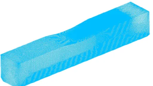
The computational surface mesh for this domain comprised of approximately 260,000 faces is shown in Figure 2.2. A close-up of the surface mesh in the vicinity of the flow control devices is shown in Figure 2.3. The dense packing in the wake of the device is necessary for preserving the flow features produced by the flow control devices as they convect downstream. The red triangular region in both images in Figure 2.3 is the micro-ramp, and the red rectangular region is the portion of the domain modeled with a structured grid. The boundary condition for the synthetic-jet was prescribed on a small subset of the surface within this structured block.

A cut through the centerline of the volume grid is shown in Figure 2.4. The upper image depicts the entire domain, while the lower image is zoomed-in just downstream of the throat in the region where the synthetic-jet and micro-ramp are located. The upper image clearly shows both the prism layer used to resolve the boundary layer (initial spacing at y+=1), and the tetrahedral elements used to capture the general flow through the duct. The lower image in Figure 2.4 shows the structured grid zone used to model the synthetic-jet, and the grid in the vicinity of the micro-ramp.

(24)

13

Figure 2.2 Unstructured computational surface mesh for the flow control analysis domain

Figure 2.3 Increased mesh resolution near the flow control devices and in their wake

Figure 2.4 Centerline cut through the entire domain (upper) and a close-up of the micro-ramp and structured synthetic-jet block (lower)

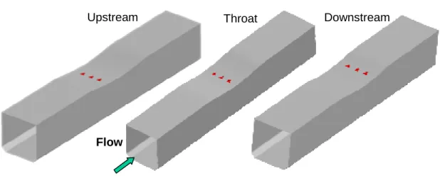
The decision to place the flow control devices just downstream of the throat was the result of a vortex sensitivity study. In this study, three different micro-ramp locations were simulated. The first was just upstream of the throat, the second was directly on the throat, and the third was just downstream of the throat as shown in Figure 2.5. The

(25)

14

strength of the vortices far downstream of the throat was similar for each of the three placements. The real difference was in the location where this strength was

concentrated, as shown by the vorticity contours of Figure 2.6. The upstream

placement resulted in highly distorted vortices, the throat placement resulted in slightly more intact vortices but they occurred significantly away from the wall. The third and most favorable location, just downstream of the throat, realizes the vortices fully intact as well as hugging the wall closely. The ‘well’ of lower vorticity between the wall (red high vorticity region) and the vortex cores (circular regions of vorticity located above the wall) is a region of upwash, and indicates whether the counter rotating vertical structure is preserved. Per the previous observation, these ‘wells’ are not discernable in the upstream placement.

Figure 2.5 Geometry for the three cases in the vortex sensitivity analysis

Figure 2.6 Vortex sensitivity to device placement at a plane far downstream of the throat

Upstream of Throat Throat Downstream of Throat

1000

0

Flow

(26)

15

The second grid was used to conduct the optimization study. The entire grid is shown in Figure 2.7; a close-up of the region where the flow control devices are located is shown in Figure 2.8.

Figure 2.7 Computational mesh used for the optimization study

Figure 2.8 Mesh near the flow control devices

The mesh used in the optimization study consisted of approximately 80,000 surface elements, and 2.25 million volume elements. For two reasons, this mesh was

significantly less complex than the one used to analyze the flow control devices. First, the entire mesh is unstructured where as the first one required a structured block to resolve the synthetic-jet. The reason that the optimization mesh doesn’t require the

(27)

16

structured grid block is described in detail in Section 1 of Chapter 5. The other point of simplification for the optimization mesh is that the flow control devices are located on a flat plate instead of a converging-diverging wall.

2.2 Boundary Conditions

The boundary conditions used in the present study come in two distinct forms. The first set is the conventional set of boundary conditions widely used in numerical simulation of fluid flow. The second set is a strategically created condition used to model the effects a synthetic-jet has on the flow field. These two categories of boundary conditions are described in the following two sections.

2.2.1 Standard Boundary Conditions

The majority of the boundaries in the numerical analysis used in the present study are conventional. Figure 2.9 gives a sketch of the boundary conditions used in the flow control analysis grid. At the entrance (leftmost plane) to the domain, inflow boundary conditions (Mach number, total pressure, total temperature, and flow angularity) are specified. The test section Mach number upstream of the converging-diverging wall is 0.5, the total pressure is14.23 psi, and the total temperature is 537˚R. The total pressure and temperature conditions correspond to the conditions in the wind-tunnel at Georgia Tech. The outflow boundary condition was that of a constant pressure and was approximately 12 psi in order to create the desired flow conditions upstream of the throat. The remainder of the test section, the walls and the micro-ramp, had the no-slip boundary condition applied.

(28)

17

Figure 2.9 Boundary conditions for the flow control analysis domain

Figure 2.10 Boundary conditions for the hybrid device optimization domain Figure 2.10 depicts the boundary conditions used for the optimization domain. The only noteworthy difference from Figure 2.9 is the presence of the symmetry boundary, which was employed to reduce the computational overhead of the optimization effort. On the symmetry boundary, the normal component of velocity is zero.

Inflow Boundary

Freestream Boundary

Outflow Boundary

(29)

18

2.2.2 Synthetic-Jet Boundary Condition

In addition to the aforementioned boundary conditions, in simulations involving a synthetic-jet, the output of the synthetic-jet actuator was modeled as if it was flushed with the surface of the test section wall. The boundary condition was applied to the surface to simulate the jet velocity. It was a modified sine function that was

dependent on the peak jet velocity and the actuator operating frequency (Equation 2.1). The peak jet velocity was computed from a response surface model (RSM) developed by SynGenics Corporation. The actuator RSM was based on a statistical design of experiments (DOE) analysis. This was done to maximize the accuracy of the predicted results while minimizing the number of runs required for model development. The model was a function of the actuator input frequency and voltage (Figure 2.11). The DOE strategy applied to develop the actuator response surfaces was an 11-run, rotatable, central composite design (CCD). This design allows for efficient and accurate estimation of quadratic terms in a regression model.

Furthermore, the use of a rotatable design ensures constant prediction variance at all points equidistant from the design center and thus improves the quality of prediction. The design also includes “replicates” of the center point to quantify experimental error. The response surface analysis of the DOE yielded a modified quadratic equation that accurately predicted the peak synthetic-jet velocity (Upeak) based on voltage and frequency.

( )

ft

U

(30)

19

Figure 2.11 The time varying behavior of the synthetic-jet is accurately represented by a modified sine wave with an amplitude given by a peak jet velocity which is produced by the response

surface based on input frequency and voltage

2.3 The Flow Solver: BCFD

The computational fluid dynamics code used for the present study was BCFD, which has been developed by Boeing. BCFD[10] solves the full Navier-Stokes equation on structured or unstructured grid blocks. Both Spallart-Allmaras [11] and SST turbulence models were used in the present study.

t

U

J

Blowing

Suction

) 2 sin( * ft U UJ = Jpeak π

Vrms

V

=

60 f

=

2 .

2 kHz

Response surface for U

Jpeak

(31)

20

2.3.1 Convergence: Steady State VS. Time-Dependent

Analysis

The baseline solution (empty tunnel with converging-diverging wall only) was achieved by running BCFD in order to solve the steady state governing equations. Convergence was determined by observing the L2 norm and the integrated loads experienced by the walls in the domain. Convergence was considered to be reached when the L2 norm had dropped four or more orders of magnitude, and the loads on the domain had ceased to change from one solver iteration to the next.

The other type of solution obtained in this study was the time-dependent solution for the cases where the flow control devices were present in the tunnel. These solutions were started from the converged steady state solution and then were run by solving the time-dependent governing equations. In each case (micro-ramp alone, synthetic-jet alone, and hybrid) the solution was allowed to iterate in time until the flow had convected one full length of the tunnel, which was approximately 6.3 milliseconds. Beginning at that instant in the time-dependent simulation, a solution was saved every 22.7 microseconds until 100 saves had been made. This gave a simulation which spanned 2.27 milliseconds of physical time, which corresponds to the synthetic-jet undergoing five complete cycles.

2.4 Numerical Data Collection

The data taken from the simulations came from two primary fuselage stations. The first was 2.5” downstream of the throat and the other was 7.5” downstream of the throat (Figure 2.12). The nearfield location was chosen in order to observe the effects of the flow control devices as they were still developing. This was done in an effort to understand not only how the farfield effects were initially formed, but also to gain insight into how the synthetic-jet and micro-ramp combine to form the hybrid effect. The farfield location was chosen to capture the effects of the flow control devices at a

(32)

21

location representative of where an Aerodynamic Interface Plane (AIP) would be located in a practical system.

2.5” (Nearfield) 7.5” (Farfield) throat 5.0” 2.5” (Nearfield) 7.5” (Farfield) throat 5.0”

Figure 2.12 The nearfield and farfield post processing locations

Data that was taken included boundary layer shape factor, time-averaged and jet-phase-locked velocity profiles, time dependent standard deviations in velocity components, vortex core trajectories, and several qualitative sets (meant to capture the flow physics on a more global level). The velocity profiles provided a precise look at what various spanwise locations were experiencing in terms of upwash and downwash. All velocity profiles shown in subsequent chapters have been extracted from the time-averaged solutions, if the simulation dataset was time-dependent. The velocity component definitions used in the results are shown in Figure 2.13.

(33)

22 Z, w X, u Y, v Z, w X, u Y, v

(34)

23

Chapter 3 Resulting Flow Physics

The post processing, which followed analysis of the various flow control devices described in Chapter 1, revealed several interesting results for each device as well as for the baseline flow. This chapter goes into detail on the findings of each of these numerical analyses.

3.1 Baseline

The baseline configuration consisted of flow through the empty tunnel (converging-diverging section only), and provided a reference against which the effectiveness of the flow control devices was measured. The boundary layer profile for the nearfield station is shown in Figure 3.1. The velocity deficit decreases as the spanwise location moves from 2” offset from centerline (CL-2) to the centerline (CL) itself, where the entire tunnel span is 2.5”. The decrease in the deficit is very minimal and overall the boundary layer is of constant thickness 0.25” across the span. This is verified qualitatively in Figure 3.3 where the boundary layer on the upper surface of the left cross section is seen to be uniformly thick between the 2” offset lines. In the corner region, there is an increase in vortical activity in the boundary layer due to the merging of the side and top wall boundary layers, which can be seen from the ‘bulge’ at the corners in Figure 3.3. This vortical activity at the corners manifests itself as an upwash on the flow, which is seen from the slight deficit in the CL-2 curve of Figure 3.1.

(35)

24

Nearfield Baseline Velocity Profiles

0 0.05 0.1 0.15 0.2 0.25 0.3 0.35 0.4 0 0.1 0.2 0.3 0.4 0.5 0.6 0.7 0.8 0.9 1 V/Vinf

Distance From Wall (in)

CL CL-.4 CL-.8 CL-1.2 CL-1.6 CL-2

Figure 3.1 Boundary layer profile sensitivity to spanwise location at the nearfield in baseline flow

Farfield Baseline Velocity Profiles

0 0.1 0.2 0.3 0.4 0.5 0.6 0 0.1 0.2 0.3 0.4 0.5 0.6 0.7 0.8 0.9 1 U/Uinf

CL CL-.4 CL-.8 CL-1.2 CL-1.6 CL-2 V/Vinf

Farfield Baseline Velocity Profiles

0 0.1 0.2 0.3 0.4 0.5 0.6 0 0.1 0.2 0.3 0.4 0.5 0.6 0.7 0.8 0.9 1 U/Uinf

CL CL-.4 CL-.8 CL-1.2 CL-1.6 CL-2 V/Vinf “tick”

Farfield Baseline Velocity Profiles

0 0.1 0.2 0.3 0.4 0.5 0.6 0 0.1 0.2 0.3 0.4 0.5 0.6 0.7 0.8 0.9 1 U/Uinf

CL CL-.4 CL-.8 CL-1.2 CL-1.6 CL-2 V/Vinf

Farfield Baseline Velocity Profiles

0 0.1 0.2 0.3 0.4 0.5 0.6 0 0.1 0.2 0.3 0.4 0.5 0.6 0.7 0.8 0.9 1 U/Uinf

CL CL-.4 CL-.8 CL-1.2 CL-1.6 CL-2 V/Vinf “tick”

(36)

25

Nearfield Farfield

‘bulge’ in boundary layer

V (ft/s) _{V (ft/s)}

Nearfield Farfield

V (ft/s) _{V (ft/s)}

Figure 3.3 Contours of velocity magnitude depicting the boundary layer thickness at the nearfield and farfield. The vertical lines represent a spanwise location 2” from the centerline.

In the farfield, the spanwise variation in boundary layer thickness is more effected by the sidewall boundary layer. This can be seen from the velocity profiles in Figure 3.2 in which the distortion of the profiles is clearly seen at an offset of greater than 1.6” from the centerline. It can be seen in Figure 3.3 that the merging of the boundary layers at the corner has a more far-reaching effect (than in the nearfield) across the span due to the overall thicker boundary layer in this region. As a note, the ‘tick’ present in the CL=1.6 profile of Figure 3.2 shows up in several profiles throughout the results, and is simply an artifact of the grid spacing and not of an actual flow characteristic. At offsets less than 1.6” from the centerline, there is little difference in the boundary layer thickness, which is seen to be about 0.36” (Figure 3.2). The thicker boundary layer in the farfield is due to the dual effect of the lower flow speed (Figure 3.3) and the greater running length to this station.

It is important to notice that at both stations, the effect on the boundary layer profile from the upwash induced by the merging boundary layers decreases from the side wall to the centerline (Figures 3.1 and 3.2). This implies that there is a continuous spanwise distribution of upwash intensity having a minimum at the centerline.

(37)

26

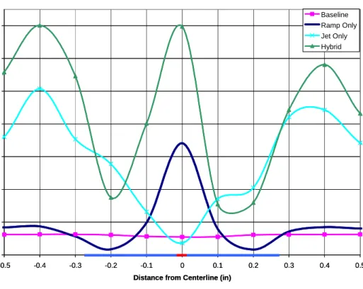
The shape factor within 0.5” of the centerline on either side is basically constant with a value of 1.52 in the near field, and 1.48 in the far field (Figures 3.4 and 3.5). The nearfield boundary layer experiences a much larger adverse streamwise pressure gradient and therefore has a larger shape factor than the farfield location. This indicates that the boundary layer is slightly more prone to separation in the nearfield.

Nearfield Shape Factors

1.4 1.6 1.8 2.0 2.2 2.4 2.6 2.8 -0.5 -0.4 -0.3 -0.2 -0.1 0 0.1 0.2 0.3 0.4 0.5

Distance from Centerline (in) Shape Factor

Baseline Ramp Only Jet Only Hybrid

Microramp width

Jet width

Nearfield Shape Factors

1.4 1.6 1.8 2.0 2.2 2.4 2.6 2.8 -0.5 -0.4 -0.3 -0.2 -0.1 0 0.1 0.2 0.3 0.4 0.5

Microramp width

Jet width

Figure 3.4 Spanwise shape factor distributions in the nearfield for baseline, micro-ramp only, synthetic-jet only, and hybrid configurations

(38)

27

Farfield Shape Factors

1.30 1.35 1.40 1.45 1.50 1.55 1.60 -0.5 -0.4 -0.3 -0.2 -0.1 0 0.1 0.2 0.3 0.4 0.5

Microramp width

Jet width

Farfield Shape Factors

1.30 1.35 1.40 1.45 1.50 1.55 1.60 -0.5 -0.4 -0.3 -0.2 -0.1 0 0.1 0.2 0.3 0.4 0.5

Microramp width

Jet width

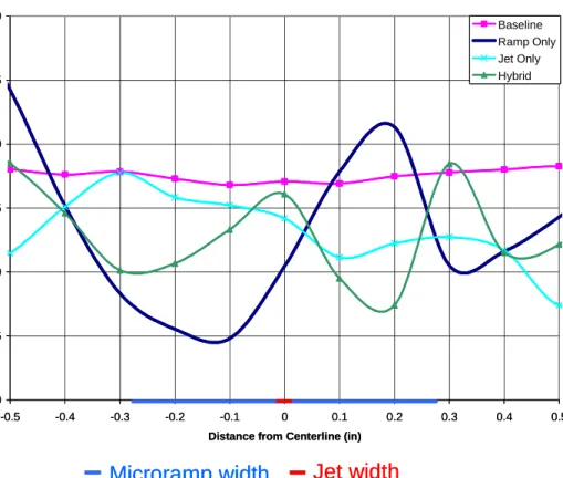
Figure 3.5 Spanwise shape factor distributions in the farfield for baseline, micro-ramp only, synthetic-jet only, and hybrid configurations

3.2 Solitary Micro-Ramp

The addition of the microramp to the flow field had many effects. One very noticeable result was the formation of two counter-rotating streamwise vortices (Figure 3.6). The spanwise spill of flow over the edge of either side of the ramp causes the roll up of this counter-rotating vortex pair, and it convects downstream with the flow (Figure 3.7). It is also clear from Figure 3.7 that as the vortices convect downstream, they lift off the surface slightly. While the sensitivity of boundary layer shape factor to how far the vortex pair is located from the surface is not precisely known, it is intuitive that the closer the vortices remain to the wall the more beneficial their effect will be. This is because as the vortices drift further from the wall, their ability to deposit the high energy freestream flow into the lowest portions of the boundary layer is diminished.

(39)

28

Figure 3.6 Iso-surfaces of streamwise vorticity (+/- 10,000/s) and fuselage station cuttting planes colored by vorticity magnitude.

Farfield

Nearfield

Farfield

Nearfield

Figure 3.7. Downstream propagation of the counter-rotating vortex pair induced by the microramp

A related effect was the establishment of upwash and downwash regions, across the span, of a more intense nature than the corner upwash seen in the baseline flow. In Figure 3.8, the local downwash in the wake of the device is seen to have a larger

(40)

29

magnitude than the ambient downwash, the same is true of the upwash region. The wake is seen to maintain this effect on the boundary layer well downstream to the farfield plane. Figure 3.8 also exemplifies the extent to which the counter rotating vortex structure expands and lifts off the wall as it moves downstream. The main part of the nearfield vortex pair is only about 0.2” wide and hugs the wall very closely whereas in the farfield the vortex pair has grown to be approximately 0.8” wide and has lifted 0.2” off the wall. Velocity profiles across the span support the qualitative findings (Figures 3.9 and 3.10). In the nearfield, the velocity profiles look less full than those from the baseline flow (Figure 3.11). The large deficit at the centerline is due to the strong upwash from the vortex pair produced by the ramp. Moving outboard from the centerline it is observed that the ramp influence diminishes and the velocity profiles regain smoothness, which is indicative of the spanwise extent of the effect the microramp has on the flow (Figure 3.9). At the downstream location, the velocity profiles appear to be much more healthy than in the nearfield. The centerline profile still has a deficit, but it is far less pronounced than in the nearfield profile. The other interesting thing to note is that both the centerline and CL-4 profiles show significant increase in the near-wall velocity when compared to the baseline profiles, and the CL-4 profile is better throughout the boundary layer (Figure 3.12). This effect demonstrates that a microramp alone will energize the lowest portions of the boundary layer far downstream of the device. The profiles regain smoothness outboard of the CL-4 station. This indicates that the outer portion of the vortex is located approximately 0.4” from the centerline, and the total width of effect of the vortex produced by the 0.56” wide microramp is about 0.8” at the farfield location, verifying the qualitative observation from Figure 3.8.

(41)

30

Figure 3.8 Full velocity vectors projected onto the nearfield (left) and farfield (right) planes. Upwash denotes flow away from the wall, while downwash indicates flow toward the wall.

Nearfield Ramp Only Velocity Profiles

0 0.05 0.1 0.15 0.2 0.25 0.3 0.35 0.4 0 0.1 0.2 0.3 0.4 0.5 0.6 0.7 0.8 0.9 1 V/Vinf

CL CL-.4 CL-.8 CL-1.2 CL-1.6 CL-2

Figure 3.9 Nearfield effects of the microramp on the velocity profiles across the span

Nearfield Farfield

Upwash

Downwash Downwash Downwash Upwash Downwash

0.02” 0.1” 0.04” 0.06” Nearfield Farfield Upwash

Downwash Downwash Downwash Upwash Downwash

0.02” 0.1” 0.04” 0.06” 0.4” 0.2” 0.6” 1.0”

(42)

31

Farfield Ramp Only Velocity Profiles

0 0.1 0.2 0.3 0.4 0.5 0.6 0 0.1 0.2 0.3 0.4 0.5 0.6 0.7 0.8 0.9 1 V/Vinf Distance From Wall (in)

CL CL-.4 CL-.8 CL-1.2 CL-1.6 CL-2

Figure 3.10 Farfield effects of the microramp on the velocity profiles across the span

Nearfield Velocity Profiles

0 0.05 0.1 0.15 0.2 0.25 0.3 0.35 0.4 0 0.1 0.2 0.3 0.4 0.5 0.6 0.7 0.8 0.9 1 V/Vinf

Ramp Only CL Ramp Only CL-.4 Baseline CL Baseline CL-.4

(43)

32

Farfield Velocity Profiles

0 0.1 0.2 0.3 0.4 0.5 0.6 0 0.1 0.2 0.3 0.4 0.5 0.6 0.7 0.8 0.9 1 V/Vinf

Ramp Only CL Ramp Only CL-.4 Baseline CL Baseline CL-.4

Figure 3.12 Farfield comparison of baseline and microramp only velocity profiles

The shape factor outside the influence of the vortices was unchanged from the baseline. Within the width of influence, a sharp decrease in shape factor was observed on either side of the centerline where the regions of downwash were identified. There was a sudden increase in shape factor at the centerline corresponding to the strong upwash effect between the vortex pair. This spanwise trend was present both near the device and downstream at the farfield plane (Figures 3.4 and 3.5). The average spanwise value of the shape factor for this case was 1.431, which is a decrease (improvement) from the shape factor of 1.48 realized in the baseline simulation.

3.3 Solitary Synthetic-Jet

When observed alone, the synthetic-jet produced impacts on the flow which were similar in nature to those of the micro-ramp. One difference between the two was the unsteady aspect of the influence with the synthetic-jet compared to the steady nature of the micro-ramp actuator. Like the micro-ramp, the synthetic-jet produced a pair of

(44)

33

counter-rotating streamwise vortices. However, the vortex pair was only generated during the efflux portion of the jet’s cycle (Figure 3.13). While the jet produced suction, the vortices generated during the efflux were allowed to separate from the jet slot and propagate downstream. A time averaged solution shows that regardless of the synthetic-jet having zero net mass flux, the overall effect is the production of two counter-rotating streamwise vortices (Figure 3.14). The farfield is affected by these pulsed vortices and sees a resulting lower average shape factor when compared to the baseline results (Figure 3.5). In fact, the average spanwise shape factor was 1.432. This is an improvement over the baseline flow, and very similar to the shape factor produced by the micro-ramp alone (1.431). The other significant difference between the synthetic-jet and micro-ramp is the spreading effect realized by the vortices as they propagate downstream when they are produced by the synthetic-jet. In the case of the micro-ramp, it was seen that there were two vortices being steadily generated and affecting a downstream region not much wider than the micro-ramp itself. The unsteady nature of the synthetic-jet causes a spanwise destabilization of the boundary layer, resulting in the width of influence spreading to several times the width of the device as the vortices propagate downstream. This increase in the width of influence appears approximately linear with downstream propagation on either side of the centerline, forming a ‘cone’ of influence.

(45)

34 U_jet t Efflux Suction Pair of counter-rotating streamwise vortices are formed

Vortex pair is allowed to separate from jet

and propagate downstream E ffl u x S u ct io n U_jet t Efflux Suction Pair of counter-rotating streamwise vortices are formed

and propagate downstream U_jet t Efflux Suction Pair of counter-rotating streamwise vortices are formed

and propagate downstream E ffl u x S u ct io n

Figure 3.13 Behavior of the synthetic-jet throughout its cycle: counter-rotating streamwise vortex pair formation from blowing portion (top right) and local downwash from suction portion

(bottom right).

F

lo

w

D

ir

e

ct

io

n

Synthetic-Jet (.02” Wide, .98” Long) Counter-Rotating Streamwise Vortices

Co

ne o

f In

_flu

enc

_e

F

lo

w

D

ir

e

ct

io

n

Synthetic-Jet (.02” Wide, .98” Long) Counter-Rotating Streamwise Vortices

Co

ne o

f In

_flu

enc

_e

Figure 3.14 Time-averaged solution of synthetic-jet alone with iso-surfaces of streamwise vorticity at values of +/- 10,000/s.

It is clear from looking at the nearfield velocity profiles (Figure 3.15) that the beneficial effects of the vortices produced by the synthetic-jet do not manifest themselves close to the device. In fact, compared to the baseline profiles in the nearfield, the profiles produced by the synthetic-jet appear to be slightly more prone to separation, especially

(46)

35

at the CL-4 station (Figure 3.17). Far downstream, however, the boundary layer once again shows favorable response to the flow control (Figure 3.16). The profiles at the centerline, CL-4, and CL-8 stations are fuller near the wall than those from the baseline simulation (Figure 3.18), while outboard of the CL-8 station the profiles appear to possess a small increase in velocity deficit. This benefit within 0.8” of the centerline on either side of the 0.02” width synthetic-jet is a more broad favorable influence than that produced by the micro-ramp. This leads to the idea that if both the synthetic-jet and micro-ramp produce beneficial results within the same region on their own, then combining them might produce an even stronger downwash over a potentially wider region. This is the motivation for the hybrid device.

Nearfield Jet Only Velocity Profile

0 0.05 0.1 0.15 0.2 0.25 0.3 0.35 0.4 0 0.1 0.2 0.3 0.4 0.5 0.6 0.7 0.8 0.9 1 V/Vinf

CL CL-.4 CL-.8 CL-1.2 CL-1.6 CL-2

(47)

36

Farfield Jet Only Velocity Profile

0 0.1 0.2 0.3 0.4 0.5 0.6 0 0.1 0.2 0.3 0.4 0.5 0.6 0.7 0.8 0.9 1 V/Vinf

CL CL-.4 CL-.8 CL-1.2 CL-1.6 CL-2

Figure 3.16 Farfield effects of the synthetic-jet on the velocity profiles across the span

Nearfield Velocity Profiles

0 0.05 0.1 0.15 0.2 0.25 0.3 0.35 0.4 0 0.1 0.2 0.3 0.4 0.5 0.6 0.7 0.8 0.9 1 V/Vinf

Jet Only CL Jet Only CL-.4 Baseline CL Baseline CL-.4

(48)

37

Farfield Velocity Profiles

0 0.1 0.2 0.3 0.4 0.5 0.6 0 0.1 0.2 0.3 0.4 0.5 0.6 0.7 0.8 0.9 1 V/Vinf

Jet Only CL Jet Only CL-.4 Jet Only CL-.8 Baseline CL Baseline CL-.4 Baseline CL-.8

Figure 3.18 Farfield comparison of baseline and synthetic-jet only velocity profiles

3.4 Hybrid Device

The combination of the synthetic-jet and micro-ramp in the hybrid flow control device resulted in a favorably augmented control effect. The vortex pair produced by the synthetic-jet was observed to propagate along the micro-ramp and combine with the vortex pair produced by the micro-ramp. Upon interaction of the two pairs of vortices, a distinct augmentation of the size of the combined vortex pair was observed, along with a sharp but brief increase in the magnitude of the vorticity in the vicinity of the device.

A result of the vortices from the synthetic-jet traversing along the micro-ramp is that they are relocated to a distance farther off the wall than when they had the opportunity to propagate downstream without interaction with the micro-ramp. This places the synthetic-jet vortices on top of the vortices produced by the micro-ramp, and effectively ‘holds’ the micro-ramp vortices close to the wall. Indeed, the vortex core trajectories

(49)

38

hug the wall more closely than when there is no synthetic-jet present (Figure 3.19). As the newly formed vortex pair propagates downstream, the augmented size works in combination with the close-to-wall proximity to pull high-energy freestream fluid into the lowest portion of the boundary layer. This is the mechanism by which the hybrid device is able to produce superior changes in the shape factor at the farfield location (Figure 3.5). Averaging the shape factor across the span for this case shows that it has been reduced to 1.429. Again, this is much lower than the baseline, and slightly lower than either the micro-ramp or the synthetic-jet were able to produce independently.

WALL

Flow Direction

Ramp Only Vortex Core Trajectory

Microramp

Hybrid Vortex Core Trajectory WALL

Flow Direction

Ramp Only Vortex Core Trajectory

Microramp

Hybrid Vortex Core Trajectory

Figure 3.19 Vortex core trajectories for the micro-ramp alone (green/upper) and the hybrid (purple/lower) flow control cases

The nearfield velocity profiles for the hybrid configuration (Figure 3.20) display a strong deficit at the centerline and CL-4 stations, indicating that the upwash induced by the hybrid device is dominant in this region. Further downstream (Figure 3.21), the velocity profiles take on a shape more similar to the profiles from the synthetic-jet simulation. At this station, the boundary layer is fuller off the centerline than it is for the baseline and synthetic-jet alone cases (Figure 3.22), and has healthier profiles outboard of the CL-4 station than the synthetic-jet alone (Figure 3.23).

(50)

39

Nearfield Velocity Profile from Hybrid Device

0 0.05 0.1 0.15 0.2 0.25 0.3 0.35 0.4 0 0.1 0.2 0.3 0.4 0.5 0.6 0.7 0.8 0.9 1 V/Vinf

Distance From Wall (in)

CL CL-.4 CL-.8 CL-1.2 CL-1.6 CL-2

Figure 3.20 Nearfield effects of the hybrid actuator on the velocity profiles across the span

Farfield Velocity Profile from Hybrid Device

0 0.1 0.2 0.3 0.4 0.5 0.6 0 0.1 0.2 0.3 0.4 0.5 0.6 0.7 0.8 0.9 1 V/Vinf

Distance From Wall (in)

CL CL-.4 CL-.8 CL-1.2 CL-1.6 CL-2

(51)

40

Farfield Velocity Profiles

0 0.1 0.2 0.3 0.4 0.5 0.6 0 0.1 0.2 0.3 0.4 0.5 0.6 0.7 0.8 0.9 1 V/Vinf

Hybrid CL-.4 Jet Only CL-.4 Baseline CL-.4

Figure 3.22 Farfield comparison of baseline, hybrid, and synthetic-jet only velocity profiles

Farfield Velocity Profiles

0 0.1 0.2 0.3 0.4 0.5 0.6 0 0.1 0.2 0.3 0.4 0.5 0.6 0.7 0.8 0.9 1 V/Vinf Distance From Wall (in)

Hybrid CL-1.6 Jet Only CL-1.6

(52)

41

A view looking downstream of the vorticity field from the micro-ramp to the farfield revealed another interesting finding. The synthetic-jet element again induced spanwise spreading of the width of influence (Figure 3.24). Rather than completely stifling the effect of the synthetic-jet, the micro-ramp only slightly reduces the spanwise destabilization. In addition, the micro-ramp produces larger scale vortices than the jet, which allow for better access to the freestream energy. Indeed, the hybrid effect demonstrated the beneficial spreading effect of the synthetic-jet in conjunction with the powerful large-scale steady vortices produced by the micro-ramp. When compared with the aforementioned configurations, the hybrid device produces the lowest average shape factor at the downstream location.

Microramp alone Jet alone Hybrid

Jet Microramp Jet

Microramp

4.2” 4.2” 4.2”

Microramp alone Jet alone Hybrid

Jet Microramp Jet

Microramp

4.2” 4.2” 4.2”

Figure 3.24 View looking downstream of the cone of influence resulting from the unsteady synthetic-jet control element: effect with micro-ramp alone (left), synthetic-jet alone (middle),

and hybrid device (right).

3.5 A Note on Practical Application

All of the shape factor results reported and displayed so far have been the result of averaging of the spanwise shape factor distribution over 0.5” on either side of the centerline. The motivation for this is due to the fact that this is the region in which the flow control devices appear to produce a favorable change in the near wall velocity. Figure 3.25 shows the shape factor distribution across the entire span, and the corresponding average values of shape factor.

It is clear that averaging over the entire span significantly degrades the performance of the devices in terms of a decrease in shape factor. This emphasizes the point that these devices must be used strategically in a spatial sense, or a large portion of the flowfield

(53)

42

may suffer adverse effects. Figure 3.26 shows the average value of shape factor as a function of the averaging width used. From this figure, it can be seen that each device has an optimal spacing. For instance, the micro-ramp and hybrid devices both show a width of favorable influence of approximately 1.5”, while the synthetic-jet shows a width of favorable influence of about 2.1”. Alternatively, instead of choosing the spacing to achieve an arbitrarily small decrease over baseline shape factor, one could choose to concentrate the devices more heavily to achieve a greater decrease in shape factor across the flow region under consideration. This would be like choosing a micro-ramp spacing of about 0.6”, a synthetic-jet spacing of 1.4”, and a hybrid device spacing of 0.4”. This type of plot can be useful to determine the optimal device spacing when the intent is to use them in an array to control a wide flow region, as would be the case in most practical applications. Making use of this information along with data depicting sensitivity of shape factor to streamwise placement of the devices, one can hone in on the most effective location and array configuration for a given device, thus optimizing a given device in terms of spanwise placement.

Farfield Shape Factors

1.30 1.40 1.50 1.60 1.70 1.80 1.90 2.00 -2.5 -2 -1.5 -1 -0.5 0 0.5 1 1.5 2 2.5

Distance from Centerline (in) H

Baseline Baseline Avg Ramp Only Ramp Only Avg Jet Only Jet Only Avg Hybrid Hybrid Avg

(54)

43

Spanwise Average Shape Factor Distribution 7.5"

Downstream of Throat

1.40 1.45 1.50 1.55 1.60 1.65 1.70 0 0.5 1 1.5 2 2.5 3 3.5 4 4.5 5

Averaging Width About Centerline (in) Average H

(55)

44

Chapter 4 Optimization of the Hybrid Device

4.1 Low Order Synthetic-Jet Modeling

Computational modeling and simulation of the time varying behavior of a synthetic-jet is a time consuming and resource intensive process. This is because instead of getting the steady state governing equations to converge to a single state, the time dependent equations must be converged sufficiently at each instant in time. For these reasons, it is not trivial or even feasible to perform the runs necessary to fill out a design of

experiments matrix while modeling the full unsteady nature of the synthetic-jet. Fortunately, a steady jet can have nearly the same effects as a synthetic-jet with the exception that there is no longer zero net mass flux, which for the purpose of this study is not a significant difference. For the runs performed in this study’s DOE, the effects of the synthetic-jet were achieved by modeling it as a steady jet. This allowed for the steady state governing equations to be solved, significantly decreasing the requirement for computational time.

4.2 Face Centered Central Composite Design

In order to optimize the hybrid flow control device, a model for the sensitivity of boundary layer shape factor to the design variables needed to be created. As mentioned in Chapter 1, the three design factors are the length of the jet, l, the synthetic-jet’s momentum coefficient, µ, and the distance between the leading edge of the micro-ramp and the trailing edge of the synthetic-jet, S. The method used to create this model was to design an experiment and generate a response surface model from the resulting data. The locations (factor values) for the designed experiment follow the face centered central composite design scheme. The run layout is shown in Figure 1.8 and

A Numerical Investigation of Hybrid Flow Control Optimization with Considerations in Optimization

Washington University in St. Louis

Washington University Open Scholarship

A Numerical Investigation of Hybrid Flow Control

Optimization with Considerations in Optimization

Matthew Lakebrink

Acknowledgments

Matthew T. Lakebrink

Contents

List of Figures

List of Abbreviations

Chapter 1

Introduction

1.1

Motivation and Goals

1.2

Approach to Mitigate Separation

=

δ

∫













−

1

dy

u

u

ρ

ρ

∫













−

=

1

dy

u

u

u

u

ρ

ρ

θ

θ

δ

=

h

1.2.1

Passive Flow Control: The Micro-Ramp

1.2.2

Active Flow Control: The Synthetic-Jet

Jet Orifice (1.0 x 0.02) in

1.2.3

Hybrid Flow Control

Flow Direction

Flow Direction

1.3

Approach to Hybrid Device Optimization

≡

V

V

ρ

ρ

µ

µ

l

s

Chapter 2

Numerical Analysis of the Flow Control

Devices

2.1

Grid Generation